Compact and Side Channel Resistant Discrete
Gaussian Sampling
Sujoy Sinha Roy, Oscar Reparaz, Frederik Vercauteren, and Ingrid Verbauwhede
Abstract—Discrete Gaussian sampling is an integral part of
many lattice based cryptosystems such as public-key encryption, digital signature schemes and homomorphic encryption schemes. In this paper we propose a compact and fast Knuth-Yao sampler for sampling from a narrow discrete Gaussian distribution with very high precision. The designed samplers have a maximum sta-tistical distance of2−90 to a true discrete Gaussian distribution.
In this paper we investigate various optimization techniques to achieve minimum area and cycle requirement. For the standard deviation 3.33, the most area-optimal implementation of the bit-scan operation based Knuth-Yao sampler consumes 30 slices on the Xilinx Virtex 5 FPGAs, and requires on average 17 cycles to generate a sample. We improve the speed of the sampler by using a precomputed table that directly maps the initial random bits into samples with very high probability. The fast sampler consumes 35 slices and spends on average 2.5 cycles to generate a sample. However the sampler architectures are not secure against timing and power analysis based attacks. In this paper we propose a random shuffle method to protect the Gaussian distributed polynomial against such attacks. The side channel attack resistant sampler architecture consumes 52 slices and spends on average 420 cycles to generate a polynomial of 256 coefficients.
Keywords. Lattice-based cryptography, Discrete Gaussian Sam-pler, Hardware implementation, Knuth-Yao algorithm, Discrete distribution generating (DDG) tree, Side channel analysis
I. INTRODUCTION
Most currently used public-key cryptosystems are based on difficult number theoretic problems such as integer factoriza-tion or discrete logarithm problem. Though these problems are difficult to solve using present day digital computers, they can be solved in polynomial time on large quantum computers using Shor’s algorithm. Although quantum computing is still in a primitive stage, significant research is going on to develop powerful quantum computers for military applications such as cryptanalysis [1]. As a result, the possible appearance of powerful quantum computers could bring disaster for our present day public-key infrastructure.
Lattice-based cryptography is considered as a strong candi-date for public key cryptography in the era of quantum com-puting. Advantages of lattice-based cryptography over other conventional public key schemes are its strong security proofs,
The authors are with the ESAT/COSIC and iMinds, KU Leuven, Kasteelpark Arenberg 10, B-3001 Leuven-Heverlee, Belgium. Email:
{firstname.lastname}@esat.kuleuven.be This work was supported in part by the Research Council KU Leuven: TENSE (GOA/11/007), by iMinds, by the Flemish Government, FWO G.0213.11N, by the Hercules Foundation AKUL/11/19, by the European Commission through the ICT programme under contract FP7-ICT-2011-284833 PUFFIN and FP7-ICT-2013-10-SEP-210076296 PRACTICE. Sujoy Sinha Roy is funded by an Erasmus Mundus fellowship.
vast range of applicability [2] and computational efficiency. In the present decade, beside significant progress in the theory of lattice-based cryptography, efficient implementations [3], [4], [5], [6], [7], [8], [9], [10], [11], [12], [13] have increased practicality of the schemes.
Sampling from a discrete Gaussian distribution is an essen-tial part in many lattice-based cryptosystems such as public key encryption, digital signature and homomorphic encryption. Hence an efficient and secure implementation of discrete Gaussian sampling is a key towards achieving practical im-plementations of these cryptosystems. To achieve efficiency, the sampler architecture should be small and fast. At the same time the sampler should be very accurate so that its statistical distance to a true discrete Gaussian distribution is negligible to satisfy the security proofs [14].
The most commonly used methods for sampling from a discrete Gaussian distribution are based on the rejection and inversion methods. However these methods are very slow and consume a large number of random bits. The first hardware implementation of a discrete Gaussian sampler [4] uses a Gaussian distributed array indexed by a (pseudo)random num-ber generator. However the sampler has a low precision and a small tail bound (2s) which results in a large statistical distance to the true discrete Gaussian distribution. A more efficient sampler in [6] uses an inversion method which compares random probabilities with a cumulative distribution table. In the hardware architecture an array of parallel comparators is used to map a random probability into a sample value. To satisfy a negligible statistical distance, the sampler requires very large comparator circuits. This increases area and delay of the sampler. The first compact implementation with negligible statistical distance was proposed in [7]. The sampler is based on the Knuth-Yao random walk algorithm [15]. The advantage of this algorithm is that it requires a near-optimal number of random bits to generate a sample point in the average case. The sampler was designed to attain a statistical distance less than 2−90 to a true discrete distribution for the standard deviation
Our contributions: In this paper we propose a compact and
fast discrete Gaussian sampler based on the Knuth-Yao random walk. As the Knuth-Yao random walk is not a constant-time operation, the discrete Gaussian sampler is vulnerable to side-channel attacks. In this paper we propose a technique to prevent such attacks. In particular, we make the following contributions:
1) The compact Knuth-Yao sampler proposed in [7] is composed of mainly a ROM, a scan register and several small counters. The sampler consumes 47 slices on a Xilinx Virtex 5 FPGA for the standard deviation σ= 3.33. The area requirement of the sampler is mostly due to the ROM and the scan-register. In this paper we reduce the total area consumption of the sampler by reducing the width of the ROM and the scan-register. We also optimize the control signal generation block to finally achieve an area of only 30 slices for the overall sampler. In this paper we provide a detailed internal architecture of the sampler along with the control signal generation block.
2) The basic Knuth-Yao sampler [7] performs a random walk determined by a sequence of random bits and by the probability bits from the ROM. This bit scanning op-eration is sequential and thus the sampler in [7] requires on average 17 cycles to obtain a sample point. To achieve faster computation time, we increase the speed of the sampler by using a dedicated small lookup table that maps the initial random bits directly into a sample point (with large probability) or into an intermediate position in the random walk.
3) The Knuth-Yao random walk is not a constant time operation and hence it is possible by an adversary to predict the value of the output sample by performing timing and simple power analysis. In this paper we show how this side channel analysis can be used to break the ring-LWE encryption scheme. Finally we propose a random shuffle method to remove any timing information from a Gaussian distributed polynomial.
The remainder of the paper is organized as follows: Sec-tion II provides a brief mathematical background. Imple-mentation strategies for the Knuth-Yao sampler architecture are described in Section III. The hardware architecture for the discrete Gaussian sampler is presented in Section IV. In Section V we describe side channel vulnerability of the sampler architecture along with countermeasures. Detailed experimental results are presented in Section VI.
II. BACKGROUND
Here we recall the mathematical background required to understand the paper.
A. Discrete Gaussian Distribution
A discrete Gaussian distribution defined over Z with stan-dard deviation σ >0 and mean c ∈Z is denoted as DZ,σ,c.
LetE be a random variable distributed as perDZ,σ,c. This is
defined as follows.
P r(E=z) = 1 Se
−z2/2σ2
whereS= 1 + 2 ∞ X
z=1
e−z2/2σ2
The normalization factorS is approximatelyσ√2π. For most lattice based cryptosystems the mean c is taken as zero and in such cases we use DZ,σ to represent DZ,σ,0. A discrete
Gaussian distribution can also be defined over a lattice L ⊆
Rm. Such a distribution is denoted as DL,σ and assigns a probability proportional toe−|x|2/2σ2
to each element x∈L. WhenL=Zm, the discrete Gaussian distribution DL,σ over Lis the product distribution ofmindependent copies ofDZ,σ.
B. Tail and precision bounds
A discrete Gaussian distribution has an infinitely long tail and infinitely high precision for the probabilities of the sample points. In a real-world application it is not possible to design a sampler that can support infinite tail and precision. Indeed in practical applications we put an upper bound on the tail and the precision of the probabilities. Such bounds obviously introduce a non-zero statistical distance to a true discrete Gaussian distribution. To satisfy the security proofs [14], the sampler should have a negligible statistical distance to a true discrete Gaussian distribution. According to Lemma 4.4 in [17], for anyc >1the probability of sampling v fromDZm,σ satisfies the following inequality.
P r(|v|> cσ√m)< cmem2(1−c2) (1) Similarly denote the probability of samplingz∈Z accord-ing to the accurate distribution DZ,σ with ρz. Assume that the real-world sampler sampleszwith probabilitypz and the corresponding approximate distribution is D˜Z,σ. There is an error-constant ǫ > 0 such that |pz−ρz| < ǫ. The statistical distance between D˜Zm,σ corresponding to m independent samples fromD˜Z,σ and the true distributionDZm,σ [18]:
∆( ˜DZm,σ, DZm,σ)<2−k+ 2mztǫ . (2)
Here P r(|v| > zt : v ← DZm,σ) < 2−k represents the tail bound.
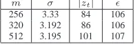
In Table I we show the tail bound |zt| and the precision boundǫ required to satisfy a statistical distance of less than 2−90 for the Gaussian distribution parameter sets taken from [4]. We first calculate the tail bound|zt|from Equation 1 for the right-hand side upper bound2−100. Then using Equation 2,
we derive the precision ǫ for a maximum statistical distance of 2−90 and the value of the tail bound |zt|. In practice
m σ |zt| ǫ
256 3.33 84 106 320 3.192 86 106 512 3.195 101 107
TABLE I
PARAMETER SETS AND PRECISIONS TO ACHIEVE STATISTICAL DISTANCE LESS THAN2−90
0 1 1 1 0
0 0 1 0 1 0 1 1 0 1 Pmat =
I
level 0
I
I
1
0
level 1
I
2
1
0
I
0
I
2
1
row 0
column 0
root
Fig. 1. Probability matrix and corresponding DDG-tree
C. The Knuth-Yao Algorithm
The Knuth-Yao sampling algorithm performs a random walk along a binary tree known as the discrete distribution generat-ing (DDG) tree. A DDG tree is related to the probabilities of the sample points. The binary expansions of the probabilities are written in the form of a binary matrix which we call the
probability matrixPmat. In the probability matrix thejth row corresponds to the probability of thejth sample point.
A DDG tree consists of two types of nodes : intermediate nodes (I) and terminal nodes. A terminal node contains a sample point, whereas an intermediate node generates two child nodes in the next level of the DDG tree. The number of terminal nodes in the ith level of a DDG is equal to the Hamming weight of theith column of the probability matrix. An example of a DDG tree corresponding to a probability distribution consisting of three sample points {0,1,2} with probabilities p0 = 0.01110,p1 = 0.01101andp2= 0.00101
is shown in Figure 1. During a sampling operation a random walk is performed starting from the root of the DDG tree. For every jump from one level of the DDG tree to the next level, a random bit is used to determine a child node. The sampling operation terminates when the random walk hits a terminal node. The value of the terminal node is the value of the output sample point.
A naive implementation of a DDG tree requires O(ztǫ) storage space where the probability matrix has a dimension (zt + 1) ×ǫ. However in practice much smaller space is required as a DDG tree can be constructed on-the-fly from the corresponding probability matrix.
III. EFFICIENTIMPLEMENTATION OF THEKNUTH-YAO ALGORITHM
In this section we present a simple hardware implementation friendly construction of the Knuth-Yao sampling algorithm from our previous paper [7]. However this basic construction is slow due to its sequential bit-scanning operation. In the end of this section we propose a fast sampler architecture using a precomputed lookup table.
A. Construction of the DDG tree at runtime
The Knuth-Yao random walk travels from one level of the DDG tree to the next level after consuming a random bit. During a random walk, the ith level of the DDG tree is constructed from the (i−1)th level using the ith column of the probability matrix. Hence in an efficient implementation of the sampling algorithm, we need to work with only one level of the DDG tree and one column of the probability matrix at a time.
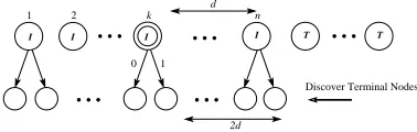
A Knuth-Yao traversal from the(i−1)th level of the DDG tree to theith level is shown in Figure 2. Assume that in the (i−1)th level, the visited node is the kth intermediate node and that there aredintermediate nodes to the right side of the visited node. Now the random walk consumes one random bit and visits a child node in theith level of the DDG tree. The visited node has2dor2d+ 1nodes to its right side depending on whether it is a right or a left child of its parent node. Now to discover the terminal nodes in this level of the DDG tree, the ith column of the probability matrix is scanned from the bottom. Each ‘1’ bit in the column discovers a terminal node from the right side of the ith level of the DDG tree. The value of the terminal node is the corresponding row number for which it was discovered. In this way the visited node will eventually be discovered as a terminal node if the Hamming weight of theith column is larger than the number of nodes present to the right side of the visited node. When the visited node is discovered as a terminal node, the sampling operation stops and the corresponding row number of the probability matrix is the value of the sample. For the other case, the random walk continues to the(i+ 1)th level of the DDG tree and then the same process continues until a terminal node is visited by the random walk.
The traversal can be implemented using a counter which we call distance counter and a register to scan a column of the probability matrix. For each jump to a new level of the DDG tree the counter is initialized to2dor2d+ 1depending on the random bit. Then the corresponding column of the probability matrix is scanned from the bottom using the bit-scan register. Each ‘1’ bit read from the bit-scanning operation decrements the distance counter. The visited node is discovered as a terminal node when the distance counter becomes negative for the first time.
B. Optimized storage of the probability bits
In the last subsection we have seen that during the Knuth-Yao random walk probability bits are read from a column of the probability matrix. For a fixed distribution the probability values can be stored in a cheap memory such as a ROM. The way in which probability bits are stored in the ROM affects the number of ROM accesses and hence also influences the performance of the sampler. Since the probability bits are read from a single column during the runtime construction of a level in the DDG tree, the number of ROM accesses can be minimized if the columns of the probability matrix are stored in the ROM words.
A straightforward storage of the columns would result in a redundant memory consumption as most of the columns in the probability matrix contains a chain of 0s in the bottom. In
T
I T
I I I
1 2 k
d n
Discover Terminal Nodes
2d
1 0
001101001000110011101100011010 001010010010001110000011001110 000111010011001101100110100000 000100101100101100100011010010 000010101111011110010010001110
000000010011011000000110100010 000000000111101001000111111011 000000000010101110111011001001 000000000000111000101110001100
000000000000000001000100110001 000000000000000000001111000100 000000000000000000000010111111 000001011100110110001001011000 000000101100100010110010101101
000000000000010000101011010101 000000000000000100011100100010 001111001101110110011011001101
#0 #2 #1
001110_1110111_110 11011_110010111_11 000111111111010111000101110101
Part of Probability Matrix First two ROM words
Fig. 3. Storing Probability Matrix
an optimized storage these 0s can be compressed. However in such a storage we also need to store the lengths of the columns as the columns will have variable lengths after trimming off the bottom 0s. If the column lengths are stored naively, then it would cost ⌈logztσ⌉ bits per column and hence in total ǫ⌈logztσ⌉ bits. By observing a special property of the Gaussian distributed probability values, we can indeed derive a much simpler and optimized encoding scheme for the column lengths. In the probability matrix we see that for most of the consecutive columns, the difference in the column lengths is either zero or one. Based on this observation we use one-step differential encoding scheme for the column lengths : when we move from one column to its right consecutive column, then column length either increases by one or remains the same. Such a differential encoding scheme requires only one bit per column length. In Figure 3 we show how the bottom zeros are trimmed using one-step partition line. In the ROM we store only the portion of the probability matrix that is above the partition line. Along with the columns, we also store the encoded column-length bit. Each column starts with a column length bit : if this bit is ‘1’, then the column is larger by one bit compared to its left consecutive column; otherwise they are of equal lengths.
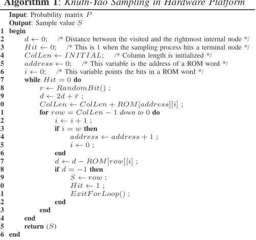
We take Algorithm 1 from [7] to summarize the steps of the Knuth-Yao sampling operation. The ROM has a word size of wbits and contains the probability bits along with the column-length bits.
C. Fast sampling using lookup table
A Gaussian distribution is concentrated around its center. In the case of a discrete Gaussian distribution with standard deviation σ, the probability of sampling a value larger than t·σis less than2 exp(−t2/2) [17]. In fact this upper bound
is not very tight. We use this property of a discrete Gaussian distribution to design a fast sampler architecture satisfying the speed constraints of many real-time applications. As seen from the previous section, the Knuth-Yao random walk uses random bits to move from one level of the DDG tree to the next level. Hence the average case computation time required per sampling operation is determined by the number of random bits required in the average case.
The lower bound on the number of random bits required per sampling operation in the average case is given by the entropy of the probability distribution [19]. The entropy of a
continuous normal distribution with a standard deviationσ is
1
2log(2πeσ
2). For a discrete Gaussian distribution, the entropy
is approximately close to entropy of the normal distribution with the same standard deviation. A more accurate entropy can be computed from the probability values as per the following equation.
H =−
∞ X
−∞
pilogpi (3)
The Knuth-Yao sampling algorithm was developed to consume the minimum number of random bits on average [15]. It was shown that the sampling algorithm requires at most H + 2 random bits per sampling operation in the average case.
For a Gaussian distribution, the entropyH increases with the standard deviation σ, and thus the number of random bits required in the average case also increases with σ. For applications such as the ring-LWE based public key encryption scheme and homomorphic encryption, smallσis used. Hence for such applications the number of random bits required in the average case are small. Based on this observation we can avoid the costly bit-scanning operation using a small precomputed table that directly maps the initial random bits into a sample value (with large probability) or into an intermediate node in the DDG tree (with small probability). During a sampling operation, first a table lookup operation is performed using the initial random bits. If the table lookup operation returns a sample value, then the sampling algorithm terminates. For the other case, bit scanning operation is initiated from the intermediate node. For example, when σ = 3.33, if we use a precomputed table that maps the first eight random bits, then the probability of getting a sample value after the table lookup is 0.973. Hence using the lookup table we can avoid the costly bit-scanning operation with probability 0.973. However extra storage space is required for this lookup table. When the probability distribution is fixed, the lookup table
Algorithm 1: Knuth-Yao Sampling in Hardware Platform
Input: Probability matrixP
Output: Sample valueS
begin 1
d←0; /* Distance between the visited and the rightmost internal node */
2
Hit←0; /* This is 1 when the sampling process hits a terminal node */
3
ColLen←IN IT IAL; /* Column length is initialized */
4
address←0; /* This variable is the address of a ROM word */
5
i←0; /* This variable points the bits in a ROM word */
6
whileHit= 0do
7
r←RandomBit();
8
d←2d+ ¯r;
9
ColLen←ColLen+ROM[address][i];
10
forrow=ColLen−1down to0do 11
i←i+ 1;
12
ifi=wthen
13
address←address+ 1;
14
i←0;
15
end 16
d←d−ROM[row][i];
17
ifd=−1then
18
S←row;
19
Hit←1;
20
ExitF orLoop();
21
end 22
end 23
end 24
return (S)
can be implemented as a ROM which is cheap in terms of area in hardware platforms. In the next section we propose a cost effective implementation of a fast Knuth-Yao sampler architecture.
IV. THESAMPLERARCHITECTURE
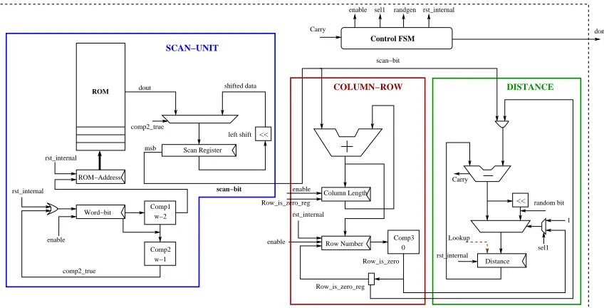
The first hardware implementation of a Knuth-Yao sampler was proposed in our previous paper [7]. In this paper we optimize the previous sampler architecture and also introduce a lookup table that directly maps input random bits into a sample point or into an intermediate node in the DDG tree. The sampler architecture is composed of 1) a bit-scanning unit, 2) counters for column length and row number, and 3) a subtraction-based down counter for the Knuth-Yao distance in the DDG tree. In addition, for the fast sampler architecture, a lookup table is also used. A control unit is used to gen-erate control signals for the different blocks and to maintain synchronization between the blocks. The control unit used in this paper is more decentralized compared to the control unit in [7]. This decentralized control unit has a more simplified control logic which reduces the area requirement compared to the previous architecture. We now describe the different components of the sampler architecture.
A. The Bit-scanning Unit
The bit-scanning unit is composed of a ROM, a scan register, one ROM-address counter, one counter to record the number of bits scanned from a ROM-word and a comparator. The ROM contains the probabilities and is addressed by the ROM-address counter. During a bit-scanning operation, a ROM-word (size w bits) is first fetched and then stored in the scan register. The scan-register is a shift-register and its msb is read as the probability-bit. To count the number of bits scanned from a ROM-word, a counter word-bit is used. When the word-bit counter reachesw−2from zero, the output from the comparator Comp1 enables the ROM-address counter. In the next cycle the ROM-address counter addresses the next ROM-word. Also in this cycle the word-bit counter reaches w−1 and the output from Comp2 enables reloading of the bit-scan register with the new ROM-word. In the next cycle, the word-bit counter is reset to zero and the bit-scan register contains the word addressed by the ROM-word counter. In this way data loading and shifting in the bit-scan register takes place without any loss of cycles. Thus the frequency of the data loading operation (which depends on the widths of the ROM) does influence the cycle requirement of the sampler architecture. This interesting feature of the bit-scan unit will be utilized in the next part of this section to achieve optimal area requirement by adjusting the width of the ROM and the bit-scan register. Another point to note in this architecture is that, most of the control signals are handled locally compared to the centralized control logic in [7]. This effectively simplifies the control logic and helps in reducing area. The bit-scanning unit is the largest sub-block in the sampler architecture in terms of area. Hence this unit should be designed carefully
to achieve minimum area requirement. In FPGAs a ROM can be implemented as a distributed ROM or as a block RAM. When the amount of data is small, a distributed ROM is the ideal choice. The way a ROM is implemented (its width w and depthh) affects the area requirement of the sampler. Let us assume that the total number of probability bits to be stored in the ROM is Dand the size of the FPGA LUTs is k. Then the total number of LUTs required by the ROM is around
⌈wD·2k⌉ ·walong with a small amount of addressing overhead. The scan-register is a shift register of widthwand consumes aroundwLUTs andwf =wFFs. Hence the total area (LUTs and FFs) required by the ROM and the scan-register can be approximated by the following equation.
#Area = D
w·2k
·w+ (w+wf)
= h
2k
·w+ (w+wf)
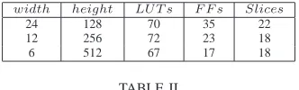
For optimal storage,hshould be a multiple of2k. Choosing a larger value ofhwill reduce the width of the ROM and hence the width of the scan-register. However with the increase in h, the addressing overhead of the ROM will also increase. In Table II we compare area of the bit-scan unit for σ = 3.33 with various widths of the ROM and the scan register using Xilinx Virtex V xcvlx30 FPGA. The optimal implementation is achieved when the width of the ROM is set to six bits. Though the slice count of the bit-scan unit remains the same in both the second and third column of the table due to various optimizations performed by the Xilinx ISE tool, the actual effect on the overall sampler architecture will be evident in Section VI.
B. Row-number and Column-length Counters
As described in the previous section, we use a one-step differential encoding for the column lengths in the probability matrix. The column-length counter in Figure 4 is an up-counter and is used to represent the lengths of the columns. During a random-walk, this counter increments depending on the column-length bit which appears in the starting of a column. If the column-length bit is zero, then the column-length counter remains in its previous value; otherwise it increments by one. At the starting of a column-scanning operation, the
Row-number counter is first initialized to the value of
column-length. During the scanning operation this counter decrements by one in each cycle. A column is completely read when the
Row Number counter reaches zero.
C. The Distance Counter
A subtraction-based counter distance is used to keep the distance d between the visited node and the right-most
width height LUT s F F s Slices
24 128 70 35 22
12 256 72 23 18
6 512 67 17 18
TABLE II
<<
<<
Scan Register dout shifted data
ROM−Address
Word−bit w−2
Comp2 w−1 Comp1 rst_internal
rst_internal
enable
scan−bit
SCAN−UNIT
Row Number Comp30
Row_is_zero_reg enable
Row_is_zero
COLUMN−ROW DISTANCE
scan−bit
ROM
1
sel1
done Carry
enable sel1 randgen rst_internal
Control FSM
msb
left shift
comp2_true
comp2_true
rst_internal Row_is_zero_reg
enable Column Length
rst_internal Distance
random bit Carry
Lookup
Fig. 4. Hardware Architecture for Knuth-Yao Sampler
intermediate node in the DDG tree. The register distance is first initialized to zero. During each column jump, the
row zero reg is set and thus the subtrahend becomes zero.
In this step, the distance register is updated with the value2d or2d+ 1depending on the input random bit. As described in the previous section, a terminal node is visited by the random walk when the distance becomes negative for the first time. This event is detected by the control FSM using the carry generated from the subtraction operation.
After completion of a random walk, the value present in
Row Number is the magnitude of the sample output. One
random bit is used as a sign of the value of the sample output.
D. The Lookup Table for Fast Sampling
The output from the Knuth-Yao sampling algorithm is deter-mined by the probability distribution and by the input sequence of random bits. For a given fixed probability distribution, we can precompute a table that maps all possible random strings of bit-width s into a sample point or into an intermediate distance in the DDG tree. The precomputed table consists of 2s entries for each of the2spossible random numbers.
On FPGAs, this precomputed table is implemented as a distributed ROM using LUTs. The ROM contains 2s words and is addressed by random numbers of s bit width. The success probability of a table lookup operation can be in-creased by increasing the size of the lookup table. For example when σ= 3.33, the probability of success is 0.973 when the lookup table maps the eight random bits; whereas the success probability increases to 0.999 when the lookup table maps 13 random bits. However with a larger mapping, the size of precomputed table increases exponentially from 28 to213.
Additionally each lookup operation requires 13 random bits. A more efficient approach is to perform lookup operations in steps. For example, we use a first lookup table that maps the first eight random bits into a sample point or an intermediate distance (three bit wide for σ = 3.33). In case of a lookup
failure, the next step of the random walk from the obtained intermediate distance will be determined by the next sequence of random bits. Hence, we can extend the lookup operation to speedup the sampling operation. For example, the three-bit wide distance can be combined with another five random bits to address a (the second) lookup table. Using this two small lookup tables, we achieve a success probability of 0.999 for σ = 3.33. An architecture for a two stage lookup table is shown in Figure 5.
V. TIMING ANDSIMPLEPOWERANALYSIS
The Knuth-Yao sampler presented in this paper is not a constant time architecture. Hence this property of the sampler leads to side channel vulnerability. Before we describe this in detail, we first describe the ring-LWE encryption scheme which requires discrete Gaussian sampling from a narrow distribution.
A. The ring-LWE Encryption Scheme
The ring-LWE encryption scheme [20] uses special struc-tured ideal lattices. Such ideal lattices are a generalization of cyclic lattices and correspond to ideals in rings Z[x]/hfi,
wheref is an irreducible polynomial of degree n. To reduce
Sample Sample
Initial Distance Lookup
Table 2 Lookup
Table 1
Random Bits LU1 Distance
computation cost, the underlying ring is generally taken as Rq =Zq[x]/hfi with the irreducible polynomial of the form
f(x) =xn+ 1, wherenis a power of two and the primeqis taken as q≡1 mod 2n. The ring-LWE distribution consists of tuples (a, t) where the polynomial a is chosen uniformly from Rq and t = a·s+e ∈ Rq. The polynomial s is a secret polynomial and is a fixed polynomial for a ring-LWE distribution. The error polynomialeis constructed by sampling its coefficients from a discrete Gaussian distributionXσ. Key generation, encryption and decryption are as follows:
1) KeyGeneration(a): Two polynomialsr1, r2∈Rq are
chosen from Xσ and then p = r1 −a·r2 ∈ Rq is
computed. The public key is the polynomial pair(a, p) and the private key is the polynomialr2.
2) Encryption(a, p, m): The messagem is first encoded to a polynomialm¯ ∈ Rq. Then three error polynomi-als e1, e2, e3 ∈ Rq are constructed by sampling their
coefficients from from a discrete Gaussian distribu-tion with standard deviadistribu-tion σ. The ciphertext is the polynomial pair (c1, c2) where c1 = a·e1+e2 and
c2=p·e1+e3+ ¯m∈Rq.
3) Decryption(c1, c2, r2) : First a polynomial m′ = c1·
r2+c2 ∈ Rq is computed. Then the original message
mis recovered fromm′ using a simple decoder.
B. Side Channel Vulnerability of the Sampling Operation
In the ring-LWE encryption scheme, the key generation and the encryption require discrete Gaussian sampling. The key generation operation is performed only to generate long-term keys and hence can be performed in a secure environment. However, this is not the case for the encryption operation. It should be noted that in a public key encryption scheme, the plaintext is normally considered secret information. For example, it is common practice to use a public-key cryptosys-tem to encrypt a symmetric key that is subsequently used for fast, bulk encryption (this construction is commonly named “hybrid cryptosystems”). Hence, from the perspective of side-channel analysis, any leak of information during the encryption operation about the plaintext (symmetric key) is considered as a valid security threat.
The basic Knuth-Yao sampler uses a bit scanning operation in which the sample generated is related to the number of probability-bits scanned during a sampling operation. Hence, the number of cycles of a sampling operations provides some information to an attacker about the value of the sample. We recall that in a ring-LWE encryption operation, the Gaussian sampler is used as a building block, and it is called in an iterative fashion to generate an array of samples. An attacker that monitors the instantaneous power consumption of the discrete Gaussian sampler architecture can easily retrieve accu-rate timings for each sampling information via Simple Power Analysis (SPA) patterns, and hence gain some information about the secret polynomialse1,e2 ande3. In the worst case,
this provides the adversary with enough information to break the cryptosystem.
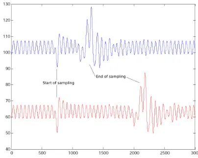
To verify to what extent the instantaneous power consump-tion provides informaconsump-tion about the sampling operaconsump-tion, we
performed a SPA attack on the unprotected design running on a Xilinx Spartan-III at 40 MHz. The instantaneous power consumption is measured with a Langer RF5-2 magnetic pick-up coil on top of the FPGA package (without decapsulation), amplified (+50dB), low-pass filtered (cutoff frequency of48 MHz). In Figure 6 we show the instantaneous power consump-tion of two different sampling operaconsump-tions. The horizontal axis denotes time, and both sampling operations are triggered on the beginning of the sampling operation. One can distinguish enough SPA features (presumably due to register updates) to infer that the blue graph corresponds to a sampling that requires small number of cycles (7 cycles exactly) whereas the
red graph represents a sampling operation that requires more
cycles (21 cycles). From this SPA attack, the adversary can predict the values of each coefficient of the secret polynomials e1,e2 ande3 that appear during the encryption operation in
the ring-LWE cryptosystem, effectively breaking the security by infering the secret message m (since the polynomialp is publicly known). We recall that in the encryption operation in the ring-LWE cryptosystem, the encoded message m¯ is masked asc2=p·e1+e3+ ¯musing two Gaussian distributed
noise polynomialse1 ande3. As the polynomialpis publicly
known, any leakage about the coefficients in e1 and e3 will
eventually leak information about the secret messagem.
Fig. 6. Two instantaneous power consumption measurements corresponding to two different sampling operations. Horizontal axis is time, vertical axis is electromagnetic field intensity. The different timing for the two different sampling operations is evident.
C. Strategies to mitigate the side-channel leakage
information that almost half of the bits in the key are one and the rest are zero. In other words, the Hamming weight is aroundl/2. Even if the exact value of the Hamming weight is revealed to the adversary (on average, say l/2), the key still mantains log2 l/l2
bits of entropy (≈124bits for a 128bit key). It is the random positions of the bits that make a key secure.
When the coefficients of the noise polynomial are generated using the sequential bit-scan, a side channel attacker gets information about both the value and position of the sample in the polynomial. Hence, such leakages will make the encryption scheme vulnerable. Our simple timing and power analysis resistant sampler is described below:
1) Use of a lookup : The table lookup operation is constant time and has a very large success probability. Hence with this lookup approach, we protect most of the samples from leaking any information about the value of the sample from which an attacker can perform simple power and timing analysis.
2) Use of a random permutation : The table lookup oper-ation succeeds in most events, but fails with a small probability. For a failure, the sequential bit scanning operation leaks information about the samples. For ex-ample, whenσ= 3.33and the lookup table maps initial eight random bits, the bit scanning operation is required for seven samples out of 256 samples in the average case. To protect against SPA, we perform a random shuffle after generating an entire array of samples. The random shuffle operation swaps all bit-scan operation generated samples with other random samples in the array. This random shuffling operation removes any timing information which an attacker can exploit. In the next section we will describe an efficient implementation of the random shuffling operation.
D. Efficient Implementation of the Random Shuffling
We use a modified version of the Fisher and Yates shuffle which is also known as the Knuth shuffle [21] to perform random shuffling of the bit-scan operation generated samples. The advantages of this shuffling algorithm are its simplicity, uniformness, inplace data handling and linear time complexity. In the original shuffling algorithm, all the indexes of the input array are processed one after another. However in our case we can restrict the shuffling operation to only those samples that were generated using the sequential bit scanning operation. This operation is implemented in the following way.
Assume that n samples are generated and then stored in a RAM with addresses in the range 0 to (n−1). We use two counters C1 and C2 to represent the number of
samples generated through successful lookup and bit-scanning operations respectively. The total number of samples generated is given by (C1+C2). The samples generated using lookup
operation are stored in the memory locations starting from 0 till (C1−1); whereas the bit-scan generated samples are
stored in the memory locations starting from address n−1 downto n−C2. After generation of the n samples, the
bit-scan operation generated samples are randomly swapped with the other samples using Algorithm 2
C1 C2
RAM Gaussian
Sampler
Random Indecx Comp 1
Comp 2
n−1
address
Control
done address_sel
enable address_sel
din_sel wea
wea n−1
C2_dec C2_inc C1_inc
lookup_success done
rand_bits enable
rand_bit_gen
rand_index_gen
Random Index din_sel
ram_buffer
Comp 3 0
lookup_success
Fig. 7. Sampler with shuffling
Algorithm 2: Random swap of samples Input: Sample vector stored in RAM[ ] with timing information Output: Sample vector stored in RAM[ ] without timing information begin
1
whileC2>0do
2
L1 :random index←random();
3
ifrandom index≥(n−C2)then 4
gotoL1;
5
end 6
swapRAM[n−C2]↔RAM[random index];
7
C2←C2−1;
8 end 9
end 10
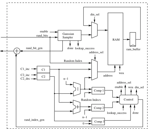
A hardware architecture for the secure consecutive-sampling is shown in Figure 7. In the architecture, C1 is an
up-counter and C2 is an up-down-counter. When the enable
signal is high, the Gaussian sampler generates samples in an iterative way. After generation of each sample, the signal
Gdone goes high and the type of the sample is indicated by the
signal lookup success. In the case when the sample has been generated using a successful lookup operation, lookup success becomes high. Depending on the value of the lookup success, the control machine stores the sample in the memory address C1or(n−C2)and also increments the corresponding counter.
Completion of then sampling operations is indicated by the output from Comparator2.
In the random-shuffling phase, a random address is gen-erated and then compared with (n −C2). If the
random-address is smaller than (n−C2)then it is used for the swap
operation; otherwise another random-address is generated. Now the memory content of address(n−C2)is swapped with
the memory content of random-address using the ram buffer register. After this swap operation, the counterC2 decrements
by one. The last swap operation happens whenC2 is zero.
VI. EXPERIMENTALRESULTS
Sampler Architecture ROM-width ROM-depth LU-depth LUTs FFs Slices BRAM Delay (ns) Cycles
Basic Knuth-Yao Sampler 24 128 - 101 81 38 - 2.9 17
Basic Knuth-Yao Sampler 12 256 - 105 60 32 - 2.5 17
Basic Knuth-Yao Sampler⋆ 6 512 - 102 48 30 - 2.6 17
Fast Knuth-Yao Sampler 6 512 8 118 48 35 - 3 ≈2.5
Knuth-Yao Sampler [7] 32 96 - 140 - 47 - 3 17
Bernoulli Sampler [11] - - - 132 40 37 - 7.3 144
Polynomial Sampler–1 6 512 8 135 56 44 1 3.1 392
Polynomial Sampler–2 6 512 8 176 66 52 1 3.3 420
TABLE III
PERFORMANCE OF THE DISCRETEGAUSSIAN SAMPLER ON XC5VLX30
are obtained from the Xilinx ISE12.2 tool after place and route analysis. In the table we show area and timing results of our architecture for various configurations and modes of operations and compare the results with other existing architectures. The results do not include the area of the random bit generator. Area requirements for the basic bit-scan operation based Knuth-Yao sampler for different ROM-widths and depths are shown in the first three columns of the table. The optimal area is achieved when the ROM-width is set to 6 bits. As the width of the ROM does not affect the cycle requirement of the sampler architecture, all different configurations have same clock cycle requirement. The average case cycle requirement of the sampler is determined by the number of bits scanned on average per sampling operation. A C program simulation of the Knuth-Yao random walk in [7] shows that the number of memory-bits scanned on average is 13.5. Before starting the bit-scanning operation, the sampler performs two column jump operations for the first two all-zero columns of the probability matrix (for σ = 3.33). This initial operation requires two cycles. After this, the bit scan operation requires 14 cycles to scan 14 memory-bits and the final transition to the completion state of the FSM requires one cycle. Thus, on average 17 cycles are spent per sampling operation. The most area-optimal instance of the Knuth-Yao sampler is smaller by 17 slices than the Knuth-Yao sampler architecture proposed in [7]. The effect of the bit-scan unit and decentralized control logic is thus evident from the comparison. The compact Bernoulli sampler proposed in [11] consumes 37 slices and spends on average 144 cycles to generate a sample point. Thus in comparison to the Bernoulli sampler, our Knuth-Yao sampler is both smaller and faster.
The fast sampler architecture in the fourth column of Table III uses a lookup table that maps eight random bits. The sampler consumes additional five slices compared to the basic bit-scan based architecture. The probability that a table lookup operation returns a sample is 0.973. Due to this high success rate of the lookup operation, the average case cycle require-ment of the fast sampler is slightly larger than 2 cycles with the consideration that one cycle is consumed for the transition of the state-machine to the completion state. In this cycle count, we assume that the initial eight random bits are available in parallel during the table lookup operation. If the random number generator is able to generate only one random bit per cycle, then additional eight cycles are required per sampling operation. However generating many (pseudo)random bits is not a problem using light-weight pseudo random number
generators such as the trivium steam cipher which is used in [11]. The results in Table III show that by spending additional five slices, we can reduce the average case cycle requirement per sampling operation to almost two cycles from 17 cycles. As the sampler architecture is extremely small even with the lookup table, the acceleration provided by the fast sampling architecture will be useful in designing fast cryptosystems.
The Polynomial Sampler–1 architecture in the seventh column of Table III generates a polynomial of n = 256 coefficients sampled from the discrete Gaussian distribution by using the fast sampler iteratively. The samples are stored in the RAM from address 0 to n−1. During the consecutive sampling operations, the state-machine jumps to the next sampling operation immediately after completing a sampling operation. In this consecutive mode of sampling operations, the ‘transition to the end state’ cycle is not spent for the individual sampling operations. As the probability of a successful lookup operation is 0.973, in the average case 249 out of the 256 samples are generated using successful lookup operations; whereas the seven samples are obtained through the sequential bit-scanning operation. In this consecutive mode of sampling, each lookup operation generated sample consumes one cycle. Hence in the average case 249 cycles are spent for generating the majority of the samples. The seven sampling operations that perform bit scanning starting from the ninth column of the probability matrix require on average a total of 143 cycles. Thus in total 392 cycles are spent on average to generate a Gaussian distributed polynomial.
The Polynomial Sampler–2 architecture includes the random shuffling operation on a Gaussian distributed polynomial of n= 256 coefficients. The architecture is thus secure against simple time and power analysis attacks. However this security comes at the cost of an additional eight slices due to the requirement of additional counter and comparator circuits. The architecture first generates a polynomial in 392 cycles and then performs seven swap operations in 28 cycles in the average case. Thus in total the proposed side channel attack resistant sampler spends 420 cycles to generate a secure Gaussian distributed polynomial of 256 coefficients.
VII. CONCLUSION
without affecting the cycle count. Moreover, in this paper we proposed a fast sampling method using a very small-area precomputed table that reduces the cycle requirement by seven times in the average case. We showed that the basic sampler architecture can be attacked by exploiting its timing and power consumption related leakages. In the end we proposed a cost-effective counter measure that performs random shuffling of the samples.
REFERENCES
[1] S. Rich and B. Gellman, “NSA Seeks to build Quantum Computer that could crack most types of Encryption,” The Washington Post, 2nd January, 2014, http://www.washingtonpost.com/world/national-security/. [2] O. Regev, “LatticeBased Cryptography,” in Advances in Cryptology -CRYPTO 2006, ser. LNCS, C. Dwork, Ed., vol. 4117. Springer Berlin, 2006, pp. 131–141.
[3] T. P ¨oppelmann and T. G ¨uneysu, “Towards Efficient Arithmetic for Lattice-Based Cryptography on Reconfigurable Hardware,” in Progress in Cryptology LATINCRYPT 2012, ser. LNCS, A. Hevia and G. Neven, Eds., vol. 7533. Springer Berlin, 2012, pp. 139–158.
[4] N. G ¨ottert, T. Feller, M. Schneider, J. Buchmann, and S. Huss, “On the Design of Hardware Building Blocks for Modern Lattice-Based En-cryption Schemes,” in Cryptographic Hardware and Embedded Systems CHES 2012, ser. LNCS, vol. 7428. Springer Berlin, 2012, pp. 512–529. [5] T. Frederiksen, “A Practical Implementation of Regev’s LWE-based Cryptosystem,” in http://daimi.au.dk/ jot2re/lwe/resources/, 2010. [Online]. Available: http://daimi.au.dk/ jot2re/lwe/resources/
[6] T. P ¨oppelmann and T. G ¨uneysu, “Towards Practical Lattice-Based Public-Key Encryption on Reconfigurable Hardware,” in Selected Areas in Cryptography – SAC 2013, ser. Lecture Notes in Computer Science. Springer Berlin Heidelberg, 2014, pp. 68–85.
[7] S. S. Roy, F. Vercauteren, and I. Verbauwhede, “High Precision Discrete Gaussian Sampling on FPGAs,” in Selected Areas in Cryptography – SAC 2013, ser. Lecture Notes in Computer Science. Springer Berlin Heidelberg, 2014, pp. 383–401.
[8] S. S. Roy, F. Vercauteren, N. Mentens, D. D. Chen, and I. Ver-bauwhede, “Compact Ring-LWE based Cryptoprocessor,” Cryptology ePrint Archive, Report 2013/866, 2013, http://eprint.iacr.org/. [9] A. Aysu, C. Patterson, and P. Schaumont, “Low-cost and Area-efficient
FPGA Implementations of Lattice-based Cryptography,” in HOST. IEEE, 2013, pp. 81–86.
[10] T. P ¨oppelmann, L. Ducas, and T. G ¨uneysu, “Enhanced Lattice-Based Signatures on Reconfigurable Hardware,” Cryptology ePrint Archive, Report 2014/254, 2014, http://eprint.iacr.org/.
[11] T. P ¨oppelmann and T. G ¨uneysu, “Area Optimization of Lightweight Lattice-Based Encryption on Reconfigurable Hardware,” in Proc. of the IEEE International Symposium on Circuits and Systems (ISCAS-14), 2014, Preprint.
[12] T. Oder, T. P ¨oppelmann, and T. G ¨uneysu, “Beyond ECDSA and RSA: Lattice-based Digital Signatures on Constrained Devices,” in Proceed-ings of the The 51st Annual Design Automation Conference on Design Automation Conference, ser. DAC ’14. New York, NY, USA: ACM, 2014, pp. 110:1–110:6.
[13] A. Boorghany and R. Jalili, “Implementation and Comparison of Lattice-based Identification Protocols on Smart Cards and Micro-controllers,” Cryptology ePrint Archive, Report 2014/078, 2014, http://eprint.iacr.org/.
[14] L. Ducas and P. Q. Nguyen, “Faster Gaussian Lattice Sampling Using Lazy Floating-Point Arithmetic,” in Advances in Cryptology ASI-ACRYPT 2012, ser. LNCS, vol. 7658. Springer Berlin, 2012, pp. 415– 432.
[15] D. E. Knuth and A. C. Yao, “The Complexity of Non-Uniform Random Number Generation,” Algorithms and Complexity, pp. 357–428, 1976. [16] L. Ducas, A. Durmus, T. Lepoint, and V. Lyubashevsky, “Lattice
Signatures and Bimodal Gaussians,” Cryptology ePrint Archive, Report 2013/383, 2013, http://eprint.iacr.org/.
[17] V. Lyubashevsky, “Lattice Signatures without Trapdoors,” in Proceed-ings of the 31st Annual international conference on Theory and Appli-cations of Cryptographic Techniques, ser. EUROCRYPT’12. Berlin: Springer-Verlag, 2012, pp. 738–755.
[18] N. Dwarakanath and S. Galbraith, “Sampling from Discrete Gaussians for Lattice-based Cryptography on a Constrained Device,” Applicable Algebra in Engineering, Communication and Computing, vol. 25, no. 3, pp. 159–180, 2014.
[19] L. Devroye, Non-Uniform Random Variate Generation. New York: Springer-Verlag, 1986. [Online]. Available: http://luc.devroye.org/rnbookindex.html
[20] V. Lyubashevsky, C. Peikert, and O. Regev, “On Ideal Lattices and Learning with Errors over Rings,” in Advances in Cryptology EU-ROCRYPT 2010, ser. Lecture Notes in Computer Science, vol. 6110. Springer Berlin Heidelberg, 2010, pp. 1–23.