Analysis of the Rainbow Tradeoff Algorithm
Used in Practice
Jung Woo Kim, Jin Hong, and Kunsoo Park
Abstract—Cryptanalytic time memory tradeoff is a tool for inverting one-way functions, and the rainbow table method, the best-known tradeoff algorithm, is widely used to recover passwords. Even though extensive research has been performed on the rainbow tradeoff, the algorithm actually used in practice differs from the well-studied original algorithm. This work provides a full analysis of the rainbow tradeoff algorithm that is used in practice. Unlike existing works on the rainbow tradeoff, the analysis is done in the external memory model, so that the practically important issue of table loading time is taken into account. As a result, we are able to provide tradeoff parameters that optimize the wall-clock time.
Index Terms—cryptanalytic time memory tradeoff, rainbow tradeoff, external memory model.
I. INTRODUCTION
T
HE rainbow tradeoff [35] is a generic and probabilistic method for quickly inverting a one-way function. In any cryptanalytic time memory tradeoff algorithm, such as the rainbow tradeoff, a large pre-computation table is generated through a massive one-time pre-computation phase that is specific to the one-way function under consideration, after which the inversion of each given target becomes much faster than an exhaustive search of inputs. Cryptanalytic tradeoff al-gorithms allow the implementer to balance the size of the pre-computation table against the time taken for each inversion, through appropriate choices of the algorithm parameters.Implementations of the tradeoff technique are actively used today by law enforcement agencies, system security managers, and hackers to recover passwords from unsalted password hashes. There are also many commercially available tools [1], [3], [5], [7], [8], based on the tradeoff technique, that can recover forgotten passwords protecting access to certain types of documents (PDF, MS Word, WinZip, and so on).
The first cryptanalytic tradeoff algorithm was presented by [23] and this was soon amended with the idea of using distinguished points [21], which greatly reduced the number of table lookup operations and made the algorithm much more practical for use. The rainbow tradeoff [35] is a more recent invention, which has received a lot of publicity [17], [19], [31], [32] for being able to “break Windows passwords.” There are numerous variants of the tradeoff algorithms we have already mentioned, each claiming to be superior over existing algorithms, but a quick search on the Web would reveal that
J. W. Kim and J. Hong are with the Department of Mathematical Sciences, Seoul National University, Seoul 151-747, Korea. K. Park is with the Depart-ment of Computer Science and Engineering, Seoul National University, Seoul 151-742, Korea.
the rainbow tradeoff is currently almost the only algorithm used, at least for the purpose of recovering passwords.
The cryptanalytic tradeoff algorithms have been imple-mented extensively on various platforms [18], [22], [26], [28], [33], [34], [37], [38], with some of the more recent implementations taking advantage of the massively parallel GPU platform. The rainbow tradeoff has its share of imple-mentations, with [2], [4], [6], [9] being a list of the current more prominent providers of pre-computed rainbow tables.
In this work, we focus on the discrepancy between the original rainbow tradeoff algorithm and its variants that are implemented and used in practice. The rainbow tradeoff, as with other tradeoff algorithms, was designed with the implicit assumption of a flat memory structure. In other words, the random access machine (RAM) model [20] of computation, where a machine consists of a central processing unit (CPU) and a single level of memory, was assumed.
However, in practice, the very large pre-computation tables of the rainbow tradeoff must initially reside on slow disks and these need to be loaded into smaller main memory for processing. This situation is quite different from the RAM model of computation and the highly non-localized memory access behavior of the original rainbow tradeoff makes its straightforward implementation on a modern computer quite impractical for use, except in the less interesting case of small search spaces. As far as rainbow tradeoffs are concerned, the external memory model [11], which takes two levels of memory into account, is a much more realistic view of modern computing systems than the RAM model of computation.
Current implementers of the rainbow tradeoff are well aware of the impracticality of the original algorithm and have chosen to implement slightly modified versions of the algorithm. The main operations of the original algorithm are retained, but the order of these operations are changed so that accesses to the pre-computed tables are done in a somewhat localized and sequential manner. This removes the need to transfer the same data multiple times from the slow disk to fast main memory and the algorithm is made much more suitable for use on real-world computers.
from being applied to the algorithm used in practice.
We further note that these previous analyses were carried out in the RAM model of computation. For example, the performance of the algorithm was measured in terms of the size of the pre-computation tables and the expected amount of one-way function computations. Such an approach ignores the fact that the main memory is a much more expensive resource than the disk and completely disregards the time taken for data transfers between disk and main memory. Hence, even if results analogous to the previous analyses were available for the rainbow tradeoff algorithms used in practice, these would not properly reflect the performance or characteristics of the rainbow tradeoff that practitioners would be interested in.
In this work, we analyze the performance of the rainbow tradeoff variant that is widely used in practice [4], [9]. Our analysis will be done in the external memory model, so that the algorithm characteristics of practical importance are captured, and this will bring forward a completely new type of tradeoff curve. Note that, because our model of computation and analysis capture even the disadvantage in table loading time associated with the use of a larger pre-computation table, we are able to consider theminimizationof the online time of the rainbow tradeoff variant, where the online time refers to the sum of the time taken for one-way function computations and the time taken for loading of tables. This was not previously possible, since time memory tradeoff in the RAM model somewhat erroneously implies that a larger pre-computation table will always bring about a smaller online time. Our analysis will conclude with the explicit tradeoff parameters that optimize the online wall-clock time.
The introduction of the classical Hellman algorithm [23] was accompanied with a very rough cost estimate of its hardware implementation. This was followed by early works that discussed the asymptotic effectiveness of the tradeoff techniques [12] in terms of monetary cost per inversion, or tried to minimize the hardware implementation cost [29] of the classical Hellman algorithm under an upper bound on the online computational complexity. A more recent article [39] discussed the asymptotic cost and computational complexity of the classical Hellman algorithm and its distinguished point variant, along with many other cryptanalytic algorithms. This was a highly theoretical work that represented the cost of a machine in terms of its number of components.
The rainbow tradeoff [35] was introduced after modern computers became widely available. The change in computing environment made the software implementations of the rain-bow tradeoff more popular, and the RAM model of computa-tion naturally became implicit in its theoretical analyses. The article [14] introduced the notion of tradeoff characteristic to discuss the advantage of one tradeoff algorithm over another and [25] brought the cost of pre-computation into considera-tion in comparing algorithm performances. Even though there are such articles that consider measures other than the storage size and online computational complexity in representing the performance of a tradeoff algorithm, these were still bound by the RAM model of computation.
To the best of our knowledge, the current article is the first to consider the rainbow tradeoff in the external memory model
of computation. In fact, this seems to be the first treatment of any cryptanalytic tradeoff algorithm in the external memory model.
The rest of the paper is organized as follows. In Section II, we explain the RAM and external memory models of computa-tion. The precise version of the rainbow tradeoff algorithm that will be analyzed in this paper is given in Section III, together with justifications for choosing to work with this specific algorithm. The rainbow tradeoff algorithm used in practice is fully analyzed in Section IV, where formulas for calcu-lating the optimal algorithm parameters are given. Section V illustrates our results with examples of optimal parameters. Test results supporting the correctness of our analysis is given in Section VI, and we conclude in Section VII. The less popular non-perfect table rainbow tradeoff is fully treated in the appendix.
II. MODELS OFCOMPUTATION
There are two representative models that are used to describe modern computers. These are the random access machine (RAM) model and the external memory model.
RAM Model: In the RAM model, the computer is assumed to consist of a central processing unit (CPU) and a storage unit of infinite capacity. The storage is assumed to allow accesses to any of its location in unit time, even if the locations are chosen in a random manner. This model is useful in predicting the real behavior of modern computers, as long as the amount of data processed is smaller than the size of the main memory of the computer.
Previous analyses [14], [24], [25], [30], [35] of the rainbow tradeoff have always been in the RAM model of computation. Some of these analyses completely ignored the cost of table lookups. Others claimed that the time taken for table lookups would be insignificant in comparison to the time taken for computations of the one-way functions. This claim was based on the observation that the number of table searches were of much smaller order than the number of one-way function computations, but this reasoning becomes problematic when each table search take much longer than a single iteration of the one-way function. Results from these previous analyses are correct and useful when the complete set of pre-computation tables can be preloaded into the computer’s fast main memory so that table searches are indeed easy. However, they have very limited applicability when the size of the pre-computed data is so large that accesses to slower storage media become inevitable.
The discussion so far indicates that the analyses of the rainbow tradeoff algorithm done in the RAM model have very limited applicability to the use of rainbow tradeoff seen in practice, especially when the search space is large enough to call for the use of very large pre-computation tables.
External Memory Model: The architecture of modern com-puters are much more complex than what is suggested by the RAM model. In particular, modern computers have a hierarchy of memory units, some of which would be registers, caches, main memory, disk storage, and removable storage media. We wish to focus on the fact that, on real-world computers, when the size of data to be processed by a program is very large and accesses to the data are not localized, the data transfers between the main memory and the disk often become the largest performance bottleneck.
The external memory model [11] assumes a machine that consists of a CPU and two levels of memory. The capacity of the slower memory is assumed to be infinite, whereas that of the faster memory is taken to be bounded. This is a reasonable view of the modern computer, with the main memory and the disk taken to be the two levels of memory.1 The low price of disk storage today justifies the treatment of the slower memory as being unbounded in capacity. Data is transferred between the two memories in units of blocks.
In this work, we study the performance of the rainbow tradeoff in the external memory model. Since the disk space required for the long-term storage of pre-computation tables is assumed to be unlimited in size, our focus will be on how the online time can be minimized. Here, the online time refers to the wall-clock time, consisting mainly of the time taken to compute the one-way functions and the time taken to transfer data between disk and main memory. This concept of online time should not be confused with the online computational complexity, which most analyses on any time memory tradeoff algorithm would concentrate on.
III. RAINBOWTRADEOFFALGORITHMUSED INPRACTICE
In this section, we explain the differences between the original rainbow tradeoff algorithm [35] and its variant that is widely used in practice [4], [9]. The two rainbow algorithms will be referred to as the ThRb (theoretical) and PrRb (practical) algorithms in this paper. The reader is assumed to be familiar with the general framework of the rainbow tradeoff algorithm, although we will review the terminology and fix notation below.
We focus on the perfect table version of rainbow tradeoff, which is known to be more efficient in the online phase than the non-perfect table version. The one-way function to be inverted, such as the password hash function, will be written as f, and its composition with thei-th reduction function ri will be denoted by fi =ri◦f. The size of the search space (domain off) will be written asN. As is usual, symbolsm,t, and`will be used to represent the number of entries per pre-computation table, the length of each pre-pre-computation chain,
1The cache memory (cache-oblivious model [36]) is not treated separately
in this work. The memory access characteristics of the rainbow tradeoff variants are such that no meaningful performance improvement can be expected from cache memory considerations.
and the number of tables, respectively. Reasonable parameter choices would satisfymt≈N. The matrix stopping constant
is defined to be¯c=mtN, and it is known [13], [14], [24] that
¯
c<2, for perfect tables.
Pre-computation Phase: The ThRb and PrRb algorithms are identical in their computation phases. During the pre-computation phase, chains of the form
SPi f1
−−−→ ◦ f2
−−−→ ◦ · · · ◦ ft
−−→EPi, (1)
are generated from multiple starting points, and the start-ing and endstart-ing point pairs (SPi,EPi) are stored in a pre-computation table, after being sorted on the ending points. Only one entry is stored from any set of chains with identical ending points, so that usually more thanmchains need to be generated in creating each table. This is the only difference between a perfect table and a non-perfect table. The set ofm
chains corresponding to each pre-computation table is referred to as the pre-computation matrix. The reader is cautioned to distinguish between a computation table and a pre-computation matrix, while reading the rest of this paper. The table creation procedure is repeated with distinct sets of reduction functions to produce`pre-computation tables.
Perfect versus Non-perfect Tables: The currently available offerings of the rainbow tradeoff tables on the Web indicate that the perfect tables are being somewhat favored over the non-perfect tables, at least by those that are using the rainbow tradeoff in practice.
Pre-computation tables available through the WebTables paid service from Cryptohaze [2] are perfect tables. Free Rainbow Tables [4] only releases perfect tables and makes it clear that they advocate the use of perfect tables. The tables freely available from ophcrack [6] are also perfect tables and this indicates that their larger tables, commercially available from Objectif S´ecurit´e, are also perfect tables.
RainbowCrack Project [9] is an exception, as they sell non-perfect tables. However, they provide tools for converting the non-perfect tables to perfect tables, with a warning stating that the conversion wastes very expensive pre-computation effort. Based on these observations, we focus in the perfect table version of the rainbow tradeoff in this article. However, an equally complete analysis of the non-perfect table case is pro-vided in the appendix, for those interested in taking advantage of its lower pre-computation cost. The appendix also includes a very preliminary comparison between the perfect and non-perfect table versions of the rainbow tradeoff.
Online Phase in General: The only differences between ThRb and PrRb algorithms are in their online phases. Let the inversion target be given as y = f(x), where x is the unknown answer one is aiming to obtain. An online chain of length kis a chain of the form
x−−−−→ft−k+1
rt−k+1(y)
ft−k+2
−−−−→ ◦ · · · ◦ ft
−−−−→ ◦. (2)
Our convention is to include the unknown answer x in the online chain when stating its length, so that chain lengths k
specific pre-computation table, so that every online chain is associated with a specific pre-computation table. There are t
online chains, for each of the `tables.
With both the ThRb and PrRb algorithms, whenever an online chain is generated, its ending point is searched for among the ending points recorded in its corresponding pre-computation table. If a match of ending points is discovered, one retrieves the corresponding starting point and regenerates the pre-computation chain to the correct length. One hopes for this operation to reveal the correct answer x, but because the one-way functionf is not injective, most of these matches result from merging of chains, and these are identified as false alarms.
Online Phase ofThRb: The main difference betweenThRb andPrRbalgorithms is in theorderin which the online chains are generated. In the ThRb case, all shorter online chains are generated before any longer chains. More specifically, the following approach is taken.
Algorithm 1 Online Phase of ThRb
1: fork= 1 tot do 2: fori= 1 to` do
3: generate length-konline chain fori-th table
4: search for matching ending point ini-th table
5: ifmatch is foundthen
6: regenerate pre-computation chain
7: end if
8: ifanswer is foundthen
9: exit from all loops and terminate
10: end if
11: end for
12: end for
This ordering of online chain generation is often referred to as the parallel processing of the pre-computation tables.
Note that the probability for each online chain to lead to the discovery of the correct inversion answer is independent of the chain length. Since one expects to terminate the algorithm with the correct inversion answer before generating all t` online chains, dealing with the shorter chains before the longer chains is expected to be advantageous in terms of computational cost. This reasoning may seem plausible, but, in practice, one must also take into consideration the time required for table lookups. When the size of the fast main memory is smaller than the space required to hold the complete set of pre-computation tables, the approach ofThRbwould call for fre-quent non-sefre-quential accesses to the disk, which is something many implementers would try to avoid.
Online Phase of PrRb: One wishes to tweak the rainbow tradeoff algorithm so that the same pre-computation table information need not be loaded multiple times from slow storage to fast memory. Switching the order of the first two lines in the online phase ofThRb, i.e., the twoforstatements, is a reasonable solution when each pre-computation table fits within the main memory, and this is often referred to as the sequential processing of the pre-computation tables. However, since we are mainly interested in the situation where even the
size of each pre-computation table is much larger than the available main memory, further measures are necessary.
To execute the online phase of PrRb, one first decides on a splitting of each pre-computation table into s sub-tables. The integer s is chosen so that each sub-table, which contains ms entries, fits comfortably within the available main memory. In processing each pre-computation table, thetonline chains for that table are first generated. Then, each sub-table is loaded into fast memory, in turn, and all searches and resolving of false alarms associated with the loaded sub-table are performed before the next sub-table is loaded.
Explicitly, the following steps are taken.
Algorithm 2 Online Phase ofPrRb
1: fori= 1to `do
2: fork= 1to tdo
3: generate length-k online chain fori-th table
4: record the online chain ending point
5: end for
6: forj= 1 to sdo
7: loadj-th sub-table of i-th table
8: fork= 1to tdo
9: retrieve recorded ending point of length-k online chain
10: search for matching ending point in loaded sub-table
11: if match is foundthen
12: regenerate pre-computation chain
13: end if
14: if answer is foundthen
15: exit from all loops and terminate
16: end if
17: end for
18: end for
19: discard recorded online chain ending points
20: end for
Note that the temporary recording of the online chain ending points must be done to fast main memory. Since any reasonable rainbow parameters would satisfy t √N, this will not cause any practical difficulties, whenNis of size for which the pre-computation can be handled.
Appropriateness of studying PrRb: Let us briefly explain that the PrRb algorithm is the appropriate online phase algorithm to study in view of practical usefulness. No two implementations of the rainbow tradeoff can be exactly the same, but the above PrRb algorithm is roughly what is implemented by both RainbowCrack Project [9] and the online phase programrcracki_mt[10] that is to be used with the tables freely available from Free Rainbow Tables [4]. Hence PrRbis indeed widely used in practice.
index files loaded in main memory. Even though they use some interesting techniques, such as the separate storing of starting and ending points, frequent searches to the disk can only leave the CPU idle, and is likely to result in inefficient use of system resources.
The ThRbalgorithm is more efficient than thePrRb algo-rithm, when the combined size of the pre-computation tables is small, so that the RAM model is applicable. We acknowledge that, when the search space is immensely large, there is possibility for the direct disk search approach, combined with a more sophisticated hash table structure, to be reasonable. However, for large search space sizes that can be processed today by commercial entities or through distributed computing on volunteered CPU cycles, the PrRb approach seems to be more plausible.
Cryptohaze [2], the remaining major provider of pre-computed rainbow tables, only distributes a GPU implemen-tation of the online phase. In fact, both rcracki_mt and the online phase program of RainbowCrack Project contain supports for GPU use. However, characteristics of compu-tations and memory accesses done on a GPU platform are quite different from those associated with a single core or a small number of cores, and the rainbow tradeoff executed on these GPU platforms require a completely separate analysis. Analysis of the rainbow tradeoff specific to the GPU platform is clearly an interesting subject of study, and the current article should be a good starting point for such an attempt.
IV. ANALYSIS IN THEEXTERNALMEMORYMODEL
In this section, we analyze the performance of PrRb, the rainbow tradeoff algorithm that is used in practice. The exact details of the algorithm were explained in Section III.
Our goal is to minimize the expected online wall-clock time for solving an inversion problem. In dealing with the rainbow tradeoff algorithm in the external memory model, there are two major components that constitute the online time. These are the time required for computations of the one-way function and the time required to load pre-computation table from slow disk storage to fast main memory. There are other smaller issues, such as the time taken to perform table lookups within data that is already residing in fast memory, but these should be small enough to be ignored. To achieve our goal, we will need to obtain the expected online computational complexity and the amount of pre-computation table that is expected to be loaded into main memory during the online phase.
During our analysis we will frequently write very accurate approximations as equalities. The two most common such approximations are applications of 1 − 1
a
b
= e−ba and
definite integral expressions for large summations.
Recall that disk reads are usually performed in units of
blocks. In the remainder of this article, we assume each block containsβ pre-computation table entries.
For the sake of clarity, the notation used for the tradeoff parameters are summarized in Table I.
Some Probabilities of Failure: We start by writing down a few probabilities of failure at various stages of the online phase. It is quite straightforward to argue as in [13], [14], [35]
TABLE I
NOTATION FOR ALGORITHM PARAMETERS.
Symbol Meaning
N size of search space m number of chains per table
t length of chains
` number of tables
s number of sub-tables per table
that the online processing of a single perfect rainbow table, constructed with parameters m and t, will fail to return the correct inversion answer with probability
1−m
N
t
=e−mtN =e−¯c, (3)
and this implies that the probability for all pre-computation tables before thei-th one not to contain the inversion answer is
n
1−m
N
toi−1
=e−(i−1)¯c. (4)
A trivial corollary would be the probability of success [35]
¯
Rps= 1−e−¯c`, (5)
for the full online phase. Similarly, the probability for the correct inversion answer not to be found in the first j −1
sub-tables of a pre-computation table is
1−(j−1)m sN
t
=e−j−s1¯c, (6)
and the similar probability of failure for the first j−1 sub-tables and the first k−1 columns of the j-th sub-table that are closest to the ending column in a pre-computation table is
1−jm sN
k−1
1−(j−1)m sN
t−k+1
=e−js k−1
t ¯ce− j−1
s t−k+1
t ¯c=e− k−1
t ¯sce− j−1
s ¯c.
(7)
The probabilities stated above are at the core of all proofs for the claims to be given below.
Supporting Claims: Our first statement presents the average usage of the pre-computed data.
Proposition 1. During the online phase of the perfect rainbow tradeoff, one can expect
L= 1−e
−¯c`
1−e−¯cs m sβ
blocks of pre-computation table data to be loaded into main memory and searched for collisions with the online chains. Whensis sufficiently large,
L=1−e
−¯c`
¯
c
m β
is a good approximation.
to (4) and (6), the number of loaded blocks may be counted as ` X i=1 s X j=1
e−(i−1)¯ce−j−s1¯c m sβ =
1−e−¯c`
1−e−¯c
s m sβ.
The second claim is thes→ ∞limit of the first claim. Note that 1
1−e−¯sc
¯c s = 1 +
1 2 ¯c s+O(
¯c s
2
), so that this approximation is quite accurate for even moderately large s.
Our next goal is to find the computational complexity of the online phase. This is broken into to the online chain generation part and the false alarm resolving part.
Lemma 2. The generation of the online chains is expected to require
1−e−¯c`
1−e−¯c
t2
2
iterations of the one-way function.
Proof: The batch of t online chains for the i-th pre-computation table, which requires approximately t22 one-way function iterations to create, will be generated if and only if all previous i−1 pre-computation tables did not contain the correction inversion answer. Referring to (4), the number of one-way function iterations associated with the generation of online chains can be written as P`
i=1e
−(i−1)¯c×t2
2, which is
what is claimed.
The remaining online computational complexity associated with false alarm resolving may be treated similarly, except that the calculations are slightly more complicated.
Lemma 3. The resolving of false alarms is expected to require
1−e−¯c` 1−e−¯sc
2(3s−4)−(s−2)¯c s
−2(3s−4) + (4s+ ¯c−4)¯c s
e−¯sc
s ¯ c
2t2
4
iterations of the one-way function. Whensis sufficiently large
1−e−¯c`1 6− ¯ c 48 t2
is a good approximation.
Proof:According to Proposition 4 of [24], the probability for an online chain of lengthkto merge into a perfect rainbow matrix consisting ofmending points is m(kN+1)1−mk
4N
. The probability for an online chain to merge into any sub-table of
m
s chains would be
1
s of this. Now, referring to (4) and (7), the work expected from resolving alarms may be written as
` X i=1 s X j=1 t X k=1
(t−k+ 1)×1 s
m(k+ 1)
N
1−mk
4N
×e−(i−1)¯ce−k−t1 ¯c
se− j−1
s ¯c.
After the iandj summations are separated, we have
1−e−¯c`
1−e−¯c
1−e−¯c
1−e−¯sc
×
t
X
k=1
(t−k+ 1)×1 s
m(k+ 1)
N
1−mk
4N
×e−k−t1 ¯c
s.
The remaining summation may be approximated by a definite integral and the above becomes
1−e−¯c` 1−e−¯sc
¯ c st 2 Z 1 0
(1−x)x1−¯c
4x
e−¯scxdx.
What is stated is the result of explicitly calculating this definite integral.
The second statement follows from an easy verification of
1 1−e−¯cs
. . . s
¯c 2 1 4 = 1 6 − ¯ c 48+ ¯c 480 ¯ c s+O(
¯c s
2
). Here, the
constant hidden behind the big-Onotation does depends on¯c, but does not depend ons. This also indicates the accuracy of the approximation.
The computational complexity of the online phase is now a direct consequence of the previous two lemmas.
Proposition 4. The online phase of the perfect rainbow tradeoff is expected to require
F = 1−e
−¯c`
1−e−¯sc t2 × 1 2
1−e−¯sc 1−e−¯c +
1 4 s ¯c 2 ×
2(3s−4)−(s−2)¯c s
−2(3s−4) + (4s+ ¯c−4)¯c s
e−¯sc
iterations of the one-way function. This includes both the cost of generating the online chains and the cost of resolving alarms. Whensis sufficiently large,
F = 1−e−¯c` 1
2(1−e−¯c)+
1 6 − ¯c 48 t2
is a good approximation.
We have thus acquired complete knowledge of both the computational complexity and the pre-computation table load-ing behavior of the rainbow tradeoff algorithm.
Main Results: The following statement is a direct conse-quence of Proposition 1 and Proposition 4.
Proposition 5. The expected number of blocks containing pre-computation table data loaded into main memory L and the expected number of one-way function iterations F for the perfect rainbow tradeoff used in practice satisfy the tradeoff curve
L2F = ¯RtcN2,
where the tradeoff coefficient is
¯
Rtc=1−e
−¯c`
1−e−¯sc
3 1 β2 × 1 2
1−e−¯cs 1−e−¯c
¯c s 2 +1 4
2(3s−4)−(s−2)¯c s
−2(3s−4) + (4s+ ¯c−4)¯c s
e−¯sc
.
Whensis sufficiently large
¯
Rtc= 1−e−¯c`
3 1
β2
1
2(1−e−¯c)+
is a good approximation of the tradeoff coefficient.
The original rainbow tradeoff algorithmThRballows trade-offs of the formM2F ≈N2to be performed, whereM is the
size of the required long-term storage (M = m`) and F is the number of one-way function iterations expected during its online phase. In fact, it can be shown that such a tradeoff curve is valid even for the rainbow tradeoff variant that is being considered here. However, since we are working in the external memory model, the long term storage size is no longer of interest.
Assuming the use of a modern multi-core CPU, it should be possible to tweak the PrRb algorithm, so that the sub-table loading and the one-way function computation operations are performed, at least in part, simultaneously. However, the corresponding programming is quite nontrivial, and the current implementations [4], [9] do not incorporate such an approach. Hence, the average wall-clock time for the online phase may be expressed as
T =τLL+τFF, (8)
whereτL andτF denote the average wall-clock time required to load a single block of pre-computation table data into main memory and the average wall-clock time taken by a single one-way function application, respectively.
Our next goal is to minimize the expected online time (8), by locating the appropriate balance between the valuesLand
F, which must adhere to the tradeoff curve of Proposition 5.
Theorem 6. Let the success rate requirementRps¯ and the pre-computation table count ` be such that ¯c=−ln(1−R¯ps)
` <2.
Let s and β be given and set Rtc¯ to the tradeoff coefficient computed through Proposition 5, using the given `, s, andβ values and the ¯cvalue we have just defined.
The online wall-clock time of the perfect rainbow tradeoff that achieves success rateR¯ps, uses` pre-computation tables,
and divides each table intos sub-tables can be minimized to
T = 3 223
τ23
Lτ
1 3
FR¯
1 3
tcN
2 3,
with
L=2τF τL
13¯
R13
tcN
2
3 and F =
τL
2τF
23¯
R13
tcN
2 3.
The above remains true whensis sufficiently large, as long as the tradeoff coefficient Rtc¯ of Proposition 5 corresponding to such a case is used.
Proof: Let us assume a fixed s and a fixed requirement
¯
Rps on the success rate of inversion, throughout this proof. When (5) is rewritten in the form¯c=−ln(1−R¯ps)
` , it becomes clear that, if the given success rate is to be met, the matrix stopping constant¯cthat must be used is completely determined by the number of tables`one chooses to use. Hence, under the fixed sandR¯ps, the choice of` fully determines the tradeoff coefficientRtc¯ , given by Proposition 5.
It is now straightforward to minimize the online time, separately for each choice of`, under the restriction placed by the tradeoff curve of Proposition 5. It suffices to substitutes
F = ¯RtcN2
L2 into (8), the expression for online time, and
minimize the resulting equation as a function of L.
Computing the Optimal Parameter Set: Given L and F
satisfying the tradeoff curve L2F = ¯R
tcN2, together with the corresponding `, ¯c, s and β, the explicit parameters that achieve these average behavior can be calculated from Proposition 1 and Proposition 4. In fact, recalling the definition of the matrix stopping constant, we can even write
m= 1−e
−¯c
s
1−e−¯c`sβL and t=
¯c N
m. (9)
When a sufficiently large sis assumed, the algorithm param-eters can be computed directly from¯cthrough the formulas
m=βτF τL
13 1
1−e−¯c +
1 3 −
¯c
24
13
¯c N23, (10)
t= τL βτF
13 1
1−e−¯c +
1 3 −
¯c
24
−13
N13. (11)
Thus, Theorem 6 allows us to obtain the parameters that minimize the online time, for each choice ofsand`. It now remains to discuss the optimal choice of s and `. A fixed requirement on the success rate Rps¯ is assumed throughout the discussion below.
Recall that each choice of`completely determines¯c. Hence, the tradeoff coefficientRtc¯ of Proposition 5 can be understood as a function of the single variable s, for each fixed `, and one can check through a quick 3D plot thatR¯tcis a decreasing function of s, for each fixed¯c. Since the online timeT is a constant multiple ofR¯
1 3
tc, using a largersis always better. Note that the proofs of our claims show that when any specific-sformula is approximated by a large-sformula, one will experience an error rate of roughly O 1
s
-order. This implies that taking s = 100 will be sufficient to make any differences unnoticeable. On the other hand, this also shows that even ifs is increased very far beyond, say,s= 100, the additional reduction in online time to be experienced will be very small.
We can even provide a heuristic argument to advocate the use of small sub-tables. The sub-table that was loaded just before the online phase returns the correct answer and terminates would not have been used as fully as the previous sub-tables. That is, if each sub-table size is very large, much of the data contained in the final sub-table to be processed would have been loaded into main memory in vain. Hence, it is advisable to increasesand reduce the size of each sub-table. In practice, making the sub-tables too small could bring about negative effects. Since disk read operations are ineffi-cient when done in sizes that are too small, one should not take the extreme approach of setting s = m and treat each table entry as a separate table. One should choose the sub-table size to be sufficiently large, so that the average speed of the segmented reading is sufficiently close to that expected of reading a very large file. However, considering the fact that filesystem block sizes are in the few KBs range, this minimum bound condition should never interfere with making
ssufficiently large.
TABLE II
PARTIAL INFORMATION ON THE OPTIMAL PARAMETERS FOR THE PERFECT RAINBOW TRADEOFF USED IN PRACTICE. USE OF A LARGEsIS ASSUMED.
¯
Rps ` ¯c β2R¯tc R¯pc
70% 1 1.20397 0.293563 3.02495 80% 1 1.60944 0.388166 8.24165 86.4% 1 1.99510 0.453935 814.392 90% 2 1.15129 0.637087 5.42610 95% 2 1.49787 0.668294 11.9320 98.1% 2 1.98166 0.665877 432.161 99% 3 1.53506 0.749060 19.8096 99.5% 3 1.76611 0.722067 45.3052 99.7% 3 1.93638 0.704215 182.623 99.9% 4 1.72694 0.736620 50.5949
searches and thus increasing the number of memory lookups. However, searches within data that already resides in main memory should take very little time and this increase should be ignorable. Furthermore, since the whole pre-computation table is sorted before it is divided into sub-tables, the extra memory lookups can be removed by sorting thetonline chain ending points and searching for the online ending point only in the appropriate sub-table.
Now that the use of an appropriately largesis justified, we can choose to work with the tradeoff coefficient
¯
Rtc=
¯
R3ps
β2
1
2(1−e−¯c)+
1 6−
¯
c
48
(12)
that does not involve s. It is easy to check that this is a strictly decreasing function¯cfor a fixedβ. Hence, to minimize the online time T, the largest possible ¯c = −ln(1−¯Rps)
` , or, equivalently, the smallest possible`, must be used, except that the condition ¯c < 2 must always be adhered to [13], [14], [24].
In summary, the online wall-clock time of the perfect rainbow tradeoff that achieves success rate R¯ps can be min-imized by using the smallest positive integer ` that satisfies
¯
c=−ln(1−R¯ps)
` <2, together with the correspondingmandt calculated through (10) and (11). Thesshould be chosen to be sufficiently large, but not so large that it decreases the speed of data transfer between the disk and main memory.
We have thus obtained explicit procedures and formulas for obtaining rainbow tradeoff parameters that are optimal, given any disk read speed, one-way function computation speed, and success rate requirement. Since the optimal table count`and the matrix stopping constant ¯c depends only on the success rate and not on the implementation platform, we have listed them in Table II for some success rates of interest.
The optimal values for the parametersm andt, which are not listed in the table, depend on the system constants τL andτF, and hence must be newly computed for each system through (10) and (11). The final column of the table contains the pre-computation coefficient, computed through the formula
¯
Rpc=
2¯c`
2−¯c, (13)
found in [30]. This is the number of one-way function it-erations, in multiples of N, that are required to produce the pre-computation table achieving the given success rate.
Miscellaneous Remarks: It should be understood that the optimality considered in this paper refers to the minimization of the online wall-clock time. In certain cases, the use of optimal parameters could require the cost of pre-computation to become prohibitively large. For example, it is possible to achieve the success rate of 86.4% with a single pre-computation table, but this requires¯c= 1.9951to be used and
813.39N iterations of the one-way function to be computed during the pre-computation phase. In such a case, one may choose to work with a slightly larger table count `, which would result in a slightly less efficient online phase.
Another point to note is that, by choosing to work in the external memory model, we have completely ignored the size of the required long-term storage. This is quite reasonable even in practice, as the low costs of hard disks and external storage units make the storage size requirement of much less practical importance than the online time. Nevertheless, since it can be shown that the storage size M and the expected number of blocks containing pre-computation table data loaded into main memoryLare connected through the relation
L=− Rps¯ βln(1−R¯ps)
M, (14)
we know that the minimization of (8), the online time, will automatically hold back the storage sizeM to within a man-ageable range, for any reasonable success rate requirement.
V. OPTIMALPARAMETEREXAMPLES
In this section, we provide two examples of optimized parameter sets. We use explicit realistic numbers and work with both a very large search space and a very small search space.
Constants: Let us first present the system constants. Our online machine consisted of an Intel i5 2.53GHz quad-core CPU, a 4GiB DDR3 main memory, and a 500GB 7200 RPM SATA hard disk drive. To work with realistic speed constants, we downloaded and made measurements using the online phase program rcracki_mt[10] and a sub-table from [4]. The 448.70MiB size sub-table, consisting of 226 entries, had
been created with the cryptographic hash function MD5 as the one-way function. Each sub-table entry takes 7 bytes of disk storage, with the decimal part of 448.70226×220 = 7.0110
coming from the index structure stored within the sub-table file. The block size of our filesystem is 4KiB, so that each block containsβ =74.×0110210 = 584.23table entries.
Using rcracki_mt and averaging over 5×10¹⁰ MD5 applications, we found that our machine required τF =
9.8195×10⁻⁸ seconds per one-way function iteration. The
speed of loading the sub-table from the disk to main memory, averaged over 180 trials, was τL = 8.5368×10⁻⁵ seconds per loading of pre-computation table data of a block size. We clarify that, to expedite table searches, rcracki_mt
expands each 7-byte pre-computation table entry into 16 bytes as it loads the table into main memory and that the stated measurement includes the time taken for this process.
considered all passwords that are at most eight characters in length. This was taken to be our search space, which is of size N=P8
i=195
i= 6.7048×1015= 252.574.
Our next steps concern Proposition 5 and Theorem 6. To obtain the success rate of Rps¯ = 99%, one must use ` = 3 pre-computation tables, together with parameters m and t
satisfying
mt
N = ¯c=−
ln(1−Rps¯ )
` = 1.5351. (15)
The success rate of 99% cannot be reached with less than 3
pre-computation tables, so that`= 3is the optimal number of tables to use. After calculating the tradeoff coefficient Rtc¯ = 0.74906 from the large-s formula of Proposition 5, we find that the average wall-clock time of the online phase can be minimized to
T =7811 sec=2 hr 10 min 11 sec, (16)
with the sub-table loadings and one-way function computa-tions taking
τLL=5207 sec and τFF=2604 sec, (17)
respectively.
The tradeoff parameters need to be set to m = 5.5257×
1010 = 235.685, t = 1.8626×105 = 217.507, and ` = 3,
for the stated optimal online performance and the success rate
¯
Rps= 99%to be obtained. We assume 2GiBs of our system’s 4GiBs of main memory are available for table loading. At
16 bytes per table entry, this amounts to 2×16230 = 227 table entries, so that each pre-computation table must be divided into at least 5.5257227×10¹⁰ ≈411.70sub-tables. This is already a
large number, so that the effect of increasingsany further will be negligible in reducing the online time, and we somewhat arbitrarily choose to take s= 450.
The s to be used is sufficiently large, but to verify that our approximations did not introduce unreasonable error, let us substitute the parameters m, t, `, ands into the formula of Proposition 5 that contain the parameter s and into the formulas of Theorem 6. We find that T(s=450) = 7820 sec, τLL(s=450)=5213 sec, andτFF(s=450)=2607 sec are quite
close to the previous large-s approximations given by (16) and (17).
Small Search Space Example: Let us next consider the example of a very small search space. We take the upper and lower case alphabets as our character set and consider all passwords of length 7, so that our search space is of size N= 527= 239.903.
To reach the success rate of R¯ps = 99.9%, one must use
` = 4 pre-computation tables with ¯c= 1.7269. The large-s
version of the tradeoff coefficient isR¯tc= 0.73662, and further calculations show that the optimal performance of
T =22.252 sec, τLL=14.835 sec, τFF =7.4174 sec (18)
can be achieved with parameters m = 1.7550×10⁸, t =
1.0116×10⁴,`= 4, and a large s.
At 16 bytes per table entry, each table requires 16m = 2.8080 × 109 bytes, to be loaded into main memory. A large portion of this could fit within our system’s 4GiB main
memory, but certainly not all ` = 4 pre-computation tables can be loaded into main memory simultaneously, so that we cannot run the ThRb algorithm on these pre-computation tables. Choosing to uses= 64, which is large enough to make our large-s computations sufficiently accurate, we can divide each pre-computation table into sub-tables of 41.843MiB size, which is more than large enough to prevent visible degradation of disk read speed.
ThRbversus PrRb: Since the ThRbalgorithm was men-tioned during our discussion of the small search space exam-ple, let us present a brief comparison under the setting of the example. Referring to Theorem 17 of [30], we can state that theThRballows tradeoffs of the form
M2F = 8.3915N2, (19)
whereM refers to the number of table entries. The tradeoff coefficient8.3915has been calculated from the values `= 4
and¯c= 1.7269, which are optimal for even the ThRbcase, under theRps¯ = 99.9% requirement.
At 16 bytes per table entry, at mostM =3×230
16 table entries
can be loaded into our system’s main memory, assuming 3GiBs of the 4GiBs were freely available. Thus, at least
F = 8.3915M2N2 = 2.1882×10
8 iterations of the one-way
function, which translates to T = τFF = 37.519 seconds, are required during the online phase of ThRb, assuming the pre-computation tables are pre-loaded into main memory. This is worse than the PrRb performance given by (18), but still somewhat comparable. In fact, if we assume that each table entry taking 7 bytes of disk space is expanded more carefully into only 8 bytes, rather than 16 bytes, of main memory space, with no changes toτL or τF, we arrive at the opposite conclusion, with PrRb taking 22.252 seconds and ThRbtaking 9.3796 seconds.
When dealing with small search spaces, neither the ThRb algorithm nor thePrRbalgorithm is at a clear advantage over the other. The choice of which to use must be made in a case by case manner based on many factors, such as the speed of one-way function computation, the speed of data transfer between disk and main memory, the size of main memory, and the required success rate. However, when large search spaces are under consideration, the use of ThRb algorithm can no longer be practical. Furthermore, even if theThRbalgorithm were to be executed, with frequent accesses to slow disk, the currently available analyses ofThRbwould have very limited success in predicting its online phase running time.
VI. EXPERIMENTALRESULTS
In this section, we show the results of our experiments done with thePrRbalgorithm. To be as objective as possible, we downloaded and used the executables and pre-computed rainbow tables from Free Rainbow Tables [4], and used them in verifying the correctness of our analyses.
space size is N = P7
i=195
i = 7.0577×1013 = 246.004.
The tables had been created and divided into sub-tables2using parameters
m= 45×226, t= 40000, `= 4, ands= 45, (20)
which corresponds toRps¯ = 99.89% and¯c= 1.7116. Our online system of speed characteristics τF = 9.8195×
10−8 and τ
L = 8.5368×10⁻⁵ was explained at the start of Section V. Using the downloaded executable, we ran the online phases on 200 randomly generated password hashes. Each run of the program displayed information labeled as “total disk access time”, “total cryptanalysis time” (false alarm treatment), and “total pre-calculation time” (online chain generation). We took the sum of the latter two as the time spent on one-way function computations. The average times for the 200 experiments, during which 99.5% of the hash values were successfully inverted, were
disk: 281.73 sec and comp: 118.09 sec, (21)
and this amounts to total timeT =399.82 sec. These are in good agreement with the values
τLL=262.47 sec, and τFF =116.35 sec, (22)
predicted by the s = 45 cases of Proposition 1 and Propo-sition 4. The small difference between theory (22) and prac-tice (21) can be explained by the fact that we have ignored the time taken for table searches. However, the difference is rather small, and the experiment confirms that there is no large overhead that has not been taken into account by our analysis. Let us briefly discuss the optimal parameters. For success rate R¯ps = 99.89%, the use of`= 4 is optimal, and we can calculate from (10) and (11) that the other parameters need to be set tom= 2919352791 andt= 41379. Incidentally, these are quite close to the parameters (20), used by our test table that was downloaded from Free Rainbow Tables.
Note that (10) and (11) imply that, for any fixed requirement on the success rate, optimal parameters mandtdepend only on the ratio τL
βτF. Hence, anyone who wishes to create rainbow
tables to be used by others, should first investigate into the approximate range of this ratio measured on the targeted users’ online phase systems.
VII. CONCLUSION
The performance of the rainbow tradeoff variant that is widely used in practice, as opposed to the well-studied original version, was analyzed in this paper. This was done in the external memory model, so that issues of practical relevance are brought into the discussion. The analysis focused on the wall-clock time for the whole password recovery process, rather than on the disk storage size and one-way function iteration counts, which were the main subjects of previous theoretical treatments of the time memory tradeoff technique. As a result, we were able to obtain explicit formulas for calculating tradeoff parameters that are optimal in the sense that the wall-clock time is minimized. This will be of great
2The truem = 45.589×226was slightly larger, but we discarded the final smaller 46-th sub-table from each of the`= 4tables.
practical importance to implementers of the rainbow tradeoff that have so far relied on experience and repeated attempts in selecting the parameters that are appropriate for their intended environments. In the process, our analysis brought forward a new type of tradeoff curve, which describes the balance between the expected amount of pre-computation table data that are loaded into main memory and the expected amount of one-way function computations.
A recent result [27] indicated that the fuzzy rainbow tradeoff [15], [16] could be advantageous over the rainbow tradeoff. Since this was discussed in the traditional crypto-graphic complexity setting of the RAM model, it would be interesting to see if their conclusion also holds in the external memory model. More generally, it would be interesting to see a comparison of all the major tradeoff algorithms, including the distinguished point method and the rainbow tradeoff, in the external memory model.
APPENDIX
NON-PERFECTRAINBOWTRADEOFF
Even though the non-perfect table version of the rainbow tradeoff is receiving less attention today, we treat them in this section for completeness.
Standard notation for parameters, such asm,t, and`, will continue to be used, but the matrix stopping constant will be given the new notation c = mtN. Before beginning the analysis, we make one simplification to the PrRb algorithm. Note that the heuristic argument we gave in Section IV as to why a larger s is always advisable, at least in theory, applies equally well to the non-perfect tables. Hence, we restrict our non-perfect PrRb algorithm to use s = mβ, which is equivalent to treating each block size amount of pre-computation table entries as a separate sub-table. Analyzing this restricted version is equivalent to analyzing PrRb under the assumption thats is sufficiently large.
It is known [24], [25], [35] that the online processing of a single non-perfect rainbow table, constructed with parame-tersm and t, will fail to return the correct inversion answer with probability 2+2c2
, and this implies that the probability for all pre-computation tables processed before thei-th table not to contain the correct inversion answer is
2
2 +c
2(i−1)
. (23)
A trivial corollary would be the probability of success [25]
Rps = 1−
2
2 +c
2`
, (24)
for the full online phase of the non-perfect table rainbow tradeoff.
Since the firstj−1sub-tables (blocks) in a pre-computation matrix may be viewed as a pre-computation matrix constructed from β(j−1) starting points, the probability for the correct inversion answer not to be found in the firstβ(j−1)chains of a pre-computation matrix is
2
2 + β(j−N1)t
2
= 2
2 +β(jm−1)c
2
The non-perfect analogue of Proposition 1 is the following.
Proposition 7. During the online phase of the non-perfect
rainbow tradeoff, one can expect L=1−( 2 2+c)
2`
1−( 2 2+c)2
2 2+c
m β blocks
of pre-computation table data to be loaded into main memory and checked for collisions with the online chains.
Proof: A combination of (23) and (25) implies that
P`
i=1
P
m β
j=1 2 2+c
2(i−1) 2 2+β(jm−1)c
2
is the number of sub-tables to be processed during the online phase. This can be
approximated by 1−(
2 2+c)
2`
1−( 2 2+c)2
m β
R1
0 2 2+cx
2
dx.
The non-perfect case analogues of Lemma 2 and Lemma 3 are as follows.
Lemma 8. The generation of the online chains for the
non-perfect rainbow tradeoff is expected to require 1−( 2 2+c)
2`
1−( 2 2+c)2
t2
2
iterations of the one-way function.
Proof: The batch of t online chains corresponding to the i-th pre-computation table is generated if and only if all previously processed pre-computation tables did not contain the correct answer. In view of (23), one can expect to gen-erate online chains corresponding to P`
i=1 2 2+c
2(i−1)
pre-computation tables.
Lemma 9. During the online phase of the non-perfect rainbow tradeoff, the resolving of false alarms is expected to require
1−( 2 2+c)
2`
1−( 2 2+c)2
c
3(2+c)t
2 iterations of the one-way function.
Proof: According to Lemma 6 of [24], the probabil-ity for an online chain of length k to merge into any single rainbow chain is k+1N . Referring to (23) and (25), the work expected from resolving alarms may be written
as P`
i=1
Pm
j=1
Pt
k=1(t−k+ 1)
k+1
N
2 2+c
2(i−1) 2 2+j−m1c
2
. Recalling a similar computation within the proof of
Proposi-tion 7, we can approximate the above with 1−(
2 2+c)
2`
1−( 2 2+c)2
2 2+cm× t3
N
R1
0(1−x)x dx, which is what is claimed by this lemma.
The computational complexity and the tradeoff curve in the external memory model for the non-perfect rainbow tradeoff that uses a large number of sub-tables are as follows.
Proposition 10. The online phase of the non-perfect rainbow
tradeoff is expected to requireF = 1−( 2 2+c)
2`
1−( 2 2+c)2
1
2+
c
3(2+c) t 2
iterations of the one-way function. This includes both the cost of generating the online chains and the cost of resolving alarms.
Proposition 11. The expected number of blocks containing pre-computation table data loaded into main memory L and the expected number of one-way function iterations F for the non-perfect rainbow tradeoff satisfy the tradeoff curve L2F = R
tcN2, where the tradeoff coefficient is Rtc =
1
β2
(
1− 2
2+c
2`
1− 2
2+c
2
)3
2c
2+c
21
2+
c
3(2+c) .
To discuss the optimal parameters for the non-perfect rain-bow tradeoff, we first define the online wall-clock time of the algorithm, exactly as before, to (8). The constants τL
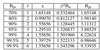
TABLE III
OPTIMAL PARAMETERS FOR THE NON-PERFECT RAINBOW TRADEOFF USED IN PRACTICE.
Rps ` c β2Rtc Rpc
70% 1 1.65148 0.532464 1.65148 80% 2 0.99070 0.812127 1.98140 90% 2 1.55656 1.128445 3.11312 95% 3 1.29510 1.326837 3.88529 99% 4 1.55656 1.501960 6.22624 99.5% 5 1.39729 1.522133 6.98646 99.9% 6 1.55656 1.543296 9.33935
andτFdescribing the times taken for data transfer from disk to main memory and the one-way function computation are also defined as was done previously. Our main claim concerning the optimality of the non-perfect rainbow tradeoff is essentially identical to the perfect case that was given by Theorem 6.
Theorem 12. Let us be given any success rate requirementRps
and any pre-computation table count`. Calculate the matrix stopping constantc= 2{(1−Rps)−2`1 −1}and letRtcbe the tradeoff coefficient calculated through Proposition 11.
The online wall-clock time of the non-perfect rainbow tradeoff that achieves success rate Rps and uses `
pre-computation tables can be minimized to T = 3 223
τ23
Lτ
1 3
FR
1 3
tcN
2 3
withL= 2τF
τL
13R13
tcN
2
3 and F = τL
2τF
23R13
tcN
2 3.
The proof of this theorem is almost identical to that of Theorem 6, except that the relation
c= 2
(1−Rps)−2`1 −1 (26)
is derived from (24). The use of`andcsatisfying this relation guarantees that the probability of success will be Rps.
It only remains to find the optimal value of ` to be used for each probability of success. This part is slightly different from the perfect table case, as there is no bound on c or a corresponding natural extremal value for `. However, since Theorem 12 shows that the minimization of the online time is equivalent to that of the tradeoff coefficient, the minimization can easily be done by substituting a few explicit ` values, together with the corresponding c values given by (26), into the formula forRtcgiven by Proposition 11. Once the optimal
`and the associatedcare found, we gain access to the loaded table entry count L and the computational complexity F. The explicit parameters m and t to be used may then be calculated from the L and F values through Proposition 7 and Proposition 10.
Partial information on the optimal parameters for a number of success rate requirements are listed in Table III, assuming a large s is used. The final column containing the pre-computation coefficient has been calculated withRpc= mt`N =
online time is all we are considering in such a comparison. For example, comparing the numbers for the 99.9% success rate from Table II and Table III, one must consider whether the reduction of the online time in half justifies the five-fold increase in the pre-computation cost.
This completes our analysis and optimization of the non-perfect table rainbow tradeoff algorithm that is used in prac-tice.
REFERENCES
[1] (2013, Jul.) AccessData, Rainbow Tables. [Online]. Available: http:// www.accessdata.com/products/digital-forensics/decryption
[2] (2013, Jul.) Cryptohaze, GPU Rainbow Cracker. [Online]. Avail-able: https://www.cryptohaze.com
[3] (2013, Jul.) Elcomsoft, Advanced Office Password Breaker (Thunder Tables). [Online]. Available: http://www.elcomsoft.com/aopb.html [4] (2013, Jul.) Free Rainbow Tables, Distributed Rainbow Table Project.
[Online]. Available: http://freerainbowtables.com
[5] (2013, Jul,) LastBit, Password Recovery Solutions. [Online]. Avail-able: http://lastbit.com/
[6] (2013, Jul.) Objectif S´ecurit´e, Ophcrack. [Online]. Available: http: //ophcrack.sourceforge.net
[7] (2013, Jul.) Passcovery, Passcovery Suite. [Online]. Available: http:// gpupasswordrecovery.net/news/2012-12-12.htm
[8] (2013, Jul.) Passware, Decryptum. [Online]. Available: http://www. decryptum.com
[9] (2013, Jul.) RainbowCrack Project. [Online]. Available: http:// project-rainbowcrack.com
[10] (2013, Jul.) rcracki mt. [Online]. Available: http://sourceforge.net/ projects/rcracki/
[11] A. Aggarwal and J. S. Vitter, “The input/output complexity of sorting and related problems,” Commun. ACM, vol. 31, pp. 1116–1127, Sep. 1988.
[12] H. R. Amirazizi and M. E. Hellman, “Time-memory-processor trade-offs,”IEEE T. Inf Th, vol. 34(3), pp. 505–512, May 1988.
[13] G. Avoine, P. Junod, and P. Oechslin, “Time-memory trade-offs: false alarm detection using checkpoints,” inProc. Progress in Cryptology (INDOCRYPT 2005), Bangalore, India, Dec. 2005, pp. 183–196. [14] G. Avoine, P. Junod, and P. Oechslin, “Characterization and
improve-ment of time-memory trade-off based on perfect tables,”ACM Trans. Inf. Syst. Secur., vol. 11, Jul. 2008.
[15] E. P. Barkan, “Cryptanalysis of Ciphers and Protocols,” Ph.D. thesis, Technion—Israel Institute of Technology, Mar. 2006.
[16] E. Barkan, E. Biham, and A. Shamir, “Rigorous bounds on cryptanalytic time/memory tradeoffs,” in Proc. Advances in Cryptology (CRYPTO 2006), Santa Barbara, California, USA, Aug. 2006, pp. 1–21. [17] K. Beaver. (2004) A case study in how hackers use windows password
vulnerabilities. [Online]. Available: http://www.dummies.com/how-to/ content/a-case-study-in-how-hackers-use-windows-password-v.html [18] A. Biryukov, A. Shamir, and D. Wagner, “Real time cryptanalysis of
A5/1 on a PC,” inProc. Fast Software Encryption (FSE 2000), New York, NY, USA, Apr. 2000, pp. 1–18.
[19] R. Bragg. (2004) RainbowCrack — Not a new street drug. Redmond Magazine. [Online]. Available: http://redmondmag.com/articles/2004/ 07/01/rainbow-cracknot-a-new-street-drug.aspx
[20] S. A. Cook and R. A. Reckhow, “Time-bounded random access ma-chines,” in Proc. of the 4th Annual ACM Symposium on Theory of Computing (STOC 1972), Denver, Colorado, USA, May 1972, pp. 73– 80.
[21] D. E. Denning, Cryptography and Data Security. Reading, MA: Addison-Wesley, 1982.
[22] T. Guneysu, T. Kasper, M. Novotny, C. Paar, A. Rupp, “Cryptanalysis with COPACOBANA,” IEEE Transactions on Computers, vol. 57, no. 11, pp. 1498–1513, Nov. 2008
[23] M. E. Hellman, “A cryptanalytic time-memory trade-off,”IEEE Trans-actions on Information Theory, vol. 26, pp. 401–406, 1980.
[24] J. Hong, “The cost of false alarms in Hellman and rainbow tradeoffs,”
Des. Codes Cryptography, vol. 57, pp. 293–327, Dec. 2010.
[25] J. Hong and S. Moon, “A comparison of cryptanalytic tradeoff algo-rithms,”J. Cryptology, vol. 26, pp. 559–637, Oct. 2013.
[26] J. Quisquater, F.-X. Standaert, G. Rouvroy, P. David, and J.-D. Legat, “A Cryptanalytic Time-Memory Tradeoff: First FPGA Im-plementation,” in Proc. Field-Programmable Logic and Applications: Reconfigurable Computing Is Going Mainstream (FPL 2002), Montpel-lier, France Sep. 2002, pp. 780–789.
[27] B.-I. Kim and J. Hong, “Analysis of the non-perfect table fuzzy rainbow tradeoff,” inProc. 18th Australasian Conference on Information Security and Privacy (ACISP 2013), Brisbane, Australia, Jul. 2013, pp. 347–362. [28] J. W. Kim, J. Seo, J. Hong, Kunsoo Park, and Sung-Ryul Kim, “High-speed parallel implementations of the rainbow method in a heteroge-neous system,” in Proc. Progress in Cryptology (INDOCRYPT 2012), Kolkata, India, Dec. 2012, pp. 303–316.
[29] K. Kusuda and T. Matsumoto, “Optimization of time-memory trade-off cryptanalysis and its application to DES, FEAL-32, and Skipjack,”
IEICE T Fund, vol. E79-A, pp. 35–48, Jan. 1996.
[30] G. W. Lee, J. Hong, “A comparison of perfect table cryptanalytic tradeoff algorithms,” Cryptology ePrint Archive, Report 2012/540. [Online]. Available: http://eprint.iacr.org/2012/540
[31] R. Lemos. (2003) Cracking windows passwords in seconds. CNET News. [Online]. Available: http://news.cnet.com/2100-1009 3-5053063. html
[32] J. Lyman. (2003) Cracking technique highlights password concerns. TechNewsWorld. [Online]. Available: http://www.technewsworld.com/ story/31178.html
[33] N. Mentens, L. Batina, B. Preneel, and I. Verbauwhede, “Time-memory trade-off attack on FPGA platforms: UNIX password cracking,” inProc. Reconfigurable Computing: Architectures and Applications (ARC 2006), Delft, Netherlands, Mar. 2006, pp. 323–334.
[34] K. Nohl, C. Paget, “GSM-SRSLY?,” presented at26th Chaos Commu-nication Congress (26C3), Berlin, Germany, Dec. 2009.
[35] P. Oechslin, “Making a faster cryptanalytic time-memory trade-off,” in Proc. Advances in Cryptology (CRYPTO 2003), Santa Barbara, California, USA, Aug. 2003, pp. 617–630.
[36] H. Prokop, “Cache-oblivious algorithms,” Master’s thesis, Massachusetts Institute of Technology, Jun. 1999.
[37] F.-X. Standaert, G. Rouvroy, J.-J. Quisquater, and J.-D. Legat, “A time-memory tradeoff using distinguished points: new analysis & FPGA results,” in Proc. Cryptographic Hardware and Embedded Systems (CHES 2002), Redwood Shores, CA, USA, Aug. 2002, pp. 593–609. [38] Kostas Theocharoulis, Ioannis Papaefstathiou, Charalampos Manifavas,
“Implementing rainbow tables in high-end FPGAs for super-fast pass-word cracking,” in Proc. International Conference on Field Pro-grammable Logic and Applications, Milano, Italy, Aug. 2010, pp. 145– 150.