Low complexity DOA estimation from short data snapshots for ULA systems using the annihilating filter technique

R E S E A R C H

Open Access

Low-complexity DOA estimation from

short data snapshots for ULA systems using

the annihilating filter technique

Faouzi Bellili

, Souheib Ben Amor

, Sofiène Affes

and Ali Ghrayeb

Abstract

This paper addresses the problem of DOA estimation using uniform linear array (ULA) antenna configurations. We propose a new low-cost method of multiple DOA estimation from very short data snapshots. The new estimator is based on theannihilating filter(AF) technique. It is non-data-aided (NDA) and does not impinge therefore on the whole throughput of the system. The noise components are assumed temporally and spatially white across the receiving antenna elements. The transmitted signals are also temporally and spatially white across the transmitting sources. The new method is compared in performance to the Cramér-Rao lower bound (CRLB), the root-MUSIC algorithm, the deterministic maximum likelihood estimator and another Bayesian method developed precisely for the single snapshot case. Simulations show that the new estimator performs well over a wide SNR range. Prominently, the main advantage of the new AF-based method is that it succeeds in accurately estimating the DOAs from short data snapshots and even from a single snapshot outperforming by far the state-of-the-art techniques both in DOA estimation accuracy and computational cost.

Keywords: DOA estimation, Root-MUSIC, Annihilating filter, Array signal processing, NDA estimation

1 Introduction

In recent years, there has been a surge of interest in array signal processing applications in both military and civil domains [1, 2]. The concept of direction of arrival (DOA) estimation find its use in applications related to radar or sonar systems. In addition, in modern mobile communication systems, for example, based only on the data received at the antenna array, estimating the DOAs of the desired users and those of the interference signals allows their extraction and cancellation, respectively, by beamforming technologies [3, 4] in order to improve the wireless systems’ performance.

Roughly speaking, depending on the a priori knowledge of the transmitted signals, DOA estimators can be cate-gorized as data-aided (DA) or non-data-aided (NDA). In plain English, DA approaches base the estimation pro-cess on a priori perfectly known symbols. Unfortunately, although being simple and accurate, these approaches may

*Correspondence: [email protected]

1_{INRS-EMT, 800, de la Gauchetière Ouest, Suite 6900, H5A 1K6 Montréal, QC,} Canada

Full list of author information is available at the end of the article

suffer from the major drawback of limiting the whole throughput of the system by periodically sending a ref-erence (known) signal [5]. It should be mentioned here that superimposed pilots do not affect the throughput but increase the complexity of the channel estimation process. Hence, the ever increasing demand for channel bandwidth spurred the more practically oriented minds to develop new estimation techniques that rely on the received data samples only and which are therefore commonly known as NDA techniques. NDA estimators themselves are referred to as deterministic or stochastic if the unknown transmit-ted signal is assumed deterministic or completely random, respectively. So far, from maximum likelihood-based to subspace-based methods, many NDA DOA estimators have been proposed and extensively studied in the litera-ture [6–8]. The NDA maximum likelihood approaches are undoubtedly the most accurate, but unfortunately, they are often computationally very expensive. To circumvent this challenging problem, covariance-based estimators are often a trend—in NDA estimation schemes—to alleviate this burden of computational cost. Fortunately, usually,

they also provide sufficiently accurate DOA estimates, especially in the presence of sufficiently large number of received samples. But in situations of short data snap-shots, they may not be reliable and one would be obliged to trade low complexity for more accurate estimation by simply applying the maximum likelihood approaches. Yet, the maximum likelihood estimators are analytically intractable in the NDA case especially in the presence of random transmitted symbols/signals. Therefore, they are often tackled numerically via multidimensional grid search approaches. Their accuracy/resolution is therefore dictated by the discretization step of the grid. A very dense discretization (small step) is able to provide very accurate estimates even at low operational SNRs, but the complexity of the underlying ML algorithm would be extremely high and even prohibitive since its complexity grows exponentially with the number of the parameters to be estimated. Another alternative is to solve the ML cri-terion using pilot/reference symbols/signals only where a closed-form solution may be feasible. Unfortunately, this approach is not able to providein-serviceestimates as the receiver is compelled to wait for the next pilot signals in order to update the estimates.

Motivated by these facts, we develop in this paper a new covariance-based DOA estimation method for ULA con-figurations which succeeds in estimating the DOA from very short data records. It is based on theannihilating fil-ter technique: finding the roots of an annihilating filter (AF) which are directly related to the unknown DOAs. It should be noted that the AF technique has been well known for a very long time in the mature field of spectral estimation. About a decade ago, it was also used to suc-cessfully develop the so-called finite-rate-of-innovation (FRI) sampling method [9] where it led to signal sampling and reconstruction paradigms at the minimal possible rate (far below the traditional Nyquist rate). In this contribu-tion, we apply for the first time the AF approach to DOA estimation for ULA configurations and, therefore, we will henceforth refer to our new technique as the AF-based method. The coefficients of the corresponding AF are cal-culated by the singular value decomposition (SVD) of a matrix whose elements are built from second-order cross moments across the receiving antenna elements of the received samples. Interestingly, this matrix is of reduced dimensions thereby yielding a very low computational load of the SVD decomposition.

We propose two different versions of the new AF-based solution1depending on the SNR threshold. The first one, referred to as “version I”, is more advantageous at high SNR levels. It exploits each consecutive 2K + 1 corre-lation coefficients along the columns and rows of the covariance matrix (K being the number of sources). The second one, referred to as “version II”, exploits the Toepltiz structure of the covariance matrix in order to enhance

the estimation performance at low SNR levels. In both versions, the obtained DOA estimates are then used to find the unknown sources’ powers along with the noise variance.

In the multiple snapshot case, both versions of the proposed AF-based technique are compared in accuracy performance to the Cramér-Rao lower bound (CRLB) [10] and to the root-MUSIC algorithm—a popular and pow-erful technique of DOA estimation for ULA systems— which is also based on polynomial rooting [11]. In the single-snapshot scenario, however, it is compared to another Bayesian method that was designed precisely for the challenging single-snapshot case [12] as well as the deterministic ML (DML) estimator. We mention here that a more recentiterativetechnique that handles the single-snapshot case has also been proposed in [13]. Unfortu-nately, in its NDA version, it relies on the prior avail-ability of an initial guess about all the unknown DOAs whose accuracy affects the overall performance of the method. Therefore, for the sake of fairness, this technique is not considered since none of the considered techniques (including our AF-based estimator itself ) requires an ini-tial guess about the DOAs. Even more, it has been recently recognized in a comparative study of various DOA esti-mators [14] that DML is indeed the most attractive one if the DOAs are to be estimated from a single snapshot. It will be shown by Monte-Carlo simulations that the new AF-based method is able to accurately estimate the DOAs from short data snapshots and even from a single-shot measurement. Furthermore, it outperforms the classical Bayesian and DML estimators over a wide SNR range with a slight performance advantage for the latter in the low SNR region but at the cost of an extremely high computational load.

We organize the rest of this paper as follows. In Section 2, we introduce the system model that will be used throughout this article. Then in Section 3, we develop our new AF-based DOA estimation technique. In Section 4, we exploit these new AF-based DOA estimates to develop new estimates for the channel powers. In Section 5, we assess the performance of the new estimators. Finally, we draw out some concluding remarks in Section 6.

2 System model

We consider a uniform linear array (ULA) ofNaantenna elements immersed in a homogeneous media in the far field ofKpoint sources that are transmitting multiple pla-nar waves. We assume that the transmitted signals are temporally white and uncorrelated between the radiating sources. Assuming perfect frequency synchronization, the received signal on the{ith}Na

i=1antenna element, at the out-put of the matched filter, can be modelled as a complex signal as follows: ponent on the ith antenna branch that is modelled by a zero-mean complex Gaussian random variable with inde-pendent real and imaginary parts, each of variance σ2. The complex channel coefficients corresponding to theK sources are assumed to be unknown, and they are denoted by {hk = |hk|ejφk}K_k=1 where φk stands for any possi-ble channel distortion phase. Moreover,{θk}K_k=1 are the unknown DOAs (to be estimated) of the planar waves impinging from theKsources.

Note here that the receiving antenna elements are sup-posed to be spaced by half the wavelength, i.e. d =

λ/2 where d is the distance between two consecutive antenna branches andλis the carrier wavelength of the signal. Note also that although the vector/matrix repre-sentation of the received signals is more compact and widely adopted in the open literature, we settle here on the scalar form of the received signals (i.e. the elemen-tary received signals on each antenna element). We believe that this representation allows for an easy grasp of the theoretical foundations of the new estimator since it is— as will be seen later—based on the explicit expression for each cross-covariance between the elementary received signals.

We assume hereafter that at each time instant n the transmitted signals,a(n) =[a1(n), a2(n),· · ·, aK(n)]T and the noise componentsw(n)=[w1(n),· · ·, wNa(n)]T

are each uncorrelated element-wise, i.e.

E{w(n)Hw(n)} =2σ2INaandE{a(n)Ha(n)} =IK, (2)

where in the last equality, we assume, without loss of generality, that the energy of the transmitted signals are normalized to one, i.e.E{|ak(n)|2} =1. In fact, the trans-mitted powers, Pk = E{|ak(n)|2}, can always be incor-porated in the channel coefficients after being scaled by the factor√P_k. Finally, the symbols,{a_k(n)}N_n=1, transmit-ted by source k over the observation time window are assumed mutually independent. Then, we define the true SNR of thekthsource as follows:

ρk

E{|hk|2|ak(n)|2}

2σ2 =

|hk|2

2σ2. (3)

3 Formulation of the new AF-based DOA

estimator

In few words, we mention that the new AF-based estima-tor relies on a special property that is inherent to appropri-ately selected sequences of second-order cross-moments of the received signals. Therefore, we will simply begin by deriving the explicit expression of the elementary cross-covariances between the different antenna branches. To that end, and by assuming a perfect knowledge of the number of signalsK, we gather for more convenience all the unknown DOAs in one single parameter vectorθ = [θ1, θ2,· · ·, θK]T. Then, the cross-covariances between the received signals from any pair(i,l) of the receiving antenna array can be defined as:

y(i,l) E{yi(n)yl∗(n)}, i,l=1, 2,· · ·,Na. (4) Recall the fact that the transmitted signals and the noise components are spatially and temporally white; hence, Mθ(i,l)reduces simply to:

be easily computed together using the vector/matrix rep-resentation of the received signals. Indeed, denoting by

y(n)=[y1(n), y2(n),· · ·, yNa(n)]

T_{, (6)}

the received vector at time instant n, y(i,l), is noth-ing but the (i,l)thentry of the covariance matrix, y =

E{y(n)yH(n)}. The latter matrix is Toeplitz structured3 due to the use of an ULA antenna and can be estimated by a simple sample mean as follows:

We mention here that sincey

andy

is a Hermitian matrix (i.e. y = Hy), then the strictly lower

triangu-lar matrix obtained fromycontains all the information

about the DOAs that would be extracted from the entire matrix. Indeed, the diagonal elements do not depend on the unknown DOAs, although they can be eventually used to estimate the noise variance after estimating the chan-nel coefficients from the off-diagonal entries as detailed later. Consequently, from now on, the counters i and l will always verify4i > l. Then, using the notationuk = ejπsin(θk)_{, we define the N}

a − 1 sequences—indexed by the counterl—{r_θ(l)[m]}Na−l

r(_θl)[m] = y(l+m,l), m=1, 2,· · ·,Na−l, (8)

which is simply given by

r_θ(l)[m] = dimensional vectorr(_θl)—that will be used subsequently— as follows5: is simply a weighted sum of exponentials. This interesting property is very useful—when combined with the anni-hilating filter technique—and is actually the main idea behind this work as will be soon explained.

Generally speaking, a filter g[m] is called an annihilat-ing filter of a signal or more generally a discrete sequence

{s[m]}mwhen

(g∗s)[m]=0, ∀m ∈Z, (11) where ∗ stands for the discrete convolution. Usually, the filtering operation is applied to signals. But in this paper, we filter a sequence of cross-covariances by inter-preting them as received samples. Therefore, the

cross-covariances sequence r(_θl)[m]Na−l

m=1 will play the role (interpreted as) of the signal sequence s[m] in (11). Indeed, as shown subsequently, for such special sequences (linear combinations of exponentials), the roots of the corresponding annihilating filters are exactly the involved elementary exponentials. More formally, consider the fol-lowing filter:

Therefore, g[n]—as constructed in (12)—is indeed an

annihilating filter for the sequencer(_θl)[m]Na−1 m=1. Then, if one is able to find the coefficients{g[n]}K_n=0, the roots of the corresponding polynomial g(z) in (12) would be easily computed and then the DOAs can be easily esti-mated from the arguments of the obtained roots. To that end, we gather the desired coefficients, {g[n]}K_n=0, in a single unknown vectorg= g[ 0] ,g[ 2] ,· · ·,g[K]T and describe below an easy SVD procedure that enables find-ingg.

First notice that the unknown filter coefficients{g[n]}K_n=0 ing(z)=_nK₌₀g[n]z−nmust be such that (11) is satisfied the lthcolumn of the covariance matrix, we estimate (as described later) from (14) theK+1 unknown filter coef-ficients. In this way, it is clear that one needsK+1 inde-pendent equations—obtained by changingm—in order to obtain at least one estimate,gˆ(l), of the desired vectorg. Therefore, if a columnlis to be useful, the corresponding vectorr(_θl)should contain at least 2K+1 elements. Recall from (10) that the size ofr(_θl) isNa−l, which results in Na−l≥2K+1. Therefore,lmust verify

1≤l≤Na−2K−1, (15)

meaning that only the firstNa−2K −1 columns of the covariance matrix contain a sufficient number of cross-covariances that enable having at least one estimate,gˆ(l)

ofg, per-column ing antenna elements forK unknown sources. Thus, our estimator needs more than twice the number of antennas as the number of sources. Moreover, in addition to the trivial initial estimate,g(₀l), that is obtained using the first necessary 2K+1 cross-covariances inr(_θl), we can actually obtainPladditional estimates

ˆ

g(_pl)Pl

p=1for the unknown

K

n=0

g[n]r(_θl)[mp+r−n]=0,r= −K,−K+1,· · ·,K−1,K. (16)

Therefore, for each value ofp(or equivalentlymp), we have K + 1 independent equations which can be more conveniently written in the matrix/vector form as follows:

S(_pl)(θ)g=0, (17) linear systems (by varyingp) that provideP_l+1 estimates for the same vectorg—involved in these systems—as pre-viously stated.

In practice, the system in (17) can be solved via a singu-lar value decomposition (SVD) where the(K+1×K+1) unknown DOAs are obtained for eachlandpas follows:

ˆ where ∠(.) returns the angle of any complex number. Finally, recall that for the{lth}Na−2k−1

l=1 column, we have P_l +1 = Na−2K −lestimates for the same DOAθk, which means that by considering all the eligible columns, we have

estimates for each DOA. Therefore, one can average over all these estimates (obtained column wise) to obtain more refined estimates for the unknown DOAs as follows:

ˆ exploited to further refine the DOA estimates. This may seem a priori impossible since these columns—or

equiv-alently the corresponding vectors indeed contain the necessary 2K+1 cross-covariances as previously required. Yet, the elements of these columns belong to the last Na −2K −1 rows that contain nec-essarily more than 2K +1 adjacent covariances. Indeed, recalling that the covariance matrix¯(y)is Toeplitz struc-tured, it becomes clear that the lastNa−2K− 1 rows can also be exploited in the same way providing thereby a new set of estimates for the DOAs. To that end, for the{lth}Na

l=2K+2row, we construct the corresponding

vec-tors6_,r(l) of linear combinations of weighted exponentials. Then, applying the same procedure using the vectorsr_θ(l)instead ofr(_θl), we obtain an additionalrow-wiserefined estimate for each DOA which we denote θˆ_krow. Lastly, the final estimates of the DOAs are obtained as

ˆ Based on the analysis so far introduced, it may seem that the new estimator works only if an extremely large num-ber of snapshots are available at the receiver side. In fact, all the derivations are based on the theoretical expression of the elementary cross-covariances,y(i,l), given in (5)

although in practice these elementary cross-covariances are estimated by sample averaging as follows:

3.1 Robustness to the presence of short data records The resilience to the presence of short data records can be proven theoretically. In this analysis, we considers the case of short data records but it is also valid for the single-snapshot scenario by simply takingN =1. For con-venience, we adopt the notationl_y(i) for the estimated elementary cross-covariances of (25) instead of y(i,l),

which are given by

and we show that the unknown DOAs can still be esti-mated from the roots of the corresponding annihilating filter. In fact, we have forn=1, 2,· · ·,N: Then, for medium and high SNR values, the noise com-ponents are small compared to the useful signal compo-nent, i.e.|wi(n)| |Kk=1hkak(n)ej(i−1)πsin(θk)|with very Therefore, the second term in (27) (stemming from the noise component) can be reasonably neglected, and we obtain an approximate expression for the estimated covariances between antenna elementiand antenna ele-mentl, as follows:

We observe from (29) that the second-order moments estimated with short data records (or even a single snap-shot) exhibit the interesting property of a “weighted sum of sinusoids” and therefore the DOAs can still be accu-rately estimated from the roots of their annihilating filter.

3.2 Exploiting the Toeplitz structure of the covariance matrix

When the propagation conditions are very harsh, the SNR experienced at the receiver side can be very low. In this scenario, the received signals are too much corrupted by the noise components and therefore the estimated cross-covariances are very noisy, especially from short data records. Hence, exploiting the fact that the covari-ance matrix is Toeplitz structured, one can average along the secondary diagonals in order to obtain a set of more accurate estimates for the cross-covariances. The DOA estimation is then performed in the same way using the new single sequence of more accurateNacovariances. In fact, we see from (5) that form=1, 2,· · ·,Na−1

y(l+m,l) = y(1+m, 1), l=1, 2,· · ·,Na−m. (30) Therefore, for each fixed lag m, {y(l + m,l)}N_l=a₁−m

can be averaged as follows to obtain the following more refined statistics: that was previously applied for all the eligible columns is now applied to the single vectorr¯θ since it also inherits the interesting property of weighted sum of exponentials. For ease of notation, we simply refer to this procedure asversion IIof the new AF-based estimator and we refer to the procedure described previously (column-wise and row-wise) asversion I.

whole information is being exploited. Therefore, as long as the SNR decreases or the number of sources increases (for a fixed number of receiving antenna elements), it is expected that the second version of the new estimator out-performs its first version. However, for sufficiently high SNR values, the estimated elementary cross-covariances (without averaging) are already quite accurate and can hence be reliably used to obtain more accurate7 DOA estimates withversion I. The latter is even more recom-mended if the number of sources is also small since the number of eligible columns (and consequently the num-ber of exploited cross-covariances) would be sufficiently high.

3.3 Complexity analysis

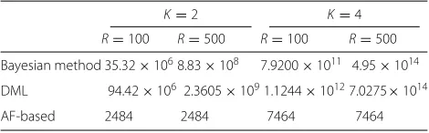
In this subsection, we assess the complexity of the new estimator vs. the other single-snapshot techniques8. To that end, we evaluate the number of operations (addi-tions and multiplica(addi-tions) required by each estimator. In particular, the new estimator involves two major steps which are (i) the estimation of the covariance matrix that requires NNa(Na − 1) operations and (ii) the SVD decomposition and polynomial rooting proce-dures which require 2(Na − 2K − 1)(Na − 2K)O(K3) operations. Of course, it involves also at the very end a simple step in which the individual estimates are averaged requiring (Na − 2K − 1)(Na − 2K) extra operations. On the other hand, the overall com-plexities of the DML and Bayesian estimators are RK2N_a3+(N+2K−1)N_a2+(4Na−1)K2−(N+Na)

K+O(K3) and RK(4K+3)N_a2+(12Na−3)K2−

(3K−2)Na+3O(K3)

, respectively, where R is the number of samples on the parameters grid corresponding to a discretization step, s, of s = 180/R. Notice here that the complexity of these two traditional estimators grows exponentially with the number of unknown DOAs, K, as reflected by the multiplicative term RK. It comes clear now that increasingR(i.e. considering a denser grid search for more refined estimates) increases prohibitively their computational cost. Typically, forNa = 16,Ns= 2, N = 1, and R = 100, the total number of operations performed by our AF-based method, to estimate all the DOAs, is about 2484 operations. However, to evaluate their objective functions just at a single search point (θi,θj) in the grid, the Bayesian and DML estimators require about 3532 and 9442 operations, respectively, i.e. already far more than the overall complexity of our estimator. To find the estimates of the DOAs as the maxi-mum of their objective functions over all the grid points, these two classical estimators require in total as much as 1002×3532=35.32×106and 1002×9442=94.42×106 operations against just 2484 operations with the proposed estimator. Of course, the performance of these grid-search estimators improves constantly as R increases,

but their computational load becomes prohibitively very high. This is illustrated in Table 1 where we present the computational load of the three estimators in different setups by evaluating their complexities at various values for the couple(K,R)with a fixed array-size ofNa = 16. It is clearly seen from this table that our estimator is far less computationally expensive than both existing single-snapshot techniques. Moreover, it will be shown later through computer simulations that it outperforms both of them in accuracy over a large SNR range.

4 Per-source channel power estimation

The per-source estimation of the channel power (or signal power) is very useful in wireless communication systems. In fact, in a multi-user mobile communication system— where each active user can be seen as an active source— the knowledge of this parameter is used to manage the interference. For instance, a well-known scheme for multi-user detection is the successive interference cancellation (SIC). The scheme is based on demodulating the strongest interferer and removing its effect from the received sig-nal [15] and then continuing this procedure for the next strongest user. Because of its simplicity and also its capa-bility in combating strong interferers [15], SIC is the subject of great attention for practical systems design; see [16–18] and references therein. Clearly, SIC requires the power of the strongest interferer at each stage of inter-ferer cancellation. There are of course many other useful applications beyond this example that justify the need of properly estimating both the source and noise powers and the SNR. Motivated by this fact, we exploit the DOA estimates provided by our AF-based technique in order to estimate the individual channel powers almost instan-taneously over a very short data records (N < 10 for instance). To that end, we take the firstKaveraged covari-ances in (31),r¯θ[m]= K_k=1|h(k)|2um_k,m = 1, 2,· · ·,K, from which we write the following matrix system:

⎛

Table 1Complexity of the three single-shot techniques with

Na=16 receiving antenna branches

K=2 K=4

R=100 R=500 R=100 R=500 Bayesian method 35.32×106_8.83×108 _7.9200×1011 _4.95×1014

DML 94.42×106 _2.3605×109_1.1244×1012_7.0275×1014

Now injecting the estimated DOAs, θk, in uk instead of the true DOAs,θk, we construct an estimated matrix,

U(θ), using uk = ejπsin(θk), to substitute U(θ) in the system (32) in which the only remaining unknowns are

{|hk|2}K_k=1. Thus, by invertingU(θ)and usingr¯θ instead of r¯θ, one can easily obtain a joint estimate, h =

[|h1|2,|h2|2,· · ·,|hK|2]T, for the channel powers, h = [|h1|2,|h2|2,· · ·,|hK|2]T, as follows:

h = U(θ)−1r¯θ. (33) Note thatU(θ)is a Vandermonde matrix and therefore its inverse always exists as far as the DOAs are different (resolvable DOAs). Now after obtaining the estimates of

{|hk|2}K_k=1, we extract an estimate of the noise power from the main diagonal elements of the covariance matrix. In fact, we see from (5) that for the{lth}Na

l=1diagonal element, we have which can be averaged over all the possible values oflto obtain a more accurate estimate of the noise variance:

" Finally, using (33) and (36), an estimate of the SNR of each source is simply given by

ρk = |

_hk|2

2σ2. (37)

5 Simulation results

In this section, we assess the performance of the new DOA estimator using the mean square error (MSE) as a perfor-mance measure. The MSE is computed for each estimator

ˆ where Mc is the number of Monte-Carlo simulations which is set to Mc = 1000 in all simulations and θˆ_k(q) is the estimate of θk from theqth Monte-Carlo run. We also consider the well-known root-MUSIC (RM) estima-tor and the Cramér-Rao lower bound (CRLB) [10] as a benchmark against which we compare the performance of our newly developed method in the case of a large number of snapshots. In the case of short data records,

we also add the Multi-Task Bayesian Compressed Sensing (MT-BCS) technique [19] as a benchmark. We propose also another performance metric where we show the res-olution probabilities for the AF-based and root MUSIC techniques. In the more challenging case where a sin-gle snapshot is available at the receiver side, we compare our method to the Bayesian estimator [12] and the Single Task Bayesian Compressed Sensing (ST-BCS) technique [19] that are both specifically designed to cope with this extreme scenario. We also compare it to the deterministic ML estimator that is recognized to be the most accurate in this case [14]. For the sake of conciseness, we consider without loss of generality the case of equipowered sources and provide simulation results only for the first source (DOA and channel power). Yet, we emphasize the fact that the same performance behaviour can be observed from the other sources. For the channel power estimator, we adopt the normalized root mean square error (NRMSE) as a performance measure defined as

NRMSE(|hk|2) =

The NRMSE for the SNR estimator is defined like-wise. DOA estimation will be basically organized in three subsections: (i) the case of multiple snapshots (including short-data records), (ii) the case of a single-shot measure-ment, and (iii) the case of time varying DOAs. Channel powers and SNR estimation will then follow.

5.1 Multiple and short-data records: comparison against

root-MUSIC

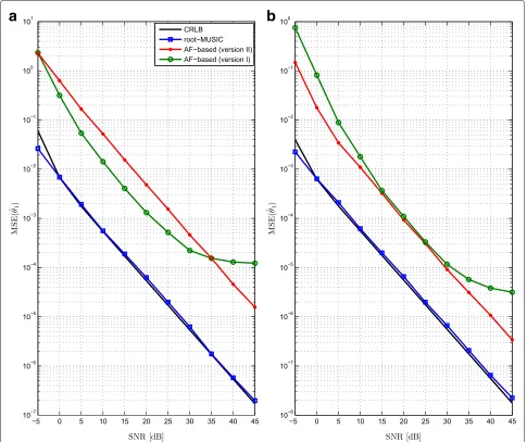
In Fig. 1, we plot for the three estimators (version Iand verion II of the AF-based and root-MUSIC) the MSE of the DOA estimates for the first source obtained from N = 1000 received samples, withNa = 8 andNa = 16 receiving antenna elements, versus the SNR of the same source.

a

b

Fig. 1MSE for the first DOA versus the SNR withK=2 sources,N=1000 snapshots,θ1=18°, andθ2=36°: (a)Na=8 antenna elements and (b) Na=16 antenna elements

by applying version II. The same observation holds for sufficiently high SNR values even ifNais small (Na=8).

In Fig. 2, we simulate a more adverse situation in which the DOAs are estimated from a very limited number of snapshots (N = 3 for example). The major advantage of our new estimator is now revealed. In fact, both ver-sions of the new technique outperform by far, in terms of estimation accuracy, the RM estimator with an advantage forversion IIoverversion I (the advantage of exploiting the Toeplitz structure is now clearer). Yet, the former’s performance saturates at very high SNR values whereas the latter’s improves linearly with the SNR. The MT-BCS technique shows in Fig. 2 good performance in the case of short data records (i.e.N=3). Unfortunately, its compu-tational complexity is dictated by the grid discretization

step, and a trade-off between complexity and performance must be made.[19].

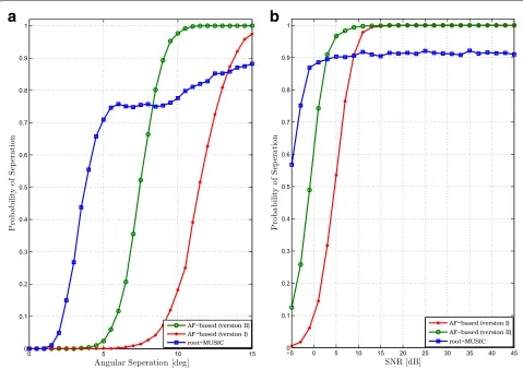
In Fig. 3, we provide the probability of separation ver-sus the angular separation and the SNR. The probability of separation, as defined in [20], states that two signals are said to be resolved if their respective DOA estimates,

ˆ

θ1 and θˆ2, are such that | ˆθ1 − θ1| < |θ1 − θ2|/2 and

Fig. 2MSE for the first DOA versus the SNR withK₌2 sources,N₌3 snapshots,_θ1=18°,θ2=36°, andNa=8 antenna elements

techniques succeed in resolving the sources in 90% of the cases starting from the SNR value of 3 dB.

5.2 Single-shot case: comparison against the DML and

Bayesian methods

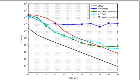
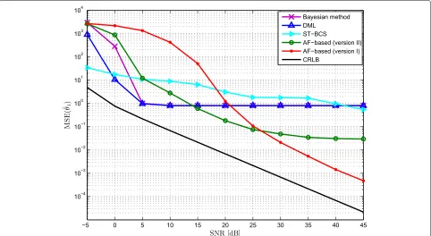
Now, we consider a situation which is even more challeng-ing where we assume that the receiver needs to estimate the DOAs from a single snapshot. In this situation, we compare the performance of our method against that of three estimators that are tailored specifically to the single-shot case: the Bayesian method of [12], the single-single-shot DML estimator [14], and ST-BCS. We recall that, accord-ing to the recent survey of [14], the DML technique stands as the most accurate among various single-shot estima-tors. We plot in Fig. 4 the MSE for the four estimators for N=1 (i.e. only one sample is available at the receiver side) andNa=16 receiving antenna branches.

The three existing estimators were simulated using a discretization steps = 180/100 (in the remainder of this paper, we will characterize the grid step,s, by the integer numberRwheres=180/R). We observe from this figure that both versions of the newly developed AF-based esti-mator are still able to estimate the DOAs over a wide SNR range.

We see also from Fig. 4 that for sufficiently high SNR values the MSE ofversion IIsaturates, contrarily to ver-sion I. This is because in this SNR region the signals

are almost noise-free and therefore the elementary cross-covariances’ estimates are already noiseless. They can be thus exploited as they are (as done in version I) to pro-vide a large number of sufficiently accurate estimates

ˆ

θ(l,p)

k withoutprior averaging (as done in version II). In fact, averaging along the secondary diagonals would sim-ply provide a number of statistics that are as accurate as the elementary cross-covariances themselves, and hence, the performance in terms of DOA estimation does not improve (saturation).

On the other hand, the existing single-shot techniques (Bayesian, DML estimators and ST-BCS) exhibit a slight advantage at low SNR levels, but their computational load is extremely much higher. In fact, in light of the complex-ity analysis presented in Table 1 at the end of Section 3.3, the complexities of the DML and Bayesian algorithms are, respectively, in the order ofNoperBayesian = 35.32×106and N_operDML=94.42×106operations against onlyN_operAF =2484 operations for the proposed estimator. This amounts to

complexity ratios in the order of N

Bayesian

oper

NoperAF ≈

NDML

oper

NoperAF ≈ 10

4_.

a

b

Fig. 3Probability of resolution (a) versus angular separation (N=3 andSNR=15 dB) and (b) versus SNR ( θ=15°andN=3)

range, but unfortunately their complexities become even more prohibitive9. For example, under the same simula-tion setup of Fig. 4 (in particularNa = 16 andK = 2), these two estimators will outperform the AF-based tech-nique, over the entire SNR range, by setting R = 500 (i.e. estimating the DOAs at a grid resolution of 0.36°). However, the complexity ratios become in the order of

NoperBayesian

NoperAF ≈

NoperDML

NoperAF ≈10

6_.

The new method is therefore very useful (in terms of accuracy/complexity trade-offs) in applications where a single snapshot is to be used. This is encountered in many situations where a very high estimation update speed is required. These applications can be indeed enhanced by providing a DOA estimate once a sin-gle sample is acquired instead of waiting for a larger number of measurements. Furthermore, in many other practical situations, the DOAs may change apprecia-bly from one snapshot to another due to the fast motion of the sources. For all these systems, our new AF-based estimator offers the best accuracy/complexity trade-offs.

5.3 Time-varying DOAs

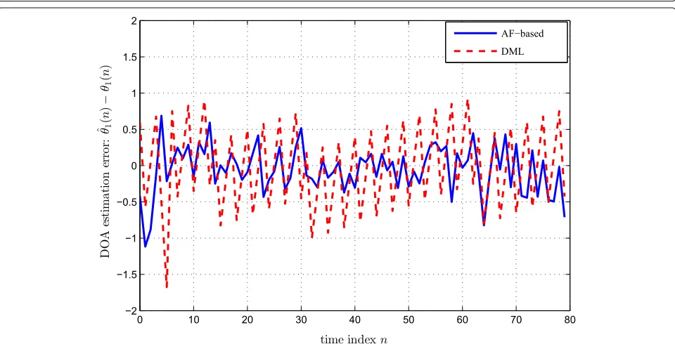
To illustrate the time-varying DOA tracking capability of the new AF-based estimator, we plot in Fig. 5 the esti-mated DOAs using itsversion IIand the DML algorithm for two moving sources and an SNR level of 15 dB . The DOAs were generated assuming that both sources increase linearly from−60° and−30°, respectively, with a radial speedθ˙1 = ˙θ2as high as 1.175° per sample, over 80 data snapshots. Both estimators were applied using N = 1 (i.e. single snapshot). It is seen that both AF and DML estimates follow accurately the trajectories of the two time-varying DOAs. Yet, as depicted in Fig. 6, the AF-based estimator exhibits lower tracking error at significantly much less computational cost. Furthermore, since the new estimator performs well with a single data snapshot, its tracking performance will prove the same no matter the angular speed ranges of the DOA time variations reach.

Fig. 4MSE for the first DOA versus the SNR withK₌2 sources,N₌1,_θ1=20.7°,θ2=40.5°,Na=16 antenna elements, and 16−QAM

on the angular speed range, the AF-based estimator might outperform root-MUSIC even when data records are not short. In fact, when the DOAs are not constant over a time period, applying the root-MUSIC algorithm locally— over an observation window of short size—would simply return an estimate of the average DOAs over this consid-ered window. Clearly, in this case, the performance of the root-MUSIC algorithm is affected by the size of the local window and the DOAs speed. Indeed, as speed increases, the DOAs tend to vary appreciably within the process-ing window duration and, hence, the performance of the root-MUSIC estimator degrades as the approximation of locally constant DOAs becomes increasingly inaccurate. Our new estimator, however, does not suffer from this drawback since it succeeds in accurately estimating the DOAs from very short data records and since it is also very robust to fast DOA time variations (as seen from Figs. 2 and 5). This behaviour is illustrated in Fig. 7 where we show the operational regions, in terms of window sizes (N) and DOA speeds (θ˙), for the two estimators. A region is attributed to a given estimator when this estimator shows lower MSE for all the couples (N,θ˙) in this region. We see that when the DOAs vary so rapidly, our new esti-mator outperforms the RM technique even in the case of multiple snapshots (upper right corner of Fig. 7) contrar-ily to what was observed in Fig. 1 where the DOAs where assumed constant (which corresponds toθ˙ = 0°/sample andN=1000).

5.4 Performance of the channel powers and SNR

estimators

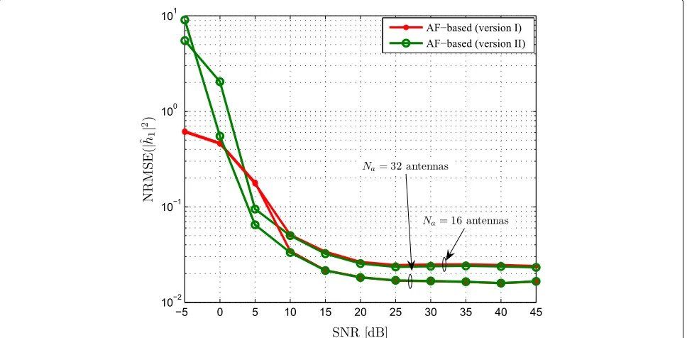
Here, we assess the performance of the channel power estimator derived in section IV. For two different values of the observation window sizes, namely N = 10 and N = 1000, we plot in Figs. 8 and 9, respectively, the NRMSE for the channel power estimator using both ver-sions I andIIas a function of the true SNR. First, notice from Fig. 8 that the channel power is estimated quite accu-rately using only few received samples,N =10 snapshots, especially in the moderate/high experienced SNR values. Naturally, the estimation accuracy is enhanced in Fig. 9 for a larger window size, i.e.N = 1000 where both versions provide very accurate estimates for the channel power, a key parameter that is often used for the design of wire-less communication schemes. We also observe from these two figures, for these large antenna array-sizes (Na = 16 andNa = 32), the performance improvements ofversion Iagainstversion IIat low SNR values, a fact that is mainly due to the improvements in DOA estimation in this region as explained previously (see comments on Fig. 1).

a

b

Fig. 5True DOAs and their estimates with QPSK,K₌2 sources,N₌1,_θ˙1= ˙θ2=1.175°/sample,R=100,Na=16 and SNR=15 dB: (a) AF-based

(version II) and (b) DML

Fig. 7Operational regions for the AF-based (white surface) and the root-MUSIC (black surface) estimators withK=2,Na=8, and SNR=25 dB

argue that since the channel strengths are increasingly more accurate at higher SNR values, then the estima-tion error on the noise power should also remain con-stant and so does the SNR estimates. This is simply not true because as the true SNR increases, the true channel strength increases as well (for a fixed true noise vari-ance) and the relative estimation errork = |ˆhk|2− |hk|2 is higher although the normalized error ˜k = k/|hk|2

remains constant in average (i.e. the channel estimates’ NRMSE remains constant). Consequently, larger{k}K_k=1 yields a higher estimation error on the noise power (or equivalently the SNR); k can be even larger than 2σ2 to be estimated itself. For a larger number of receiving antenna elements (Na = 32 for example), the SNR esti-mates are, however, reliable for the entire considered SNR region.

Fig. 9NRMSE of the channel power estimators (versions IandII) withN₌1000,_θ1=18°,θ2=36°,K=2,Na=16, 32, andσ2=2

6 Conclusions

In this paper, we derived a new DOA estimation method for multiple planar waves impinging on a ULA antenna array. The transmitted sources and the noise components are assumed to be spatially and temporally white. The new method is based on theannihilating filter technique. It

was seen that the new method exhibits accurate statisti-cal performance while having a low computational cost. Its major advantage is its capability of accurately resolving DOAs as close as 10°from short data snapshots and even from a single snapshot. This capability makes this new estimator well geared toward applications that require

DOA estimation of fast moving sources or require up-to-date estimates for the DOAs over very short observation windows. The estimated DOAs were then used to easily estimate the channel powers and SNRs for each source (or user).

Endnotes

1_{Extensions of the proposed AF-based technique to the}

problem of joint angle and delay estimation (JADE) [21] falls beyond the scope of this paper.

2_{The signala}

k(n)can be complex symbols taken from any constellation such as QPSK, M-PSK and M-QAM or simply complex Gaussian.

3_{This is because all the cross-covariances that belong}

to any given secondary diagonal of the covariance matrix have the same expression.

4_{One could decide to consider the upper-triangular}

matrix, i.e.i < l. But this does not change the estimator, as seen from (5), since this will only introduce a negative sign in the exponential argument.

5_{Note that the vectorr}(l)

θ contains all theNa−lelements of thelthcolumn that are lying under the main diagonal of the covariance matrix.

6_{We mention here that r}(l)

θ plays the role of r(θl) that was previously used when the estimation process was performed column-wise.

7_{This is because this version provides a larger}

num-ber of estimates for each DOA, which can be averaged to obtain a more refined final estimate.

8_{Please note that the root-MUSIC techniques has}

almost the same complexity of the our AF-based estima-tor since it involves similar operations of SVD decompo-sition (but with different matrices sizes) and polynomial rooting. Also note that we evaluate and refer to the com-plexity ofversion Iof the new AF-based estimator since it is more computationally expensive thanversion II.

9_{Their complexities also increaseexponentiallywith the}

number of unknown DOAs,K, contrarily to the proposed estimator whose complexity increases onlypolynomially withK(see Table 1 forK=4).

Acknowledgments

This work was made possible by NPRP grant NPRP 5-250-2-087 from the Qatar National Research Fund (a member of Qatar Foundation). The statements made herein are solely the responsibility of the authors. Work published in part in [22].

Competing interests

The authors declare that they have no competing interests.

Publisher’s Note

Springer Nature remains neutral with regard to jurisdictional claims in published maps and institutional affiliations.

Author details

1_{INRS-EMT, 800, de la Gauchetière Ouest, Suite 6900, H5A 1K6 Montréal, QC,} Canada.2_{Texas A&M University at Qatar, Engineering Building, Education City,} Doha, Qatar.

Received: 2 November 2016 Accepted: 23 May 2017

References

1. DH Johnson, DE Dudgeon,Array Signal Processing Concepts and Techniques. (Prentice Hall, Englewood Cliffs, NJ, 1993)

2. HL Van Trees,Optimum Array Processing, 1st edn. (John Wiley, New York, 2002). Part IV of Detection, Estimation and Modulation Theory 3. TS Rappaport,Smart Antennas: Adaptive Arrays, Algorithms, and Wireless

Position Location. (IEEE Press, New York, 1998)

4. SD Blostein, H Leib, Multiple antenna systems: role and impact in future wireless access. IEEE Commun. Mag.41(7), 94–101 (2003)

5. A Jagannatham, B Rao, inProc. of IEEE ACSSC’2006. Superimposed pilots vs. conventional pilots for channel estimation (IEEE, California, USA, 2011) 6. R Roy, A Paulraj, T Kailath, ESPRIT - A subspace rotation approach to

estimation of parameters of cisoids in noise. IEEE Trans. Acoust. Speech Signal Proc.ASSP-34, 1340–1342 (1986)

7. P Stoica, KC Sharman, Maximum likelihood methods for direction-of-arrival estimation. IEEE Trans. Acoust. Speech Signal Proc.38, 1132–1143 (1990) 8. M Agrawal, S Prasad, A modified likelihood function approach to DOA

estimation in the presence of unknown spatially correlated Gaussian noise using a uniform linear array. IEEE Trans. Sign. Proc.48(10), 2743–2749 (2000)

9. M Vetterli, P Marziliano, T Blu, Sampling signals with finite rate of innovation. IEEE Trans. Sign. Proc.50(6), 1417–1428 (2002)

10. P Stoica, A Nehorai, Performance study of conditional and unconditional direction-of-arrival estimation. IEEE Trans. Acoust. Speech Signal Proc. 38(10), 1783–1795 (1990)

11. H Krim, M Viberg, Two decades of array signal processing research. IEEE Signal Proc. Mag.13(4), 67–93 (1996)

12. BM Radich, KM Buckley, Single-snapshot DOA estimation and source number detection. IEEE Signal Proc. Lett.4(4), 109–111 (1997) 13. RT O’Brien, K Kiriakidis, Single-snapshot robust direction finding. IEEE

Trans. Signal Proc.53(6), 1964–1978 (2005)

14. P Hacker, B Yang, Single snapshot DOA estimation. Adv. Radio Sci.8, 251–256 (2010). [Online]. Availablehttp://www.adv-radio-sci.net/8/251/ 2010/

15. S Moshavi, Multi-user detection for DS-CDMA communications. IEEE Commun. Mag.34(10), 124–136 (1996)

16. ALC Hui, KB Letaief, Successive interference cancellation for multiuser asynchronous DS/CDMA detectors in multipath fading links. IEEE Trans. Commun.46(3), 384–391 (1998)

17. JG Andrews, TH Meng, Optimum power control for successive interference cancellation with imperfect channel estimation. IEEE Trans. Wirel. Commun.2(2), 375–383 (2003)

18. SP Weber, JG Andrews, X Yang, GD Veciana, Transmission capacity of wireless ad hoc networks with successive interference cancellation. IEEE Trans. Inf. Theory.53(8), 2799–2814 (2007)

19. M Carlin, P Rocca, G Oliveri, F Viani, A Massa, Directions-of-arrival estimation through Bayesian compressive sensing strategies. IEEE Trans. Antennas Propag.61(7), 3828–3838 (2013)

20. R Grover, DA Pados, MJ Medley, Subspace direction finding with an auxiliary-vector basis. IEEE Trans. Signal Proc.55, 758–763 (2007) 21. JG Andrews, TH Meng, Optimum power control for successive

interference cancellation with imperfect channel estimation. IEEE Trans. Wireless Commun.2(2), 375–383 (2003)