F U L L P A P E R
Open Access
Analysis and simulation of standing wave
pattern of powerful HF radio waves in
ionospheric reflection region
Chen Wang, Chen Zhou
*, Zheng-Yu Zhao and Xu-Bo Yang
Abstract
For the study of the various non-linear effects generated in ionospheric modulation experiments, accurate calculation of the field intensity variation in the whole reflection region for an electromagnetic wave vertically impinging upon the ionosphere is meaningful. In this paper, mathematical expressions of the electric field components of the characteristic heating waves are derived, by coupling the equation describing a wave initially impinging vertically upon the ionosphere with the Forsterling equation. The variation of each component of the electric field and the total electric field intensity of the standing wave pattern under a specific density profile are calculated by means of a uniform approximation, which is applied throughout the region near the reflection point. The numerical calculation results demonstrate that the total electric field intensity of the ordinary (O)-mode wave varies rapidly in space and reaches several maxima below the reflection point. Evident swelling phenomena of the electric field intensity are found. Our results also indicate that this effect is more pronounced at higher latitudes and that the geomagnetic field is important for wave pattern variation. The electric field intensity of the standing wave pattern of the extraordinary (X)-mode wave exhibits some growth below the reflection point, but its swelling effect is significantly weaker than that of the O-mode wave.
Keywords:Forsterling function; Uniform approximation; Field intensity of standing wave pattern
Background
For many years, active remote probing by means of high-frequency (HF) radio waves has been a standard technique for diagnosing the ionosphere. This is because the recording and analysis of the reflected or scattered part of the HF radiation constitutes a convenient method of determining a number of ionospheric pa-rameters or of investigating various physical processes occurring in the ionospheric plasma. The ionosphere is also treated as a natural space plasma laboratory and modulated more actively using high-power HF pump waves, so as to study the interactions of the electro-magnetic waves and plasma. Research attempts in this area began with the Platteville heating experiments con-ducted in Colorado, USA, in the 1960s (Utlaut, 1970; Utlaut and Cohen, 1971; Utlaut and Violette, 1972). In ionospheric modification experiments, a powerful HF electromagnetic wave incident on the ionosphere can
produce nonlinear effects on time scales ranging from tens of microseconds to minutes, and on size scales ranging from meters to kilometers. Strong nonlinear processes including self-focusing, parametric and res-onant instability, and accompanying phenomena such as enhanced airglow production, Langmuir turbulence (LT), and the generation of geomagnetic-field-aligned density irregularities (FAI) have been found to occur (Gondarenko et al. 2003; Stubbe et al. 1984).
A characteristic feature of the instabilities excited during ionospheric modulation is the existence of a
finite threshold value of the HF pump electric field E→
intensity, which must be exceeded for these instabilities to be excited (Fejer, 1979; Fejer, 1981; Fejer et al. 1983). In order to correctly interpret the observations made in these experiments, it is therefore essential to be able to
accurately calculate the E→ wave pattern in the whole reflection region.
In this regard, the spatial distributions of the
pump-wave E→ are derived using a wave equation, which is in
* Correspondence:[email protected]
Department of Space Physics, School of Electronic Information, Wuhan University, Wuhan 430079, China
turn derived within the WKB or geometrical optics
ap-proximation. However, it is impossible to obtain theE→value in the vicinity of the reflection (conversion) point, where the WKB approximation breaks down (Ginzburg, 1970). A purely numerical simulation method for obtaining the
variation of the pump-wave E→ in the whole reflection region is used by Gondarenko et al. 2004. In addition, the ray tracing method proposed by Field et al. 1990 and Hinkel et al. 1993 yields the spatial distribution of
the pump-wave→E by accurately calculating the phase of the pump-wave propagation path. An ingenious analyt-ical method devised by Lundborg and Thide 1985, 1986 is used to calculate the variation of the
characteristic-wave E→ near the reflection region, but only ordinary (O)-mode waves are considered. As regards Chinese scholars, the empirical model is mostly used directly, to
estimate the spatial distributions of the pump-wave E→; however, these estimates are accurate to within an order of magnitude only (Huang and Gu, 2003; Hao et al. 2013). Of course, purely numerical methods can
obtain the variation of the pump-wave →E; however, the numerical models are very complex and the computa-tional requirements are high. In addition, analytical methods always provide more information about the solution than pure numbers, and analytic formulas are very quickly evaluated, even on a moderately sized desktop computer.
We have therefore adopted the “uniform approxima-tion” analytical method, which is similar to the method used by Lundborg and Thide 1986, to derive accurate
approximations for the variation of theE→of both the O and the extraordinary (X)-mode characteristic waves. In contrast to the similar WKB or phase integral approxima-tions, these approximations do not break down in the re-flection region (Langer, 1937; Miller and Good, 1953). In section 2, we provide the mathematical expressions of the
E →
components of both characteristic mode waves, which are derived using an approach that couples the equation describing a wave initially impinging vertically upon the ionosphere with the Forsterling equation. Then, analytic solutions of each component calculated using the “ uni-form approximation” method are presented in section 3. In section 4, we present the numerical results for the E→
intensity variation of the standing wave pattern of the O- and X-mode characteristic waves, under a specific density profile and throughout the whole reflection re-gion (including the upper-hybrid resonance altitude). These calculations are conducted for different latitudes and at different local times in one location. Along with the real parts of the effective refractive index functions
for the O- and X-mode waves, the swelling factors for both characteristic mode waves are also calculated. The field strength obtained for an unmagnetized plasma is given last and compared with the previously obtained results. Finally, our conclusions are outlined in section 5.
Wave formulation
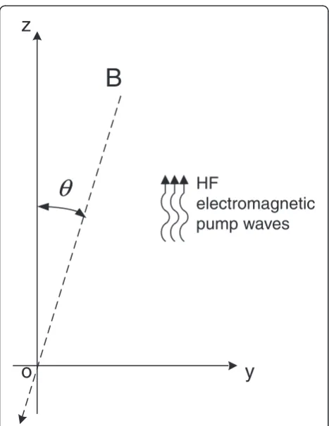
The general equation for wave propagation in an isotropic inhomogeneous plasma medium can be derived from the Maxwell equations, which are expressed in the Cartesian coordinate system in the form (Gurevich, 1978):
Δ→E −∇ ∇ ●→Eþω
tensor andω is the wave angular frequency. When con-sidering a plane electromagnetic wave impinging verti-cally upon the ionosphere, the changes in E→depend on thez-coordinate only. Then, Eq. (1) can be rewritten as:
d2E
This equation is applicable to both of the horizontal E→
components,ExandEy. When the background ionosphere
is considered to be a linear plasma layer without absorp-tion, Eq. (2) becomes:
ε0ðω;zÞ ¼εð Þ ¼z n2
z
ð Þ;σ¼0: ð3Þ
where n2 is the square of the complex refractive index. Ex and Ey are determined from the one-dimensional time-independent wave equation:
In this paper, we are interested in analyzing the
X¼ω2pe=ω2;Y¼ωce=ω;Z¼ν=ω; ð5Þ
whereωpe andωceare the electron plasma (angular) fre-quency and the electron cyclotron frefre-quency, respect-ively. For the specific expressions of these two terms, refer to Rishbeth and Garriott 1969. The electron colli-sion frequency νe=νem+νei, where νem and νei are the collision frequencies of electrons with neutral particles and with ions, respectively. The specific expressions of these collision frequencies are given in detail in Banks and Kocharts1973and Schunk and Walker1980.
The wave equations for the components of E→ can be derived from Maxwell’s equations in the usual, well-known way, as we have discussed above. Assuming a time variation of exp[−iωt], we obtain the following wave equations (Ginzburg, 1970):
d2Ex
dz2 þk 2
Q11ð Þz Exþk2Q12ð Þz Ey¼0; ð6aÞ
d2Ey
dz2 þk 2
Q21ð Þz Exþk2Q22ð Þz Ey ¼0; ð6bÞ
EzþQ31ð Þz ExþQ32ð Þz Ey¼0; ð6cÞ
where the functionsQij(z) are given by
Q11ð Þ ¼z 1−X z
ð Þ½1þiZ½1þiZ−X zð Þ
D zð Þ ;
Q12ð Þ ¼z −Q21ð Þ ¼z −iX z
ð Þ½1þiZ−X zð ÞYcosθ
D zð Þ ;
Q22ð Þ ¼z 1−
X zð Þ½1þiZ½1þiZ−X zð Þ D zð Þ
þX zð ÞY2sin2θ
D zð Þ ;
Q31ð Þ ¼z iX z
ð Þ½1þiZYsinθ
D zð Þ ;
Q32ð Þ ¼z −
X zð ÞY2sinθcosθ
D zð Þ ;
with the common denominator
D zð Þ ¼½1þiZ−X zð Þð1þiZÞ2−Y2−X zð ÞY2sin2θ: ð7Þ
We can easily see that wave Eqs. (6a) and (6b) are coupled and, therefore, it is a formidable task to obtain exact solutions in their current form. However, for a homogeneous medium, the exact solution of (6a) and (6b) can be obtained trivially by solving the eigenvalue problem of the corresponding matrix, which is then constant. This yields the eigenvalues (Lundborg and Thide, 1986):
n2O=X¼1−
X 2D
n
2 1ð þiZÞð1þiZ−XÞ−Y2sin2θ
∓Y4sin4θþ4 1ð þiZ−XÞ2Y2cos2θ
1 2o;
ð8Þ
and the corresponding eigenvectors described by the transverse polarization
ρ¼Ey=Ex;
ρO=X¼
i
2 1ð þiZ−XÞYcosθ n
Y2sin2θ
Y4sin4θþ4 1ð þiZ−XÞ2Y2cos2θ
1 2o:
ð9Þ
The lower subscripts and signs∓(or ±) in Eqs. (8) and (9) correspond to the O and X modes, respectively. From Eq. (9), we easily find that the two polarizations satisfyρOρX= 1. For convenience in what follows, we
pri-marily use the quantity ρX in our equations, as ρO
be-comes very large in the O-mode reflection region.
y
z
B
o
θ
HF
electromagnetic
pump waves
The characteristic waves in the homogeneous medium are thus the well-known O- and X-mode wave with complex wave numbers knO or knX, according to (8),
and with polarizations given by (9). However, it must be remembered that, in an inhomogeneous medium, these waves are no longer exact solutions of the wave equations. Obviously, the pump-wave reflection area in our calculation no longer satisfies this condition. How-ever, if the medium is slowly varying, one might hope that there exist approximate solutions under certain conditions corresponding to the characteristic modes that are at least less strongly coupled to each other than the Cartesian field components. It might therefore be a good idea to transform the dependent variablesEx
andEyin (6a) and (6b) to new variables corresponding
to the characteristic wave modes for a homogeneous plasma. The specific conversion procedure is described in both Lundborg and Thide 1986 and Budden 1966. Hence, we express the transverse field in terms of the two Forsterling functionsFOandFX, where:
Ex¼ρXEy;OþEx;X;Ey¼Ey;OþρXEx;X;
The new variablesFOandFXin Eq. (10) must satisfy
F00Oþ k2n2Oþq2
where the coupling functionqis defined as
q¼ i iZ
Equations (11a) and (11b) are the Forsterling equa-tions, which contain no approximations and, hence, are equivalent to the original equations, (6a) and (6b). Assuming the solutions of Eqs. (11a) and (11b) are known, we obtain Ex and Ey from Eq. (10) and,
finally, Ez from Eq. (6c). We can then achieve a
for-mal simplification of these results by introducing the longitudinal polarization
ρL¼Ez=Ex: ð13Þ
Substituting (13) into Eqs. (6c) and (10) yields
ρL;O=X¼
We may now write the exact total field in the form
E¼EOþEX;
The new approach presented here describes the E→ com-ponents of the characteristic waves by utilizing the For-sterling functions discussed above. For our purposes, the wave Eqs. (11a) and (11b) are in a more suitable form than Eqs. (6a) and (6b), since the coupling, which is expressed in terms ofq, is sufficiently small in our appli-cations to be neglected. Indeed, according to Eq. (12),q
is proportional to iZ'−X', which is very small in the slowly varying medium we have chosen. Hence, in such a medium, Eqs. (11a) and (11b) can in good approxima-tion be treated as two uncoupled equaapproxima-tions, where
FO00þk2nO2FO¼0; ð16aÞ
FX00þk2nX2FX ¼0: ð16bÞ
These are the wave equations for the well-known characteristic modes, i.e., the O and X modes, respect-ively. It can be seen that the forms of these wave equa-tions are almost exactly identical to that of Eq. (4). In the present paper, these equations are treated using a more comprehensive and versatile uniform approxima-tion method, which can provide accurate soluapproxima-tions that are valid throughout entire reflection regions.
In order to apply this method, we consider a differential equation in the following form (Berry and Mount, 1972):
d2ψ dϕ2þk
2
P2ð Þϕ ψ¼0; ð17Þ
whereϕ(z) is the mapping function,Pis the phase value of theϕ(z) andψ is the potential value, the solutions of ψ has known and Eq. (17) is our so-called “comparison equation”. Next, we express the solutions of wave Eq. (16a) in terms of the knownψin the form:
n2ð Þ ¼z dϕ
exactly. Thus, Eq. (18) gives the exact solution ofFO(z). IfP2(ϕ) is appropriately chosen,ϕ(z) will be slowly vary-ing and the second term on the right-hand side of n2(z) may be neglected on account of the first. Hence, we ob-tain the first approximation
dϕ
dz ¼
n zð Þ
Pð Þϕ : ð20Þ
As this method functions only if the transition points of the two wave equations correspond to each other, we may defineϕ(z) implicitly, using Eq. (17), from
ζ¼k
Here, we introduce the intermediary variableζ=ζ(ϕ) =ζ(ϕ(z)). Hence, ϕ1 is obviously the zero (transition
point) ofP2(ϕ) that corresponds to the zerot1ofn2(z). In the case of only a single complex reflection point, we can choose the Airy equation as our comparison equation, where:
d2ψ
dϕ2−ϕψ¼0; ð22Þ
Here, we have k2P2(ϕ) =−ϕ, with the zero ϕ1= 0
cor-responding to the zerot1ofn2(z) in Eq. (4). By means of Eqs. (17) and (21), we then obtain
ϕð Þ ¼z −3i 2ζ
2
3
: ð23Þ
The general solution of Eq. (17) can be expressed in terms of the Airy functions (Abramowitz and Stegun, 1972), such that:
ψ ϕð Þ ¼αAið−Reϕð Þz Þ þβBið−Reϕð Þz Þs ð24Þ
whereαand βare the normalizing factor and the Stokes coefficient respectively, and the factor α is defined as (Hinkel et al.1992):
Here, zn is the base point of the ionosphere and the
value of En is the field intensity at zn, which is
deter-mined by the effective radiated power (ERP) value and the non-deviation absorption of the HF pump waves. The physical conditions require the solutionFO(z) of Eq.
(18) to decay asz→∞and, hence, we must choose a ψ solution that decays in the jargϕj<π3 region, i.e., we
requireβ= 0. From Eqs. (18), (19), and (24), we thus ob-tain the first-order uniform solution ofFO(z), such that:
FOð Þ ¼z α −ϕð Þz
k2n2 Oð Þz
" #
Aið−Reϕð Þz Þ: ð26Þ
As we have already mentioned, the solution technique utilizing a uniform approximation of the wave equation, what we discussed above can also be used to treat the X mode.
Results and discussion
The approximation method discussed above can only be employed to derive the solutions for the particular case having one complex zero of n2(z). This is because the applicability of the uniform approximation method is in-herently connected to the behaviors of functions (19) and (21). The O-mode refractive index has a zero when
X¼1þiZ; ð27aÞ
i.e., at the same points as for a corresponding nonmag-netic medium. The X-mode refractive index is zero when
X¼1þiZ−Y: ð27bÞ
In this paper, we only analyze the variation of the field intensities of the HF pump-wave standing wave patterns for over-dense heating mode. In this case, the emission frequencies of powerful pump waves from the transmitter are less than the critical frequency value of the ionospheric F2 layer f0F2, and the pump-wave re-flection heights are lower than the density peak of the F2 layer hmF2. As the pump-wave reflection heights in
our calculation lie in the F layer of the ionosphere, where the electron density monotonically increases with height, we assume that the electron density profile is a linear monotonic case, such that:
X¼1þz−z0
h ; ð28Þ
wherez0is the reflection point (the real part of the
com-plex transition point) of O-mode waves and h is the scale length of the profile.
From the Eyand Ezcomponents of E
→
in Eq. (15), we obtain its components perpendicular and parallel to the geomagnetic field as
E⊥¼ cosθEyþ sinθEz; ð29Þ
E∥¼−sinθEyþ cosθEz; ð30Þ
parameters chosen for our simulation are listed in detail for three locations in Table1.
As shown above, not only the parameters of the F region at Alaska, Wuhan, and Haikou (three daytime (LT = 1400) locations corresponding to different latitude areas) were chosen for our calculation but also the pa-rameters of the Wuhan area at night (LT = 0200). The latter were selected in order to study the impact of the day–night differences in the ionospheric background pa-rameters on the distribution of the HF pump waves. Here, the emission frequency of the pump wave was chosen to be 0.9 times the localf0F2, and the ERP of the pump waves was set to 10 MW. Note that the upper-hybrid resonance altitude listed in the last line of Table 1 was included in the calculation interval for the O-mode waves, as many nonlinear phenomena, such as field-aligned irregularities, optical emissions, and stimulated electromagnetic emissions, are influenced by the upper-hybrid resonance. This resonance occurs at the altitude where the upper-hybrid resonance frequencyωUHequals
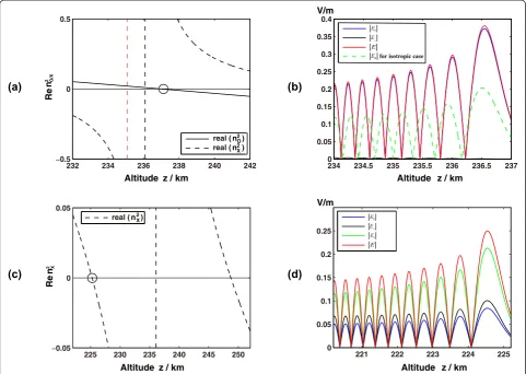
ω, and ω2UH ¼ω2peþω2ce. The simulation results for the three locations in daytime are shown in Figs. 2, 3, and 4, while the real parts of the refractive index function for the O and X modes n2
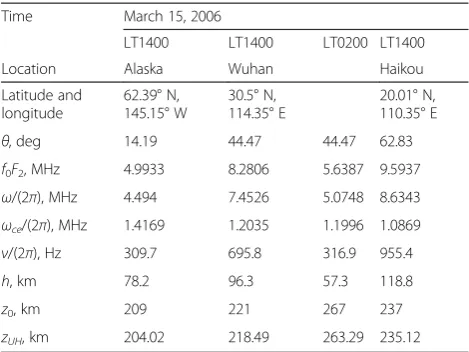
O=Xð Þz are also presented in the Figs. 2a, c, 3a, c, and 4a, c.
The red dashed vertical line in Fig. 2a represents the location of the upper-hybrid resonance altitude.
In Fig. 2a, the real part of n2
O is far from linear. The function is rather smooth, whereas its derivative under-goes a rapid change in the region around z0, where the
value of n2O has a zero (z=z0= 209 km; the black circle shown in the figure). However, the derivative remains monotonic. Furthermore, we find that the refractive index of the X-mode wavesn2
X goes to infinity before the O-mode wave reflection point (z= 208.4 km; the black dashed vertical line in Fig. 2a); this is referred to as the
plasma resonance region. It can be seen that theE→ com-ponents of the O-mode waves vary rapidly in the region
beforez0. The E→component parallel to the geomagnetic field E∥ plays a dominant role in all components and
undergoes obvious growth (the blue solid curve in
Fig. 2b), which leads to a rapid increase in the totalE→ in-tensity; this is usually referred to as swelling. At the same time, the component perpendicular to the geomag-netic fieldE⊥decreases rapidly in the region nearz0(the
black solid curve in Fig. 2b), and almost vanishes at z0
itself. It is also found that the total electric field |E| (the red solid curve in Fig. 2b) varies more rapidly and has a larger amplitude than the electric field for the isotropic case |E0| (the green dashed curve in Fig. 2b), when the geomagnetic field is neglected. Here, we define the pump-wave swelling factor, which is the ratio of the
maximum E→ amplitudes before the reflection height to the empirical value. The latter is normally calculated using the empirical model, as a function of altitude from the pump-wave ERP, i.e.,E≈0:25pffiffiffiffiffiffiffiffiffiERP=z(Gurevich, 1978; Robinson, 1989). The swelling factor of the O-mode waves for the Alaska case is approximately 10.97.
In Fig. 2c, the value ofn2
X has a zero before the reflec-tion point of the O-mode waves (z= 184.3 km, the black circle shown in the figure), indicating that the X-mode waves do not usually reach the reflection level of the
O-mode waves. The E→ components of the X-mode waves exhibit significantly different behavior, in that E∥ (the
blue solid curve in Fig. 2d) is significantly smaller than the other two components, E⊥ and Ex (indicated by the
black and green solid curves in Fig. 2d, respectively),
which are perpendicular to the geomagnetic field. All E→
components of the X-mode waves are not enhanced significantly in the vicinity of its reflection point, which results in a reduced field swelling effect. The swelling factor for the X-mode waves in Alaska is approximately 4.05.
From Eq. (9), we can see that the value of ρO is
ap-proximately equal to i for variable z is not too close to the z0 and Y≪1. Hence, the transverse part of the
upgoing O-mode waves is, to a good approximation, cir-cularly polarized in the right-hand sense. On the other hand, forzvalue that is very close to thez0,X≈1,n2
O≈0, and Z≪Y, and we can obtain the following approxima-tion from Eqs. (9) and (14)
Table 1Selected parameters for linear profile model of F region at Alaska, Wuhan, and Haikou
Time March 15, 2006
f0F2, MHz 4.9933 8.2806 5.6387 9.5937
ω/(2π), MHz 4.494 7.4526 5.0748 8.6343
ωce/(2π), MHz 1.4169 1.2035 1.1996 1.0869
ν/(2π), Hz 309.7 695.8 316.9 955.4
h, km 78.2 96.3 57.3 118.8
z0, km 209 221 267 237
zUH, km 204.02 218.49 263.29 235.12
ρX≈Zcosθ
Ysin2θ;ρL;O≈−
Ysinθ
Z : ð31Þ
According to Eqs. (15), (29), and (30), this means that at exactlyz0and in its immediate vicinity
E∥¼−sinθEyþ cosθEz
¼−sinθEyþ cosθ•ρXρLOEy
≈ −sinθ−cos
2θ
sinθ
Ey ¼−
1 sinθEy;
ð32Þ
Analogously,
E⊥¼ cosθEyþ sinθEz
¼cosθþ sinθ•ρXρLOEy
≈cosθ−sinθcosθ sinθ
Ey¼0:
ð33Þ
The above discussion gives a distinct explanation of why the E⊥ component goes to zero at z0, and shows
that →E becomes almost aligned with the geomagnetic field very near z0. In addition, its propagation vector
becomes perpendicular to the geomagnetic field B0, also because of this field orientation near z0. Thus, the electromagnetic wave can easily couple to electro-static mode waves such as Langmuir or ion-acoustic waves, resulting in various instabilities (Ginzburg, 1970; Rietveld et al. 1993).
For X-mode waves, also from Eq. (28), we can see that for z values very close to the X-mode wave reflection pointz0−hY, thenX→1−Y, and |1−X|≃Y. Therefore, we can obtain the approximation from Eqs. (9) and (14), such that:
ρX≈−icosθ;ρL;X≈−
iYsinθ
YþiZ: ð34Þ
The equations above clearly indicate that |ρX| < 1 and
|ρL,X| < 1. Therefore, combining these expressions with
Eq. (15) may give a distinct explanation of why the E→
component perpendicular to the magnetic meridian (a)
(c)
(b)
(d)
plane Ex (the green solid curve in Fig. 2d) is greater
than the other two field components in the magnetic meridian plane (the black and blue solid curves in Fig. 2d). In addition, the coefficients obtained in Eq. (34) can be compared to the corresponding coeffi-cients of the O-mode waves in Eq. (31); this may ex-plain why only a reduced field swelling effect is observed for the X-mode waves. As the value of θ in-creases as theYcomponent decreases with decreasing
latitude, the swelling effect of the E→ components of the X-mode waves decreases with decreasing latitude.
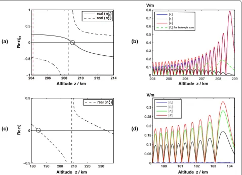
The red dashed vertical line in Fig. 3a represents the location of the upper-hybrid resonance altitude.
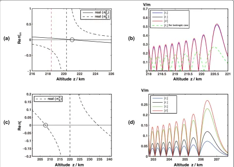
The red dashed vertical line in Fig. 4a represents the location of the upper-hybrid resonance altitude.
The standing wave patterns of the characteristic waves formed near their reflection points in the Wuhan and Haikou areas in daytime (LT = 1400) are illustrated in Figs. 3 and 4, for the parameters given in columns 2 and 4 of Table 1, respectively. Comprehensive analysis
considering Figs. 2, 3, and 4 shows that the reflection heights of both characteristic waves increase and the distance between them decreases with decreasing lati-tude (the black circles in Figs. 3a, c and 4a, c above). In addition, the values of the real parts of n2O and n2X continue to monotonically decrease with height before each reflection point. Furthermore, the distance between the O-mode reflection point z0 and the upper-hybrid resonance altitude also decreases with decreasing lati-tude, as can be concluded from the parameters listed in the last line of Table 1. The parallel component E∥ of
the O-mode waves continues to play a dominant role in each of the field components and the swelling effect of
E →
decreases with decreasing latitude. The amplitude of theE∥ component in Fig. 4a for the Haikou area is
sig-nificantly less than that for Alaska, which is shown in Fig. 2a. The swelling factor of the O-mode waves also decreases with decreasing latitude, and the O-mode wave swelling factor in Haikou is only 4.5. Because of the close distance between the upper-hybrid resonance (a)
(c)
(b)
(d)
altitude andz0in the lower latitude area, the amplitude of |E| at the upper-hybrid resonance altitude is even
higher than its value atz0. This is because E→ begins to decay before the reflection point is reached.
The electron density and temperature in the back-ground ionosphere, along with the electron collision fre-quency, may increase with decreasing latitude; this implies that the HF pump-wave emission frequency ex-hibits a relative growth, while the value of the geomag-netic field may decrease with decreasing latitude. This causes the value of the Ycomponent and the distance between the X- and O-mode reflection points to grad-ually decrease with decreasing latitude. The value of θ may also increase with decreasing latitude. All of the reasons given above may explain why the amplitude of the E∥ component of the O-mode waves and the swell-ing effect of |E| gradually decrease with decreasing lati-tude. Further, the above discussion may also explain why the distance betweenz0and the upper-hybrid resonance
altitude also decreases with decreasing latitude.
For X-mode waves, the amplitude ofExis greater than
the other two components in the magnetic meridian plane. In addition, the swelling effect of all components is significantly weaker than in the O-mode wave case. Thus, only a reduced field swelling effect is formed in the vicinity of its reflection point, and the swelling factor for the X-mode waves is less than half that of the O-mode waves.
We have shown the standing wave pattern results for a partially or totally reflected HF wave impinging verti-cally upon the ionosphere, which were calculated using the “uniform approximation” method within the linear electron density profile at different latitude areas in daytime. However, in addition to the impact of the lati-tude, the effect of the day–night differences on the ionospheric background parameters is also very obvi-ous. In order to study the impact of these differences on the distribution of the HF pump waves, we present the simulation result for the Wuhan area at night in Fig. 5. The parameters used here are given in column 3 (a)
(c)
(b)
(d)
of Table 1. The emission frequency of the pump wave was again set to 0.9 times the localf0F2, and the ERP of the pump waves was 10 MW.
The red dashed vertical line in Fig. 5a represents the location of the upper-hybrid resonance altitude.
An analysis comparing the results shown in Figs. 3 and 5 shows that the characteristic-wave reflection height at night is significantly greater than the daytime value. In addition, more intensive variations occur in the real part values ofn2
O andn2X at night. The swelling of the E→ components for the O- and X-mode waves in the vicinity of each reflection points are significantly
larger than those during the daytime, and the total E→
intensity can reach significantly higher values at night. As regards the background electron density and elec-tron temperature of the ionosphere, the elecelec-tron colli-sion frequencies at nighttime are significantly lower than those in daytime; this implies that the HR pump-wave emission frequency has a relatively lower value.
Although the circadian variations of B0 are not obvi-ous, the above behaviors cause a sharp increase in the value of theYcomponent, the distance between the O-and X-mode reflection points, O-and in the upper-hybrid resonance altitude. In addition, the decrease in the value of the background electron density and the elec-tron temperature of the ionosphere cause a reduction in the background absorption and the energy loss of the HF pump waves. That is, the energy in the vicinity of the reflection points and the field intensity of the standing wave pattern of the characteristic waves are much larger.
Conclusions
In this paper, we have demonstrated the application of the“uniform approximation”method and the Forsterling equation for investigation of the standing wave pattern of a partially or totally reflected HF wave impinging ver-tically upon the ionosphere, at different latitudes and also at different local times in a single location. The (a)
(c)
(b)
(d)
numerical results show that the value of the real part of
n2O monotonically decreases with height, while the value of the real part of n2
X also monotonically decreases be-fore its reflection point. Further, the distance between the X- and O-mode wave reflection points decreases with decreasing latitude. It is also found that the
swell-ing of the E→ components of the characteristic waves is much larger and the distance between these maxima is much shorter than in the isotropic case, where the geo-magnetic field is neglected. The swelling factors of the pump waves are larger at higher latitudes than at lower ones. Our results suggest that the ionospheric back-ground parameters and the inclination and intensity of the geomagnetic field may have an important effect on
the amplitude and spatial distributions of the E→ of HF pump waves.
The ERP value of the HF pump waves is set to
10 MW in our calculation. The E→ at the standing wave maxima nearz0reaches a magnitude of hundreds of mV per meter, exceeding by far the threshold values for cer-tain instabilities (e.g., thermal self-focusing, resonant, and parametric instability) (Kuo, 2015). The intense wave field modifies the plasma density at these maxima. The approximation calculation results in this paper can be used to derive the precise ERP values of HF pump waves used to excite all kinds of instabilities, and also function as a theoretical reference for ionospheric modulation experiments in future.
Competing interests
The authors declare that they have no competing interests.
Authors’contributions
CW performed the derivation of the theoretical equations, wrote the computational program, and drafted the manuscript. CZ conceived the study and proofread the manuscript. ZYZ corrected the errors in the original equations and discussed the results with the authors. XBY helped to solve problems and bugs in the computational program. All authors have read and approved the final manuscript.
Received: 21 May 2015 Accepted: 29 June 2015
References
Abramowitz M, Stegun IA (1972) Handbook of mathematical functions. Dover Press, New York
Banks PM, Kocharts G (1973) Aeronomy, Parts A and B. Academic Press, New York Berry MV, Mount KE (1972) Semiclassical approximations in the wave mechanics.
Rep Prog Phys 35:315–397
Budden KG (1966) Radio waves in the ionosphere. Cambridge University Press, New York
Fejer JA (1979) Ionospheric modification and parametric instabilities. Rev Geophys 17:135–153
Fejer JA (1981) Correction to“Ionospheric modification and parametric instabilities”. Rev Geophys 19:344–359
Fejer JA, Ierkic HM, Woodman RF, Rottger J, Sulzer M, Behnke RA, Veldhuis A (1983) Observations of the HF-enhanced plasma line with a 46.8 MHz radar and reinterpretation of previous observations with the 430 MHz radar. J Geophys Res 88:2083–2092
Field EC, Bloom RM, Kossey PA (1990) Ionospheric heating with oblique high-frequency waves. J Geophys Res 95(A12):21179–21186
Ginzburg VL (1970) The propagation of electromagnetic waves in plasmas, 2nd edn. Pregamon, New York
Gondarenko NA, Guzdar PN, Ossakow SL, Brenhardt PA (2003) Linear mode conversion in inhomogeneous magnetized plasmas during ionospheric modification by HF radio waves. J Geophys Res 108(A12):1470–1485. doi:10.1029/2003JA009985
Gondarenko NA, Guzdar PN, Ossakow SL, Brenhardt PA (2004) Perfectly matched layers for radio wave propagation in inhomogeneous magnetized plasmas. J Comput Phys 194:481–504
Gurevich AV (1978) Nonlinear phenomena in the ionosphere. Spring-Verlag, Berlin Hao SJ, Li QL, Yang JT, Wu ZS (2013) Theory and numerical modeling of
under-dense heating with powerful X-mode pump waves. Chinese J Geophys 56(8):2503–2510
Hinkel DE, Shoucri MM, Smith TM, Wagner TM (1992) Modeling of HF propagation and heating in the ionosphere. Rome Laboratory of US Air Force, New York
Hinkel DE, Shoucri MM, Smith TM, Wagner TM, Hansen JD, Morales GJ (1993) Modeling of high-frequency oblique propagation and heating in the ionosphere. Radio Sci 28(5):819–837
Huang WG, Gu SF (2003) The heating of upper ionosphere by powerful high-frequency radio waves. Chin J Space Sci 23(5):343–351
Kuo SP (2015) Ionospheric modifications in high frequency heating experiments. Phys Plasma 22:012901. doi:10.1063/1.4905519, 2015
Langer RE (1937) On the connection formulas and solutions of the wave equation. Phys Rev 51:669–676
Lundborg B, Thide B (1985) Standing wave pattern of HF radio waves in the ionospheric reflection region 1. General Formulas Radio Sci 20(4):947–958 Lundborg B, Thide B (1986) Standing wave pattern of HF radio waves in the
ionospheric reflection region 2. Applications Radio Sci 21(3):486–500 Miller SC, Good RH (1953) A WKB-type approximation to the Schrodinger equation.
Phys Rev 91:174–179
Rietveld MT, Kohl H, Kopka H et al (1993) Introduction to ionospheric heating at Tromsφ–I. Experimental overview. J Atmos Sol-Terr Phy 55:577–599 Rishbeth H, Garriott OK (1969) Introduction to ionospheric physics. Academic
Press, Waltham
Robinson TR (1989) The heating of the high latitude ionosphere by high power radio waves. Elsevier Science Publishers, Amsterdam
Schunk RW, Walker JC (1980) Theoretical ion densities in the lower ionosphere. Space Phys 18:813–820
Stubbe P, Kopka H, Thide B, Derblom H (1984) Stimulated electromagnetic emission: a new technique to study the parametric decay instability in the ionosphere. J Geophys Res 89:7523–7536
Utlaut WF (1970) An ionospheric modification experiments at Tromsφ. J Geophys Res 75(31):6402–6405
Utlaut WF, Cohen R (1971) Modifying the ionosphere with intense radio waves. Science 174:245–254
Utlaut WF, Violette EJ (1972) Further observations of ionospheric modification by a high powered HF transmitter. J Geophys Res 77:6804–6818
Submit your manuscript to a
journal and benefi t from:
7 Convenient online submission
7 Rigorous peer review
7 Immediate publication on acceptance
7 Open access: articles freely available online
7 High visibility within the fi eld
7 Retaining the copyright to your article