High-Level Synthesis of DSP Applications
Using Adaptive Negative Cycle Detection
Nitin Chandrachoodan
Department of Electrical and Computer Engineering, University of Maryland, College Park, MD 20742, USA Email: [email protected]
Shuvra S. Bhattacharyya
Department of Electrical and Computer Engineering, University of Maryland, College Park, MD 20742, USA Email: [email protected]
K. J. Ray Liu
Department of Electrical and Computer Engineering, University of Maryland, College Park, MD 20742, USA Email: [email protected]
Received 31 August 2001 and in revised form 15 May 2002
The problem of detecting negative weight cycles in a graph is examined in the context of thedynamic graphstructures that arise in the process of high level synthesis (HLS). The concept ofadaptivenegative cycle detection is introduced, in which a graph changes over time and negative cycle detection needs to be done periodically, but not necessarily after every individual change. We present an algorithm for this problem, based on a novel extension of the well-known Bellman-Ford algorithm that allows us to adapt existing cycle information to the modified graph, and show by experiments that our algorithm significantly outperforms previous incremental approaches for dynamic graphs. In terms of applications, the adaptive technique leads to a very fast imple-mentation of Lawlers algorithm for the computation of the maximum cycle mean (MCM) of a graph, especially for a certain form of sparse graph. Such sparseness often occurs in practical circuits and systems, as demonstrated, for example, by the ISCAS 89/93 benchmarks. The application of the adaptive technique to design-space exploration (synthesis) is also demonstrated by developing automated search techniques for scheduling iterative data-flow graphs.
Keywords and phrases:negative cycle detection, dynamic graphs, maximum cycle mean, adaptive performance estimation.
1. INTRODUCTION
High-level synthesis of circuits for digital signal processing (DSP) applications is an area of considerable interest due to the rapid increase in the number of devices requiring multi-media and DSP algorithms. High-level synthesis (HLS) plays an important role in the overall system synthesis process be-cause it speeds up the process of converting an algorithm into an implementation in hardware, software, or a mixture of both. In HLS, the algorithm is represented in an abstract form (usually a dataflow graph), and this representation is transformed and mapped onto architectural elements from a library of resources. These resources could be pure hardware elements like adders or logic gates, or they could be general purpose processors with the appropriate software to execute the required operations. The architecture could also involve a combination of both the above, in which case the problem becomes one of hardware-software cosynthesis.
HLS involves several stages and requires computation of
several parameters. In particular, performance estimation is one very important part of the HLS process, and the actual design space exploration (synthesis of architecture) is an-other. Performance estimation involves using timing infor-mation about the library elements to obtain an estimate of the throughput that can be obtained from the synthesized implementation. A particularly important estimate for iter-ative dataflow graphs is known as the maximum cycle mean (MCM) [1, 2]. This quantity provides a bound on the max-imum throughput attainable by the system. A fast method for computing the MCM would therefore enable this metric to be computed for a large number of system configurations easily.
-ciently good solutions. An important feature of HLS of DSP applications is that the mapping to hardware needs to be done only once for a given design, which is then produced in large quantities for a consumer market. As a result, for these applications (such as modems, wireless phones, multimedia terminals, etc.), it makes sense to consider the possibility of investing large amounts of computational power at compile time, so that a more optimal result can be used at run time.
The problems in HLS described above both have the common feature of requiring a fast solution to the problem of detecting negative cycles in a graph. This is because the execution times of the various resources combine with the graph structure to impose a set of constraints on the system, and checking the feasibility of this set of constraints is equiv-alent to checking for the presence of negative cycles in the corresponding constraint graph.
DSP applications, more than other embedded applica-tions considered in HLS, have the property that they are
cyclic in nature. As explained in Section 2, this means that the problem of negative cycle detection in constraint analy-sis is more relevant to such systems. In order to make use of the increased computational power that is available, one pos-sibility is to conduct more extensive searches of the design space than is performed by a single heuristic. One possible approach to this problem involves an iterative improvement system based on generating modified versions of an existing implementation and verifying their correctness. The incre-mental improvements can then be used to guide a search of the design space that can be tailored to fit in the maximum time allotted to the exploration problem. In this process, the most computationally intensive part is the process of verify-ing correctness of the modified systems, and therefore speed-ing up this process would have a direct impact on the size of the explored region of the design space.
In addition to these problems from HLS, several other problems in circuits and systems theory require the solv-ing of constraint equations [2, 3, 4, 5, 6]. Examples include very large scale integrated circuit (VLSI) layout compaction, interactive (reactive) systems, graphic layout heuristics, and timing analysis and retiming of circuits for performance or area considerations. Though a general system of constraints would require a linear programming (LP) approach to solve it, several problems of interest actually consist of the special case of difference constraints (each constraint expresses the minimum or maximum value that the difference of two vari-ables in the system can take). These problems can be attacked by faster techniques than the general LP, mostly involving the solution of a shortest path problem on a weighted directed graph. Detection of negative cycles in the graph is therefore a closely related problem, as it would indicate the infeasibility of the constraint system.
Because of the above reasons, detecting the presence of negative cycles in a weighted directed graph is a very im-portant problem in systems theory. This problem is also important in the computation of network flows. Consider-able effort has been spent on finding efficient algorithms for this purpose. Cherkassky and Goldberg [3] have performed a comprehensive survey of existing techniques. Their study
shows some interesting features of the available algorithms, such as the fact that for a large class of random graphs, the worst case performance bound is far more pessimistic than the observed performance.
There are also situations in which it is useful or neces-sary to maintain a feasible solution to a set of difference con-straints as a system evolves. Typical examples of this would be real-time or interactive systems, where constraints are added or removed one (or several) at a time, and after each such modification it is required to determine whether the result-ing system has a feasible solution and if so, to find it. In these situations, it is often more efficient to adapt existing infor-mation to aid the solution of the constraint system. In the example from HLS that was mentioned previously, it is pos-sible to cast the problem of design space exploration in a way that benefits from this approach.
Several researchers [5, 7, 8] have worked on the area of
incremental computation. They have presented analyses of al-gorithms for the shortest path problem and negative cycle detection indynamicgraphs. Most of the approaches try to apply the modifications of Dijkstra’s algorithm to the prob-lem. The obvious reason for this is that this is the fastest known algorithm for the problem when only positive weights are allowed on edges. However, the use of Dijkstra’s algo-rithm as the basis for incremental computation requires the changes to be handled one at a time. While this may often be efficient enough, there are many cases where the ability to handle multiple changes simultaneously would be more advantageous. For example, it is possible that in a sequence of changes, one reverses the effect of another: in this case, a normal incremental approach would perform the same com-putation twice, while a delayed adaptive comcom-putation would not waste any effort.
In this paper, we present an approach that generalizes the adaptive approach beyond single increments: we address multiple changes to the graph simultaneously. Our approach can be applied to cases where it is possible to collect several changes to the graph structure before updating the solution to the constraint set. As mentioned previously, this can re-sult in increased efficiency in several important problems. We present simulation results comparing our method against the single-increment algorithm proposed in [4]. For larger num-bers of changes, our algorithm performs considerably better than this incremental algorithm.
To illustrate the advantages of our adaptive approach, we present two applications from the area of HLS, requiring the solution of difference constraint problems, which therefore benefit from the application of our technique. For the prob-lem of performance estimation, we show how the new tech-nique can be used to derive a fast implementation of Lawler’s algorithm [9] for the problem of computing the MCM of a weighted directed graph. We present experimental results comparing this against Howard’s algorithm [2, 10], which appears to be the fastest algorithm available in practice. We find that for graph sizes and node-degrees similar to those of real circuits, our algorithm often outperforms even Howard’s algorithm.
search technique for finding schedules for iterative dataflow graphs that uses the adaptive negative cycle detection al-gorithm as a subroutine. We illustrate the use of this local search technique by applying it to the problem of resource-constrained scheduling for minimum power in the presence of functional units that can operate at multiple voltages. The method we develop is quite general and can therefore easily be extended to the case of optimization where we are inter-ested in optimizing other criteria rather than the power con-sumption.
This paper is organized as follows. Section 2 surveys previous work on shortest path algorithms and incremen-tal algorithms. In Section 3, we describe the adaptive algo-rithm that works on multiple changes to a graph efficiently. Section 4 compares our algorithm against the existing ap-proach, as well as against another possible candidate for adaptive operation. Section 5 then gives details of the appli-cations mentioned above, and presents some experimental results. Finally, we present our conclusions and examine ar-eas that would be suitable for further investigation.
A preliminary version of the results presented in this pa-per were published in [11].
2. BACKGROUND AND PROBLEM FORMULATION Cherkassky and Goldberg [3] have conducted an extensive survey of algorithms for detecting negative cycles in graphs. They have also performed a similar study on the problem of shortest path computations. They present several prob-lem families that can be used to test the effectiveness of a cycle-detection algorithm. One surprising fact is that the best known theoretical bound (O(|V||E|), where|V|is the number of vertices and |E| is the number of edges in the graph) for solving the shortest path problem (with arbitrary weights) is also the best known time bound for the negative cycle problem. But examining the experimental results from their work reveals the interesting fact that in almost all of the studied samples, the performance is considerably less costly than would be suggested by the product|V| × |E|. It appears that the worst case is rarely encountered in random exam-ples, and an average case analysis of the algorithms might be more useful.
Recently, there has been increased interest in the sub-ject ofdynamicorincrementalalgorithms for solving prob-lems [5, 7, 8]. This uses the fact that in several probprob-lems where a graph algorithm such as shortest paths or transi-tive closure needs to be solved, it is often the case that we need to repeatedly solve the problem on variants of the origi-nal graph. The algorithms therefore store information about the problem that was obtained during a previous iteration and use this as an efficient starting point for the new prob-lem instance corresponding to the slightly altered graph. The concept ofbounded incremental computationintroduced in [7] provides a framework within which the improvement af-forded by this approach can be quantified and analyzed.
In this paper, the problem we are most interested in is that of maintaining a solution to a set of difference con-straints. This is equivalent to maintaining a shortest path
tree in a dynamic graph [4]. Frigioni et al. [5] present an al-gorithm for maintaining shortest paths in arbitrary graphs that performs better than starting from scratch, while Rama-lingam and Reps [12] present a generalization of the short-est path problem, and show how it can be used to handle the case where there are few negative weight edges. In both of these cases, they have considered one change at a time (not multiple changes), and the emphasis has been on the theoretical time bound, rather than experimental analysis. In [13], the authors present an experimental study, but only for the case of positive weight edges, which restricts the study to computation of shortest paths and does not consider nega-tive weight cycles.
The most significant work along the lines we propose is described in [4]. In this, the authors use the observation that in order to detect negative cycles, it is notnecessaryto main-tain a tree of the shortest paths to each vertex. They suggest an improved algorithm based on Dijkstra’s algorithm, which is able to recompute a feasible solution (or detect a negative cycle) in timeO(E+VlogV), or in terms ofoutput complexity
(defined and motivated in [4])O(∆+|∆|log|∆|), where |∆| is the number of variables whose values are changed and∆is the number of constraints involving the variables whose values have changed.
The above problem can be generalized to allow multiple changes to the graph between calls to the negative cycle de-tection algorithm. In this case, the above algorithms would require the changes to be handled one at a time, and therefore would take time proportional to the total number of changes. On the other hand, it would be preferable if we could obtain a solution whose complexity depends on the number of up-datesrequested, rather than the total number of changes ap-plied to the graph. Multiple changes between updates to the negative cycle computation arise naturally in many interac-tive environments (e.g., if we prefer to accumulate changes between refreshes of the state, using the idea of lazy evalua-tion) or in design space-exploration, as can be seen, for ex-ample, in Section 5.2. By accumulating changes and process-ing them in large batches, we remove a large overhead from the computation, which may result in considerably faster al-gorithms.
Note that the work in [4] also considers the addition/ deletion of constraints only one at a time. It needs to be emphasized that this limitation is basic to the design of the algorithm: Dijkstra’s algorithm can be applied only when the changes are considered one at a time. This is accept-able in many contexts since Dijkstra’s algorithm is the fastest algorithm for the case where edge weights are positive. If we try using another shortest paths algorithm we would incur a performance penalty. However, as we show, this loss in per-formance in the case of unit changes may be offset by im-proved performance when we consider multiple changes.
problem of analyzing the sensitivity of the algorithm [14]. The sensitivity analysis tries to study the performance of an algorithm when its inputs are slightly perturbed. Note that there do not appear to be any average case sensitivity anal-yses of the Bellman-Ford algorithm, and the approach pre-sented in [14] has a quadratic running time in the size of the graph. This analysis is performed for a general graph without regard to any special properties it may have. But as explained in Section 5.1.1, graphs corresponding to circuits and systems in HLS for DSP are typically very sparse—most benchmark graphs tend to have a ratio of about 2 edges per vertex, and the number of delay elements is also small rel-ative to the total number of vertices. Our experiments have shown that in these cases, the adaptive approach is able to do much better than a quadratic approach. We also pro-vide application examples to show other potential uses of the approach.
In the following sections, we show that our approach performs almost as well as the approach in [4] (experimen-tally) for changes made one at a time, and significantly out-performs their approach under the general case of multi-ple changes (this is true even for relatively small batches of changes, as will be seen from the results). Also, when the number of changes between updates is very large, our algo-rithm reduces to the normal Bellman-Ford algoalgo-rithm (start-ing from scratch), so we do not lose in performance. This is important since when a large number of changes are made, the problem can be viewed as one of solving the shortest-path problem for a new graph instance, and we should not perform worse than the standard available technique for that. Our interest in adaptive negative cycle detection stems primarily from its application in the problems of HLS that we outlined in the introduction. To demonstrate its useful-ness in these areas, we have used this technique to obtain improved implementations of the performance estimation problem (computation of the MCM) and to implement an it-erative improvement technique for design space exploration. Dasdan et al. [2] present an extensive study of existing al-gorithms for computing the MCM. They conclude that the most efficient algorithm in practice is Howard’s algorithm [10]. We show that the well-known Lawler’s algorithm [9], when implemented using an efficient negative cycle detec-tion technique and with the added benefit of our adaptive negative cycle detection approach, actually outperforms this algorithm for several test cases, including several of the IS-CAS benchmarks, which represent reasonable sized circuits.
As mentioned previously, the relevance of negative cycle detection to design space exploration is because of the cyclic nature of the graphs for DSP applications. That is, there is of-ten a dependence between the computation in one iteration and the values computed in previous iterations. Such graphs are referred to as iterative dataflow graphs[15]. Traditional scheduling techniques tend to consider only the latency of the system, converting it to an acyclic graph if necessary. This can result in loss of the ability to exploit inter-iteration par-allelism effectively. Methods such asoptimum unfolding[16] andrange-chart guided scheduling[15] are techniques that try to avoid this loss in potential parallelism by working directly
on the cyclic graph. However, they suffer from some disad-vantages of their own. Optimum unfolding can potentially lead to a large increase in the size of the resulting graph to be scheduled. Range chart guided scheduling is a determin-istic heurdetermin-istic that could miss potential solutions. In addi-tion, the process of scanning through all possible time inter-vals for scheduling an operation can work only when the run times of operations are small integers. This is more suited to a software implementation than a general hardware design. These techniques also work only after a function to resource binding is known, as they require timing information for the functions in order to schedule them. For the general architec-ture synthesis problem, this binding itself needs to be found through a search procedure, so it is reasonable to consider alternate search schemes that combine the search for archi-tecture with the search for a schedule.
If the cyclic dataflow graph is used to construct a con-straint graph, then feasibility of the resulting system is de-termined by the absence of negative cycles in the graph. This can be used to obtain exact schedules capable of attaining the performance bound for a given function to resource bind-ing. For the problem of design space exploration, we treat the problem of scheduling an iterative dataflow graph (IDFG) as a problem of searching for an efficient ordering of function vertices on processors, which can be treated as addition of several timing constraints to an existing set of constraints. We implement a simple search technique that uses this ap-proach to solve a number of scheduling problems, includ-ing schedulinclud-ing for low-power on multiple-voltage resources, and scheduling on homogeneous processors, within a single framework. Since the feasibility analysis forms the core of the search, speeding this up should result in a proportionate in-crease in the number of designs evaluated (until such a point that this is no longer the bottleneck in the overall compu-tation). The adaptive negative cycle detection technique en-sures that we can do such searches efficiently, by restricting the computations required.
3. THE ADAPTIVE BELLMAN-FORD ALGORITHM We present the basis of the adaptive approach that enables efficient detection of negative cycles in dynamic graphs.
We first note that the problem of detecting negative cy-cles in a weighted directed graph (digraph) is equivalent to finding whether or not a set of difference inequality con-straints has a feasible solution. To see this, observe that if we have a set of difference constraints of the form
xi−xj≤bij, (1)
The usual technique used to solve for dist is to introduce an imaginary vertexs0to act as a source, and introduce edges
of zero-weight from this vertex to each of the other vertices. The resulting graph is referred to as theaugmented graph[4]. In this way, we can use a single-source shortest paths algo-rithm to find dist froms0, and any negative cycles (infeasible
solution) found in the augmented graph must also be present in the original graph, since the new vertex and edges cannot create cycles.
The basic Bellman-Ford algorithm does not provide a standard way of detecting negative cycles in the graph. How-ever, it is obvious from the way the algorithm operates that if changes in the distance labels continue to occur for more than a certain number of iterations, there must be a negative cycle in the graph. This observation has been used to detect negative cycles, and with this straightforward implementa-tion, we obtain an algorithm to detect negative cycles that takesO(|V|3) time, where|V|is the number of vertices in
the graph.
The study by Cherkassky and Goldberg [3] presents sev-eral variants of the negative cycle detection technique. The technique they found to be most efficient in practice is based on thesubtree disassemblytechnique proposed by Tar-jan [17]. This algorithm works by constructing a shortest path tree as it proceeds from the source of the problem, and any negative cycle in the graph will first manifest itself as a vi-olation of the tree order in the construction. The experimen-tal evaluation presented in their study found this algorithm to be a robust variant for the negative cycle detection prob-lem. As a result of their findings, we have chosen this algo-rithm as the basis for the adaptive algoalgo-rithm. Our modified algorithm is henceforth referred to as the “adaptive Bellman-Ford (ABF)” algorithm.
The adaptive version of the Bellman-Ford algorithm works on the basis of storing the distance labels that were computed from the source vertex from one iteration to the next. Since the negative cycle detection problem requires that the source vertex is always the same (the augmenting vertex), it is intuitive that as long as most edge weights do not change, the distance labels for most of the vertices will also remain the same. Therefore, by storing this information and using it as a starting point for the negative cycle detection routines, we can save a considerable amount of computation.
One possible objection to this system is that we would need to scan all the edges each time in order to detect ver-tices that have been affected. But in most applications involv-ing multiple changes to a graph, it is possible to pass infor-mation to the algorithm about which vertices have been af-fected. This information can be generated by the higher level application-specific process making the modifications. For example, if we consider multiprocessor scheduling, the high-level process would generate a new vertex ordering, and add edges to the graph to represent the new constraints. Since any changes to the graph can only occur at these edges, the appli-cation can pass on to the ABF algorithm precise information about what changes have been made to the graph, thus saving the trouble of scanning the graph for changes.
Note that in the event where the high-level application
cannot pass on this information without adding significant bookkeeping overhead, the additional work required for a scan of the edges is proportional to the number of edges, and hence does not affect the overall complexity, which is at least as large as this. For example, in the case of the maximum cy-cle mean computation examined in Section 5.1, for most cir-cuit graphs the number of edges with delays is about 1/10 as many as the total number of edges. With each change in the target iteration period, most of these edges will cause con-straint violations. In such a situation, an edge scan provides a way of detecting violations that is very fast and easy to im-plement, while not increasing the overall complexity of the method.
3.1. Correctness of the method
The use of a shortest path routine to find a solution to a sys-tem of difference constraint equations is based on the follow-ing two theorems, which are not hard to prove (see [18]).
Theorem 1. A system of difference constraints is consistent if and only if its augmented constraint graph has no negative cy-cles, and the latter condition holds if and only if the original constraint graph has no negative cycles.
Theorem 2. LetGbe the augmented constraint graph of a con-sistent system of constraintsV, C. ThenDis a feasible solu-tion forV, C, where
D(u)=distGs0, u
. (2)
Theaugmented constraint graphconsists of this graph, to-gether with an additional source vertex (s0) that has
zero-weight edges leading to all the other existing vertices, and
consistencymeans that a set ofxiexists that satisfy all the con-straints in the system.
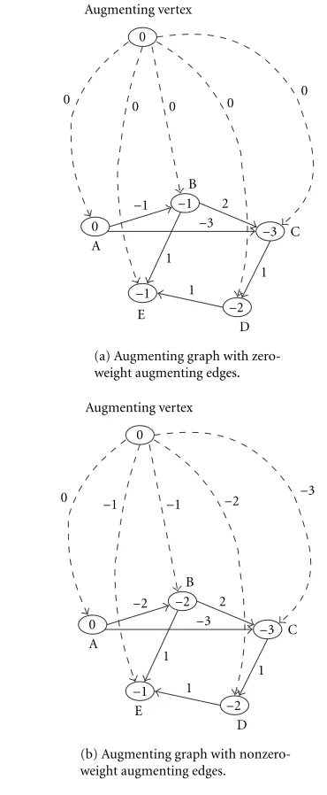
In the adaptive version of the algorithm, we are effectively setting the weights of the augmenting edges to be equal to the labels that were computed in the previous iteration. In this way, the initial scan from the augmenting vertex sets the dis-tance label at each vertex equal to the previously computed weight instead of setting it to 0. So we now need to show that using nonzero weights on the augmenting edges does not change the solution space in any way: that is, all possible solutions for the zero-weight problem are also solutions for the nonzero-weight problem, except possibly for translation by a constant.
The new algorithm with the adaptation enhancements can be seen to be correct if we relax the definition of the aug-mented graph so that the augmenting edges (froms0) need
not have zero-weight. We summarize the arguments for this in the following theorems.
Theorem 3. Consider a constraint graph augmented with a source vertexs0, and edges from this vertex to every other
ver-texv, such that these augmenting edges have arbitrary weight
weight(s0→v). The associated system of constraints is
Proof. Clearly, since s0 does not have any in-edges, no
cy-cles can pass through it. So any cycy-cles, negative or otherwise, which are detected in the augmented graph, must have come from the original constraint graph, which in turn would happen only if the constraint system was inconsistent (by Theorem 1). Also, any inconsistency in the original system would manifest itself as a negative cycle in the constraint graph, and the above augmentation cannot remove any such cycle.
The following theorem establishes the validity of solu-tions computed by the ABF algorithm.
Theorem 4. If G is the augmented graph with arbitrary weights as defined above, andD(u) = distG(s0, u)(shortest
paths froms0), then
(1) Dis a solution toV, C; and
(2) any solution toV, Ccan be converted into a solution to the constraint system represented byGby adding a constant toD(u)for eachu∈V.
Proof. The first part is obvious, by the definition of shortest paths.
Now we need to show that by augmenting the graph with arbitrary weight edges, we do not prevent certain solutions from being found. To see this, first note that any solution to a difference constraint system remains a solution when trans-lated by a constant. That is, we can add or subtract a constant to all theD(u) without changing the validity of the solution. In our case, if we have a solution to the constraint system that does not satisfy the constraints posed by our augmented graph, it is clear that the constraint violation can only be on one of the augmenting edges (since the underlying constraint graph is the same as in the case where the augmenting edges had zero weight). Therefore, if we define
lmax=max
weight(e)|e∈Sa, (3)
whereSais the set of augmenting edges and
D(u)=D(u)−l
max, (4)
we ensure thatDsatisfies all the constraints of the original graph, as well as all the constraints on the augmenting edges.
Theorem 4 tells us that an augmented constraint graph with arbitrary weights on the augmenting edges can also be used to find a feasible solution to a constraint system. This means that once we have found a solution dist : V → R (whereRis the set of real numbers) to the constraint system, we can change the augmented graph so that the weight on each edgee : u → vis dist(v). Now even if we change the underlying constraint graph in any way, we can use the same augmented graph to test the consistency of the new system.
Figure 1 helps to illustrate the concepts that are explained in the previous paragraphs. In Figure 1a, there is a change in the weight of one edge. But as we can see from the augmented graph, this will result in only the single update to the affected
D −2
1 1
E −1
1 −3
−3 C 2
−1 B −1 0 A
0
0 0 0 0 0
Augmenting vertex
(a) Augmenting graph with zero-weight augmenting edges.
D −2
1 1
E −1
1 −3
−3 C 2
−2 B −2 0 A
0
0 −1 −1 −2 −3
Augmenting vertex
(b) Augmenting graph with nonzero-weight augmenting edges.
Figure1: Constraint graph.
vertex itself, and all the other vertices will get their constraint satisfying values directly from the previous iteration.
In the example from Figure 1, the change in weight of edge AB means that after an initial scan to determine changes in distance labels, we find that vertex B is affected. However, on examining the outgoing edges from vertex B, we find that all other constraints are satisfied, so the Bellman-Ford al-gorithm can terminate here without proceeding to examine all other edges. Therefore, in this case, there is only 1 ver-tex whose label is affected out of the 5 vertices in the graph. Furthermore, the experiments show that even in large sparse graphs, the effect of any single change is usually localized to a small region of the graph, and this is the main reason that the adaptive approach is useful, as opposed to other techniques that are developed for more general graphs. Note that, as ex-plained in Section 2, the initial overhead for detecting con-straint violations still holds, but the complexity of this oper-ation is significantly less than that of the Bellman-Ford algo-rithm.
4. COMPARISON AGAINST OTHER INCREMENTAL ALGORITHMS
We compare the ABF algorithm against (a) the incremental algorithm developed in [4] for maintaining a solution to a set of difference constraints (referred to here as the RSJM algo-rithm), and (b) a modification of Howard’s algorithm [10], since it appears to be the fastest known algorithm to compute the cycle mean, and hence can also be used to check for fea-sibility of a system. Our modification allows us to use some of the properties of adaptation to reduce the computation in this algorithm.
The main idea of the adaptive algorithm is that it is used as a routine inside a loop corresponding to a larger pro-gram. As a result, in several applications where this negative cycle detection forms a computation bottleneck, there will be a proportional speedup in the overall application, which would be much larger than the speedup in a single run.
It is worth making a couple of observations at this point regarding the algorithms we compare against.
(1) The RSJM algorithm [4] uses Dijkstra’s algorithm as the core routine for quickly recomputing the shortest paths. Using the Bellman-Ford algorithm here (even with Tarjan’s implementation) would result in a loss in performance since it cannot match the performance of Dijkstra’s algorithm when edge weights are positive. Consequently, no benefit would be derived from the reduced-cost concept used in [4]. (2) The code for Howard’s algorithm was obtained from the Internet website of the authors of [10]. The modifica-tions suggested by Dasdan et al. [19] have been taken into account. This method of constraints checking uses Howard’s algorithm to see if the MCM of the system yields a feasible value, otherwise the system is deemed inconsistent.
Another important point is the type of graphs on which we have tested the algorithms. We have restricted our atten-tion tosparsegraphs, orbounded degreegraphs. In particular, we have tried to keep the vertex-to-edge ratio similar to what we may find in practice, as in, for example, the ISCAS bench-marks. To understand why such graphs are relevant, note the following two points about the structural elements
usu-ally found in circuits and signal processing blocks: (a) they typically have a small, finite number of inputs and outputs (e.g., AND gates, adders, etc. are binary elements) and (b) the fanout that is allowed in these systems is usually limited for reasons of signal strength preservation (buffers are used if necessary). For these reasons, the graphs representing prac-tical circuits can be well approximated by bounded degree graphs. In more general DSP application graphs, constraints such as fanout may be ignored, but the modular nature of these systems (they are built up of simpler, small modules) implies that they normally have small vertex degrees.
We have implemented all the algorithms under the LEDA [20] framework for uniformity. The tests were run on ran-dom graphs, with several ranran-dom variations performed on them thereafter. We kept the number of vertices constant and changed only the edges. This was done for the following rea-son: a change to a node (addition/deletion) may result in several edges being affected. In general, due to the random nature of the graph, we cannot know in advance the exact number of altered edges. Therefore, in order to keep track of the exact number of changes, we applied changes only to the edges. Note that when node changes are allowed, the argu-ment for an adaptive algorithm capable of handling multiple changes naturally becomes stronger.
In the discussion that follows, we use the termbatch-size
to refer to the number of changes in a multiple change up-date. That is, when we make multiple changes to a graph be-tween updates, the changes are treated as a single batch, and the actual number of changes that was made is referred to as the batch-size. This is a useful parameter to understand the performance of the algorithms.
The changes that were applied to the graph were of 3 types.
(i) Edge insertion: an edge is inserted into the graph, en-suring that multiple edges between vertices do not oc-cur.
(ii) Edge deletions: an edge is chosen at random and deleted from the graph. Note that, in general, this can-not cause any violations of constraints.
104
103
102
101
100
Batch size 10−2
10−1
100
101
102
103
Ru
n
ti
m
e
(s
)
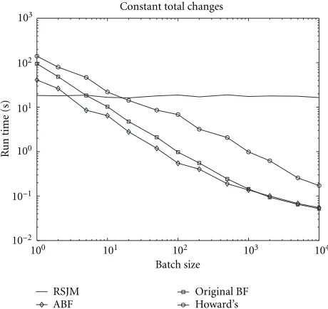
Constant total changes
RSJM ABF
Original BF Howard’s
Figure2: Comparison of algorithms as batch size varies.
10 9 8 7 6 5 4 3 2 1
Batch size 0
5 10 15 20 25 30 35
Ru
n
ti
m
e
(s
)
Varying batch size
RSJM ABF
Original BF Howard’s
Figure3: Constant number of iterations at different batch sizes.
performs most of the computation required to compute the maximum cycle mean of the graph, which is far more than necessary.
Figure 3 shows a plot of what happens when we apply 1000 batches of changes to the graph, but alter the number of changes per batch, so that the total number of changes ac-tually varies from 1000 to 100 000. As expected, RSJM takes total time proportional to the number of changes. But the other algorithms take nearly constant time as the batch size varies, which provides the benefit. The reason for the almost constant time seen here is that other bookkeeping operations dominate over the actual computation at this stage. As the
Table1: Relative speed of adaptiveversusincremental approach for graph of 1000 nodes, 2000 edges.
Batch size Speedup (RSJM time/ABF time)
1 0.26×
2 0.49×
5 1.23×
10 2.31×
20 4.44×
50 10.45×
100 18.61×
104
103
102
101
100
Batch size 10−1
100
101
102
103
Ru
n
ti
m
e
(s
)
Large batch effect (1000 nodes, 2000 edges)
RSJM ABF Original BF
Figure4: Asymptotic behavior of the algorithms.
batch size increases (asymptotically), we would expect that the adaptive algorithm takes more and more time to operate, finally converging to the same performance as the standard Bellman-Ford algorithm.
As mentioned previously, the adaptive algorithm is bet-ter than the incremental algorithm at handling changes in batches. Table 1 shows the relative speedup for different batch sizes on a graph of 1000 nodes and 2000 edges. Al-though the exact speedup may vary, it is clear that as the number of changes in a batch increases, the benefit of using the adaptive approach is considerable.
An important feature that can be noted from Figure 4 is the behavior of the algorithms as the number of changes between updates becomes very large. The RSJM algorithm is completely unaffected by this increase, since it has to continue processing changes one at a time. For very large changes, even when we start from scratch, we find that the total time for update starts to increase, because now the time taken to implement the changes itself becomes a factor that dominates overall performance. In between these two ex-tremes, we see that our incremental algorithm provides con-siderable improvements for small batch sizes, but for large batches of changes, it tends towards the performance of the original Bellman-Ford algorithm for negative cycle detection. From Figures 3 and 4, we see, as expected, that the RSJM algorithm takes time proportional to the total number of changes. Howard’s algorithm also appears to take more time when the number of changes increases. Figure 2 allows us to estimate at what batch size each of the other algorithms be-comes more efficient than the RSJM algorithm. Note that the scale on this figure is also logarithmic.
Another point to note with regard to these experiments is that they represent the relative behavior for graphs with 1000 vertices and 2000 edges. These numbers were chosen to obtain reasonable run times on the experiments. Similar re-sults are obtained for other graph sizes, with a slight trend in-dicating that thebreak-evenpoint, where our adaptive algo-rithm starts outperforming the incremental approach, shifts to lower batch-sizes for larger graphs.
5. APPLICATIONS
We present two applications that make extensive use of algo-rithms for negative cycle detection. In addition, these appli-cations also present situations where we encounter the same graph with slight modifications—either in the edge-weights (MCM computation) or in the actual addition and deletion of a small number of edges (scheduling search techniques). As a result, these provide good examples of the type of appli-cations that would benefit from the adaptive solution to the negative cycle detection problem. As mentioned in Section 1, these problems are central to the high-level synthesis of DSP systems.
5.1. Maximum cycle mean computation
The first application we consider is the computation of the MCM of a weighted digraph. This is defined as the maximum over all directed cycles of the sum of the arc weights divided by the number of delay elements on the arcs. This metric plays an important role in discrete systems and embedded systems [2, 21], since it represents the greatest throughput that can be extracted from the system. Also, as mentioned in [21], there are situations where it may be desirable to recom-pute this measure several times on closely related graphs, for example, for the purpose of design space exploration. As spe-cific examples, [6] proposes an algorithm for dataflow graph partitioning where the repeated computation of the MCM plays a key role, and [22] discusses the utility of frequent MCM computation to synchronization optimization in
em-bedded multiprocessors. Therefore, efficient algorithms for this problem can make it reasonable to consider using such solutions instead of the simpler heuristics that are otherwise necessary. Although several results such as [23, 24] provide polynomial time algorithms for the problem of MCM com-putation, the first extensive study of algorithmic alternatives for it has been undertaken by Dasdan et al. [2]. They con-cluded that the best existing algorithm in practice for this problem appears to be Howard’s algorithm, which, unfor-tunately, does not have a known polynomial bound on its running time.
To model this application, the edge weights on our graph are obtained from the equation
weight(u→v)=delay(e)×P−exec time(u), (5)
where weight(e) refers to the weight of the edgee :u →v, delay(e) refers to the number of delay elements (flip-flops) on the edge, exec time(u) is the propagation delay of the cir-cuit element that is the source of the vertex, andPis the de-sired clock period that we are testing the system for. In other words, if the graph with weights as mentioned above does not have negative cycles, thenPis a feasible clock for the system. We can then perform a binary search in order to compute P to any precision we require. This algorithm is attributed to Lawler [9]. Our contribution here is to apply the adaptive negative cycle detection techniques to this algorithm and an-alyze the improved algorithm that is obtained as a result.
5.1.1 Experimental setup
For an experimental study, we build on the work by Das-dan et al. [2], where the authors have conducted an exten-sive study of algorithms for this problem. They conclude that Howard’s algorithm [10] appears to be the fastest experimen-tally, even though no theoretical time bounds indicate this. As will be seen, our algorithm performs almost as well as Howard’s algorithm on several useful sized graphs, and espe-cially on the circuits of the ISCAS 89/93 benchmarks, where our algorithm typically performs better.
For comparison purposes, we implemented our algo-rithm in the C programming language, and compared it against the implementation provided by the authors of [10]. Although the authors do not claim their implementation is the fastest possible, it appears to be a very efficient imple-mentation, and we could not find any obvious ways of proving it. As we mentioned in the previous section, the im-plementation we used incorporates the improvements pro-posed by Dasdan et al. [2]. The experiments were run on a Sun Ultra SPARC-10 (333 MHz processor, 128 MB memory). This machine would classify as a medium-range workstation under present conditions.
One point to note is that since we are doing a binary search on T, we are forced to set a limit on the precision to which we compute our answer. This precision in turn de-pends on the maximum value of the edge-weights, as well as the actual precision desired in the application itself. Since these depend on the application, we have had to choose values for these. We have used a random graph generator that generates integer weights for the edges in the range [0– 10 000]. For this range of weights, it could be argued that in-teger precision would be sufficient. However, since the max-imum cycle mean is a ratio, it is not restricted to integer val-ues. We have therefore conservatively chosen a precision of 0.001 for the binary search (i.e., 10−7 times the maximum
edge-weight). Increasing the precision by a factor of 2 re-quires one more run of the negative cycle detection algo-rithm, which would imply a proportionate increase in the total time taken for computation of the MCM.
With regard to the ISCAS benchmarks, note that there is a slight ambiguity in translating the net-lists into graphs. This arises because aD-type flip-flop can either be treated as a single edge with a delay, with the fanout proceeding from the sink of this edge, or askseparate edges with unit delay emanating from the source vertex. In the former treatment, it makes more sense to talk about the|D|/|V|ratio (|D| be-ing the number ofDflip-flops), as opposed to the|D|/|E| ratio that we use in the experiments with random graphs. However, the difference between the two treatments is not significant and can be safely ignored.
We also conducted experiments where we vary the num-ber of edges with delays on them. For this, we need to ex-ercise care, since we may introduce cycles without delays on them, which are fundamentally infeasible and do not have a maximum cycle mean. To avoid this, we follow the policy of treating edges with delays as “back-edges” in an otherwise acyclic graph [15]. This view is inspired by the structure of circuits, where a delay element usually figures in the feed-back portion of the system. Unfortunately, one effect of this is that when we have a low number of delay edges, the result-ing graph tends to have an asymmetric structure: it is almost acyclic with only a few edges in the reverse “direction.” It is not clear how to get around this problem in a fashion that does not destroy the symmetry of the graph, since this re-quires solving thefeedback arc setproblem, which is NP-hard [25].
One effect of this is in the way it impacts the perfor-mance of the Bellman-Ford algorithm. When the number of edges with delays is small, there are several negative weight edges, which means that the standard Bellman-Ford algo-rithm spends large amounts of time trying to compute short-est paths initially. The incremental approach, however, is able to avoid this excess computation for large values ofT, which results in its performance being considerably faster when the number of delays is small.
Intuitively, therefore, for the above situation, we would expect our algorithm to perform better. This is because, for the MCM problem, a change in the value of P for which we are testing the system will cause changes in the weights of those edges which have delays on them. If these are
1 0.9 0.8 0.7 0.6 0.5 0.4 0.3 0.2 0.1 0
Feedback edge ratio 0
0.5 1 1.5 2 2.5 3 3.5 4 4.5 5
Ru
n
ti
m
e
(s
)
ABF-based MCM computation
MCM computation using normal BF routine Howard’s algorithm
Figure 5: Comparison of algorithms for 10 000 vertices, 20 000 edges: the number of feedback edges (with delays) is varied as a pro-portion of the total number of edges.
fewer, then we would expect that fewer operations would be required overall when we retain information across iter-ations. This is borne out by the experiments as discussed in Section 5.1.2.
Our experiments focus more on the kinds of graphs that appear to representrealgraphs. By this we mean graphs for which the average out-degree of a vertex (number of edges divided by number of vertices), and the relative number of edges with delays on them are similar to those found in real circuits. We have used the ISCAS benchmarks as a good rep-resentative sample of real circuits, and we can see that they show remarkable similarity in the parameters we have de-scribed: the average out-degree of a vertex is close to and a little less than 2, while an average of about (1/10)th or fewer edges have delays on them. An intuitive explanation for the former observation is that most real circuits are usually built up of a collection of simpler systems, which predomi-nantly have small numbers of inputs and outputs. For exam-ple, logic gates have typically 2 inputs and 1 output, as do elements such as adders and multipliers. More complex ele-ments like multiplexers and encoders are relatively rare, and even their effect is somewhat offset by input single-output units like NOT gates and filters.
5.1.2 Experimental results
We now present the results of the experiments on random graphs with different parameters of the graph being varied.
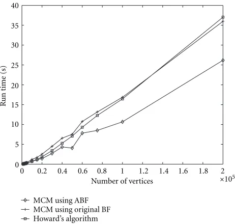
2
Figure 6: Performance of the algorithms as graph size varies: all edges have delays (feedback edges) and number of edges=twice the number of vertices.
the graph is nearly acyclic, and almost all edges have nega-tive weights. As a result, the normal Bellman-Ford algorithm performs a large number of computations that increase its running time. The ABF-based algorithm is able to avoid this overhead due to its property of retaining information across runs, and so it performs significantly better for small val-ues of the feedback edge ratio. The ABF-based algorithm and Howard’s algorithm perform almost identically in this exper-iment. The points on the plot represent an average over 10 random graphs each.
Figure 6 shows the effect of varying the number of ver-tices. The average degree of the graph is kept constant, so that there is an average of 2 edges per vertex, and the feed-back edge ratio is kept constant at 1 (all edges have delays). The reason for the choice of average degree was explained in Section 5.1.1. Figure 7 shows the same experiment, but this time with a feedback edge ratio of 0.1. We have limited the displayed portion of theY-axis since the values for the MCM computation using the original Bellman-Ford routine rise as high as 10 times that of the others and drowns them out oth-erwise.
These plots reveal an interesting point: as the size of the graph increases, Howard’s algorithm performs less well than the MCM computation using the ABF algorithm. This in-dicates that for real circuits, the ABF-based algorithm may actually be a better choice than Howard’s algorithm. This is borne out by the results of the ISCAS benchmarks.
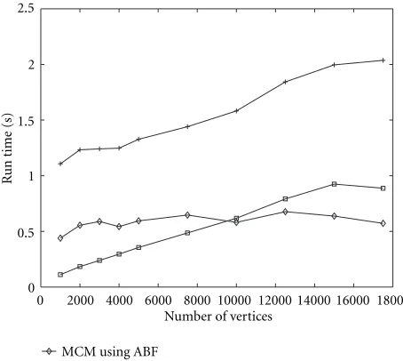
Figures 8 and 9 show a study of what happens as the edge-density of the graph is varied: for this, we have kept the num-ber of edges constant at 20 000, and the numnum-ber of vertices varies from 1000 to 17 500. This means a variation from an edge-density (ratio of the number of edges to the number of vertices) of 1.15 to 20. In both these figures, we see that
2
Figure7: Performance of the algorithms as graph size varies: pro-portion of edges with delays=0.1 and number of edges=twice the number of vertices (Y-axis limited to show detail).
18000
Figure 8: Performance of the algorithms as graph edge density varies: all edges have delays (feedback edges) and the number of edges=20 000.
18000 16000 14000 12000 10000 8000 6000 4000 2000 0
Number of vertices 0
0.5 1 1.5 2 2.5
Ru
n
ti
m
e
(s
)
MCM using ABF MCM using original BF Howard’s algorithm
Figure9: Performance of the algorithms as graph size varies: pro-portion of edges with delays= 0.1 and the number of edges=
20 000.
We note the following features from the experiments:
(i) If all edges have unit delay, the MCM algorithm that uses our adaptive negative cycle detection provides some benefit, but less than in the case where few edges have delays.
(ii) When we vary the number of feedback edges (edges with delays), the benefit of the modifications becomes very considerable at low feedback ratios, doing better than Howard’s algorithm for low-edge densities. (iii) In the ISCAS benchmarks, we can see that all of the
cir-cuits have|E|/|V|<2, and|D|/|V|<0.1, (|D|is the number of flip-flops,|V|is the total number of circuit elements, and|E|is the number of edges). In this range of parameters, our algorithm performs very well, even better than Howard’s algorithm in several cases (also see Table 2 for our results on the ISCAS benchmarks).
Table 2 shows the results obtained when we used the dif-ferent algorithms to compute MCMs for the circuits from the ISCAS 89/93 benchmark set. One point to note here is that the ISCAS circuits are not true HLS benchmarks; they were originally designed with logic circuits in mind, and as such, the normal assumption would be that all registers (flip-flops) in the system are triggered by the same clock. In order to use them for our testing, however, we have relaxed this as-sumption and allowed each flip-flop to be triggered on any phase; in particular, the phases that are computed by the MCM computation algorithm are such that the overall sys-tem speed is maximized. These benchmark circuits are still very important in the area of HLS, because real DSP circuits also show similar structure (sparseness and density of delay elements), and an important observation we can make from the experiments is that the structure of the graph is very
rel-Table2: Run time for MCM computation for the 6 largest ISCAS 89/93 benchmarks.
Bench- |E|/|V| |D|/|V| Orig. BF ABF Howard’s
mark MCM MCM algo.
s38417 1.416 0.069 2.71 0.29 0.66 s38584 1.665 0.069 2.66 0.63 0.59 s35932 1.701 0.097 1.79 0.37 0.09 s15850 1.380 0.057 1.47 0.18 0.36 s13207 1.382 0.077 0.73 0.12 0.35 s9234 1.408 0.039 0.57 0.06 0.11 s6669 1.657 0.070 0.74 0.07 0.04 s4863 1.688 0.042 0.27 0.04 0.03 s3330 1.541 0.067 0.11 0.02 0.01 s1423 1.662 0.099 0.07 0.01 0.01
evant to the performance of the various algorithms in the MCM computation.
As can be seen in Table 2, Lawler’s algorithm does reason-ably well at computing the MCM. However, when we use the adaptive negative cycle detection in place of the normal neg-ative cycle detection technique, there is an increase in speed by a factor of 5 to 10 in most cases. This increase in speed is in fact sufficient to make Lawler’s algorithm with this imple-mentation up to twice as fast as Howard’s algorithm, which was otherwise considered the fastest algorithm in practice for this problem.
5.2. Search techniques for scheduling
We demonstrate another application of our technique, effi -cient searching of schedules for IDFGs. The basic idea is that for scheduling an IDFG, we need to (a) assign vertices to pro-cessors and (b) assign relative positions to the vertices within each processor (for resource sharing). Once these two aspects are done, the schedule for a given throughput constraint is determined by finding a feasible solution to the constraint equations, which we do using the ABF algorithm. This idea that the ordering can be directly used to compute schedule times has been used previously, for example see [26]. Since the search process involves repeatedly checking the feasibil-ity of many similar constraint systems, the advantages of the adaptive negative cycle detection come into play.
The approach we have taken for the schedule search is
(i) start with each vertex on its own processor, find a fea-sible solution on the fastest posfea-sible processor; (ii) examine each vertex in turn, and try to find a place
for it on another processor (resource sharing). In do-ing so, we are makdo-ing a small number of changes to the constraint system, and need to recompute a feasi-ble solution;
(iii) in choosing the new position, choose one that has min-imum power (or area, or whatever cost we want to op-timize);
it as possible, moving vertices in groups from one pro-cessor to another, and so forth;
(v) the technique also lends itself very well to the applica-tion in schemes using evoluapplica-tionary improvement [27]; (vi) in the present implementation, to choose among var-ious equivalent implementations at a given stage, we use a weight based on giving greater importance to im-plementations that result in lower overall slack on the cycles in the system. (Slackof a cycle here refers to the difference between the total delay afforded by the reg-isters (number of delay elements in the cycle times the clock period) and the sum of the execution times of the vertices on the cycle, and is useful since a large slack could be taken as an indication of under-utilization of resources.)
Each such move or modification that we make to the graph can be treated as a set of edge-changes in the prece-dence/processor constraint graph, and a feasible schedule would be found if the system does not have negative cycles. In addition, the dist(v) values that are obtained from apply-ing the algorithm directly give us the startapply-ing times that will meet the schedule requirements.
We have applied this technique to attack the multiple-voltage scheduling problem addressed in [28]. The problem here is to find a schedule for the given DFG that minimizes the overall power consumption, subject to fixed constraints on the iteration period bound, and on the total number of resources available. For this example, we consider three re-sources: adders that operate at 5 V, adders that operate at 3.3 V, and multipliers that operate at 5 V. For the elliptic ter, multipliers operate in 2 time units, while for the FIR fil-ter, they operate in 1 time unit. The 5 V adders operate in 1 time unit, while the 3.3 V adders operate in 2 time units al-ways. It is clear that the power savings are obtained through scheduling as many adders as possible on 3.3 V adders in-stead of 5 V adders. We have used only the basic resource types mentioned in Table 3 to compare our results with those in [28]. However, there is no inherent limit imposed by the algorithm itself on the number of different kinds of resources that we can consider.
In tackling this problem, we have used only the most ba-sic method, namely, moving vertices onto another existing processor. Already, the results match and even outperform that obtained in [28]. In addition, the method has the ben-efit that it can handle any number of voltages/processors, and can also easily be extended to other problems, such as homogeneous-processor scheduling [15]. Table 3 shows the power savings that were obtained using this technique. S and R power saving indicates the power savings (assuming 25 units for 5 V devices and 10.89 units for 3.3 V devices) ob-tained by [28], while ABF power savings refers to the results obtained using our algorithm (where the ABF algorithm is used to test the feasibility of the system after eachmoveas per the definition above). The overall timing constraintTis the iteration period we are aiming for.
Table 3 shows some interesting features, the iterative im-provement based on the ABF algorithm (column marked
Table3: Comparison between the ABF-based search and algorithm of Sarrafzadeh and Raje [26] (×: failed to schedule,— : not avail-able).
Example Resource T Power saved (5 V+, 3.3 V+, 5 V∗) S and R ABF 5th order {2, 2, 2} 25 31.54% 34.86% ellip. filt. {2, 1, 2} 25 18.26% 16.60%
{2, 2, 2} 22 23.24% 26.56%
{2, 1, 2} 21 13.28% 14.94% FIR filt. {1, 2, 1} 15 29.45% ×
{1, 2, 2} 15 — 34.35%
{1, 2, 1} 16 — 36.81%
{1, 2, 2} 10 17.18% 24.54%
ABF) produced results with significantly higher power sav-ings than the results presented in [28]. One important reason contributing to this could be that the iterative improvement algorithm makes full use of the iterative nature of the graphs, and produces schedules that make good use of the available interiteration parallelism. On the other hand, we find that for one of the configurations, the ABF-based algorithm is not able to find any valid schedule. This is because the simple na-ture of the algorithm occasionally results in it getting stuck in local minima, with the result that it is unable to find a valid schedule even when one exists.
Several variations on this theme are possible; the search scheme could be used for other criteria such as the case where the architecture needs to be chosen (not fixed in advance), and modifications such as small amounts of randomization could be used to prevent the algorithm from getting stuck in local minima. This flexibility combined with the speed im-provements afforded by the improved adaptive negative cy-cle detection can allow this method to form the core of a large class of scheduling techniques.
6. CONCLUSIONS
The problem of negative cycle detection is considered in the context of HLS for DSP systems. It was shown that impor-tant problems such as performance analysis and design space exploration often result in the construction of “dynamic” graphs, where it is necessary to repeatedly perform negative cycle detection on variants of the original graph.
al-gorithm outperforms the incremental alal-gorithm (one change processed at a time) described in [4] even for changes made in groups of as little as 4–5 at a time.
As our original interest in the negative cycle detection problem arose from its application to the problems described above in HLS, we have implemented some schemes that make use of the adaptive approach to solve those problems. We have shown how our adaptive approach to negative cle detection can be exploited to compute the maximum cy-cle mean of a weighted digraph, which is a relevant metric for determining the throughput of DSP system implementa-tions. We have compared our ABF technique, and ABF-based MCM computation technique against the best known related work in the literature, and have observed favorable perfor-mance. Specifically, the new technique provides better per-formance than Howard’s algorithm for sparse graphs with relatively few edges that have delays.
Since computing power is cheaply available now, it is in-creasingly worthwhile to employ extensive search techniques for solving NP-hard analysis and design problems such as scheduling. The availability of an efficient adaptive nega-tive cycle detection algorithm can make this process much more efficient in many application contexts. We have demon-strated this concretely by employing our ABF algorithm within the framework of a search strategy for multiple volt-age scheduling.
ACKNOWLEDGMENTS
This research was supported in part by the US National Sci-ence Foundation (NSF) Grant #9734275, NSF NYI Award MIP9457397, and the Advanced Sensors Collaborative Tech-nology Alliance.
REFERENCES
[1] R. Reiter, “Scheduling parallel computations,” Journal of the ACM, vol. 15, no. 4, pp. 590–599, 1968.
[2] A. Dasdan, S. S. Irani, and R. K. Gupta, “Efficient algo-rithms for optimum cycle mean and optimum cost to time ratio problems,” in36th Design Automation Conference, pp. 37–42, New Orleans, La, USA, ACM/IEEE, June 1999. [3] B. Cherkassky and A. V. Goldberg, “Negative cycle detection
algorithms,” Tech. Rep. tr-96-029, NEC Research Institute, March 1996.
[4] G. Ramalingam, J. Song, L. Joskowicz, and R. E. Miller, “Solv-ing systems of difference constraints incrementally,” Algorith-mica, vol. 23, no. 3, pp. 261–275, 1999.
[5] D. Frigioni, A. Marchetti-Spaccamela, and U. Nanni, “Fully dynamic shortest paths and negative cycle detection on di-graphs with arbitrary arc weights,” in ESA ’98, vol. 1461 ofLecture Notes in Computer Science, pp. 320–331, Springer, Venice, Italy, August 1998.
[6] L.-T. Liu, M. Shih, J. Lillis, and C.-K. Cheng, “Data-flow par-titioning with clock period and latency constraints,” IEEE Trans. on Circuits and Systems I: Fundamental Theory and Ap-plications, vol. 44, no. 3, 1997.
[7] G. Ramalingam, Bounded incremental computation, Ph.D. thesis, University of Wisconsin, Madison, Wis, USA, August 1993, revised version published by Springer-Verlag (1996) as vol. 1089 ofLecture Notes in Computer Science.
[8] B. Alpern, R. Hoover, B. K. Rosen, P. F. Sweeney, and F. K. Zadeck, “Incremental evaluation of computational circuits,” in Proc. 1st ACM-SIAM Symposium on Discrete Algorithms, pp. 32–42, San Francisco, Calif, USA, January 1990.
[9] E. Lawler, Combinatorial Optimization: Networks and Ma-troids, Holt, Rhinehart and Winston, New York, NY, USA, 1976.
[10] J. Cochet-Terrasson, G. Cohen, S. Gaubert, M. McGettrick, and J.-P. Quadrat, “Numerical computation of spectral ele-ments in max-plus algebra,” inProc. IFAC Conf. on Syst. Struc-ture and Control, Nantes, France, July 1998.
[11] N. Chandrachoodan, S. S. Bhattacharyya, and K. J. R. Liu, “Adaptive negative cycle detection in dynamic graphs,” in
Proc. International Symposium on Circuits and Systems, vol. V, pp. 163–166, Sydney, Australia, May 2001.
[12] G. Ramalingam and T. Reps, “An incremental algorithm for a generalization of the shortest-paths problem,” Journal of Al-gorithms, vol. 21, no. 2, pp. 267–305, 1996.
[13] D. Frigioni, M. Ioffreda, U. Nanni, and G. Pasqualone, “Ex-perimental analysis of dynamic algorithms for single source shortest paths problem,” inProc. Workshop on Algorithm Engi-neering, pp. 54–63, Ca’ Dolfin, Venice, Italy, September 1997. [14] R. K. Ahuja, T. L. Magnanti, and J. B. Orlin, Network Flows,
Prentice-Hall, Upper Saddle River, NJ, USA, 1993.
[15] S. M. H. de Groot, S. H. Gerez, and O. E. Herrmann, “Range-chart-guided iterative data-flow graph scheduling,” IEEE Trans. on Circuits and Systems I: Fundamental Theory and Ap-plications, vol. 39, no. 5, pp. 351–364, 1992.
[16] K. K. Parhi and D. G. Messerschmitt, “Static rate-optimal scheduling of iterative data-flow programs via optimum un-folding,” IEEE Trans. on Computers, vol. 40, no. 2, pp. 178– 195, 1991.
[17] R. E. Tarjan, “Shortest paths,” Tech. Rep., AT&T Bell labora-tories, Murray Hill, New Jersey, USA, 1981.
[18] T. H. Cormen, C. E. Leiserson, and R. L. Rivest, Introduction to Algorithms, MIT Press, Cambridge, Mass, USA, 1990. [19] A. Dasdan, S. S. Irani, and R. K. Gupta, “An experimental
study of minimum mean cycle algorithms,” Tech. Rep. UCI-ICS #98-32, University of California, Irvine, 1998.
[20] K. Mehlhorn and S. N¨aher, “LEDA: A platform for combi-natorial and geometric computing,” Communications of the ACM, vol. 38, no. 1, pp. 96–102, 1995.
[21] K. Ito and K. K. Parhi, “Determining the minimum iteration period of an algorithm,”Journal of VLSI Signal Processing, vol. 11, no. 3, pp. 229–244, 1995.
[22] S. S. Bhattacharyya, S. Sriram, and E. A. Lee, “Resynchroniza-tion for multiprocessor DSP systems,”IEEE Trans. on Circuits and Systems I: Fundamental Theory and Applications, vol. 47, no. 11, pp. 1597–1609, 2000.
[23] D. Y. Chao and D. T. Wang, “Iteration bounds of single rate dataflow graphs for concurrent processing,” IEEE Trans. on Circuits and Systems I: Fundamental Theory and Applications, vol. 40, no. 9, pp. 629–634, 1993.
[24] S. H. Gerez, S. M. H. de Groot, and O. E. Hermann, “A poly-nomial time algorithm for computation of the iteration pe-riod bound in recursive dataflow graphs,”IEEE Trans. on Cir-cuits and Systems I: Fundamental Theory and Applications, vol. 39, no. 1, pp. 49–52, 1992.
[25] M. R. Garey and D. S. Johnson, Computers and Intractability—A Guide to the Theory of NP-Completeness, W. H. Freeman and Company, New York, NY, USA, 1979. [26] D. J. Wang and Y. H. Hu, “Fully static multiprocessor array
realizability criteria for real-time recurrent DSP applications,”
[27] T. B¨ack, U. Hammel, and H.-P. Schwefel, “Evolutionary com-putation: Comments on the history and current state,” IEEE Trans. Evolutionary Computation, vol. 1, no. 1, pp. 3–17, 1997. [28] M. Sarrafzadeh and S. Raje, “Scheduling with multiple volt-ages under resource constraints,” inProc. 1999 International Symposium on Circuits and Systems, pp. 350–353, Miami, Fla, USA, 30 May–2 June 1999.
Nitin Chandrachoodanwas born on Au-gust 11, 1975 in Madras, India. He received the B.Tech. degree in electronics and com-munications engineering from the Indian Institute of Technology, Madras, in 1996, and the M.S. degree in electrical engineer-ing from the University of Maryland at Col-lege Park in 1998. He is currently a Ph.D. candidate at the University of Maryland.
His research concerns analysis and representation techniques for system level synthesis of DSP dataflow graphs.
Shuvra S. Bhattacharyyareceived the B.S. degree from the University of Wisconsin at Madison, and the Ph.D. degree from the University of California at Berkeley. He is an Associate Professor in the Department of Electrical and Computer Engineering, and the Institute for Advanced Computer Stud-ies (UMIACS) at the University of Mary-land, College Park. He is also an Affiliate Associate Professor in the Department of
Computer Science. The coauthor of two books and the author or coauthor of more than 50 refereed technical articles, Dr. Bhat-tacharyya is a recipient of the NSF Career Award. His research in-terests center around architectures and computer-aided design for embedded systems, with emphasis on hardware/software codesign for signal, image, and video processing. Dr. Bhattacharyya has held industrial positions as a Researcher at Hitachi, and as a Compiler Developer at Kuck & Associates.
K. J. Ray Liureceived the B.S. degree from the National Taiwan University, and the Ph.D. degree from UCLA, both in electrical engineering. He is Professor at the Electri-cal and Computer Engineering Department of University of Maryland, College Park. His research interests span broad aspects of signal processing architectures; multime-dia communications and signal processing; wireless communications and networking;
information security; and bioinformatics in which he has pub-lished over 230 refereed papers, of which over 70 are in archival journals. Dr. Liu is the recipient of numerous awards including the 1994 National Science Foundation Young Investigator, the IEEE Signal Processing Society’s 1993 Senior Award, IEEE 50th Vehicu-lar Technology Conference Best Paper Award, Amsterdam, 1999. He also received the George Corcoran Award in 1994 for outstand-ing contributions to electrical engineeroutstand-ing education and the Out-standing Systems Engineering Faculty Award in 1996 in the recog-nition of outstanding contributions in interdisciplinary research, both from the University of Maryland. Dr. Liu is Editor-in-Chief of EURASIP Journal on Applied Signal Processing, and has been an Associate Editor of IEEE Transactions on Signal Processing, a Guest Editor of special issues on Multimedia Signal Processing of
![Table 3: Comparison between the ABF-based search and algorithmof Sarrafzadeh and Raje [26] (×: failed to schedule,— : not avail-able).](https://thumb-us.123doks.com/thumbv2/123dok_us/889244.1106938/13.600.309.549.111.235/table-comparison-based-search-algorithmof-sarrafzadeh-failed-schedule.webp)