Automatic Hierarchical Color Image Classification
Jing Huang
Department of Computer Science, Cornell University, Ithaca, NY 14853, USA Email:[email protected]
S. Ravi Kumar
Department of Computer Science, Cornell University, Ithaca, NY 14853, USA Email:[email protected]
Ramin Zabih
Department of Computer Science, Cornell University, Ithaca, NY 14853, USA Email:[email protected]
Received 20 March 2002 and in revised form 6 November 2002
Organizing images into semantic categories can be extremely useful for content-based image retrieval and image annotation. Grouping images into semantic classes is a difficult problem, however. Image classification attempts to solve this hard problem by using low-level image features. In this paper, we propose a method for hierarchical classification of images via supervised learning. This scheme relies on using a good low-level feature and subsequently performing feature-space reconfiguration using singular value decomposition to reduce noise and dimensionality. We use the training data to obtain a hierarchical classification tree that can be used to categorize new images. Our experimental results suggest that this scheme not only performs better than standard nearest-neighbor techniques, but also has both storage and computational advantages.
Keywords and phrases:image classification, color correlogram, classification tree.
1. INTRODUCTION
The proliferation of the worldwide web has given easy ac-cess to an explosively growing volume of visual data. Unfor-tunately, this data on the web is both scattered and unstruc-tured, making search and retrieval of information difficult. Such requirements have created great demands for effective and flexible systems to manage digital images/videos (e.g., [1,2,3,4,5,6]). Large digital libraries, which are built by collecting resources from different sites [5,7,8], can make searching relatively easier.
Most of the above systems generate low-level image fea-tures such as color, texture, shape, motion, and so forth, for image indexing and retrieval. This is partly because low-level features (e.g., color histograms, texture patterns) can be computed automatically and efficiently. However, the seman-tics of images, with which users prefer most of their inter-action, are seldom captured by low-level features. Currently, there is no effective method to automatically generate good semantic features of an image. One common compromise is to obtain some semantic information through manual an-notations. Since visual data contains rich information, the manual annotation process may be subjective and inconsis-tent. In addition, it is difficult to capture the content of an
image using words, not to mention the tedious manual la-bor involved in such a process. Another recent innovative approach, taken by the IMKA system [6], utilizes a medi-anet framework which combines the low-level features and semantic concepts in the same network and supports per-ceptual and semantic relationships among concepts, as the wordnet does.
Image classification
Image classification attempts to classify images into seman-tic categories by using low-level image features, and there-fore, bridges the gap between high-level semantics and low-level features. The categorization of images into classes can be helpful both for semantic organizations of digital libraries and for obtaining automatic annotations of images.
Figure1: Sample images from various classes.
A common approach to image classification involves ad-dressing the following three issues: (i) how to represent an image, (ii) how to organize the data, and (iii) how to clas-sify an image. Acquiring “nice” features and carefully mod-eling, the feature data are vital steps in this approach. Com-mon features include color, texture, and shape information
of an image. Some also integrate visual information and text accompanying an image [3,5,9].
navigation through the database, (ii) efficient retrieval, and (iii) ergonomically friendly presentation of the database. For instance, webseek, a web image search engine [7], uses hier-archical semantic structure for collecting and searching im-ages from the web. The image categories and hierarchies are preset by human design. Such an approach were also taken by [10,11] with very limited categories.
Our approach
In this paper, we propose a new scheme for automatic hi-erarchical image classification. We assume that a training set of images with known class labels is available. We use an easy-to-compute low-level feature, banded color correl-ograms, which has been shown to be effective and efficient for content-based image retrieval [12]. Using banded color correlograms for the training images, we model the feature data usingsingular value decomposition(SVD) [13] and con-structing aclassification tree. Once the classification tree is obtained, any new image can be easily classified. Our recur-sive method for constructing the classification tree is sum-marized below.
At each level of the classification tree, we aim to choose the best modeling of the training data. We first eliminate the
noise (or irrelevant variations) from the feature vectors us-ing SVD (or two-mode factor analysis). This step not only reduces the dimensionality of the feature vectors but also re-arranges the feature space to reflect the major correlation patterns in the data and ignores the smaller, less important variations.1 Using this noise-tolerant SVD representation,
we next classify each image in the training data using the nearest-neighbor algorithm with the first neighbor (which is the image itself) dropped (this is similar to leave-one-out cross-validation scheme). Based on the performance of this classification, we then partition the set of classes into two subclasses such that the intra-subclass association is maxi-mized while simultaneously the inter-subclass disassociation is minimized. This is accomplished using normalized cuts
[15]. Finally, the subclasses and those training images that were correctly classified with respect to the subclasses are worked upon recursively to obtain a hierarchical classifica-tion tree, with the hope of improving the classificaclassifica-tion per-formance.
Notice that a different SVD representation is used at each level of the tree. This flexibility in our method gives us the freedom to choose the size of the SVD representation as de-manded by each level, which in turn is dictated by the char-acteristics of classes involved.
We test our method on 11 fairly representative classes of Corel images. These 11 image classes are aviation photogra-phy, British motor car collection, Canadian Rockies, cats and kittens, clouds, dolphins and whales, flowers, night scenes, spectacular waterfalls, sunsets around the world, and waves. These images contain a wide range of content (scenery, animals, objects, etc.) and colors.
1SVD has been successfully used in latent semantic indexing for docu-ment retrieval [14].
We test our scheme using banded color correlograms and color histograms as features and compare our method to the nearest-neighbors algorithm directly applied to both color features. Our results suggest that this hierarchical scheme is able to perform consistently better than the already effective nearest-neighbor algorithm (see [16]). The classification tree we obtain also conforms with the semantic content of the 11 classes. Our results also suggest that correlograms have more
latent semanticstructures (than histograms) that can be ex-tracted by SVD procedure.
Organization
The rest of the paper is organized as follows.Section 2briefly describes the previous work in automatic image classifica-tion. Section 3 contains a brief description of the banded color correlogram we use in our experiments;Section 4 out-lines how to use SVD to model feature vectors; andSection 5
describes our hierarchical classification method. Section 6
contains our experimental results and Section 7concludes our discussions.
2. RELATED WORK
Since classification itself is a long-studied research area, dif-ferent classifiers can be tried on image classification (e.g.,
k-nearest neighbor, decision trees, Bayesian nets, maximum likelihood (ML) analysis, maximum a posterior (MAP) anal-ysis, linear discriminant analanal-ysis, neural networks, etc.). Not much work has been done on how to organize or select fea-tures. In the following, we review some previous work in im-age classification.
Vailaya et al. [11] use block image features and binary MAP classifier. An Image is first divided into blocks, and fea-tures are extracted from individual blocks. A few codebook vectors are used to estimate the class-dependent Gaussian mixture densities of the observed features. The image classes are organized by the following predefined hierarchical cate-gories: the first level is indoor/outdoor; the second level for outdoor images is city/landscape; the third level for land-scape images is sunset/mountain-forest; and the last one is to classify mountain/forest. These hierarchical five classes are fairly distinguishable from one another in terms of color and texture compared to the eleven classes inFigure 1, which are used for our test data. The binary classification at each level is over 90%. If the error propagation is included, the average classification accuracy of the five classes is degraded to 84%.
that take account of spatial information. Degrees of natural-ness, verticalnatural-ness, and openness are used to classify city cen-ters, skyscape, mountain, and beach scenes.
Carson et al. [16] propose a new representation for im-ages. Each image is thought to consist of severalblobs; each blob is coherent in color and texture space.2 All the blobs
in the training data of 14 image categories are clustered into about 180 “canonical” blobs using Gaussian models with di-agonal covariance. Each image is then assigned a score vec-tor which measures the nearest distance from each canoni-cal blob to the image. These score vectors are used to train a decision-tree classifier. The results of this method are com-pared to color histograms with the decision-tree classifier. In-terestingly, the color histograms seem to perform better than blobs.3
All the above works have only focused on visual fea-tures. Gevers et al. [10] try to integrate visual and textual features for web image classification. The textual informa-tion extracted from HTML tags is not always helpful for classification. For example, experiments of classifying im-ages into portraits/nonportraits show that the textual infor-mation does not help much. This is due to the inconsis-tent textual descriptions. In the case of classifying photo-graphic/synthetic images, the visual and textual features con-tribute equally to the classification. Hence, the composite features achieve better accuracy for this task. Paek et al. [9] also integrate visual and textual features for photograph clas-sification. Text is extracted from accompanying text of im-ages contained in news articles. The standard TF*IDF vectors are generated from text information, and a parallel OF*IIF vectors are produced from visual information. The OF*IIF vectors are supposed to be based on objects (which are par-allel to words) in images although the real implementation in [9] used cluster centroids of 8×8 image blocks. The in-tegrated vectors improves over the individual ones by about 3% in performance of an indoor/outdoor classification.
3. BANDED COLOR CORRELOGRAMS
In this section, we briefly review the banded color correlo-grams that we use in our experiments.
If we treat the color histogram as a probability distribu-tion of colors in an image, we ask the following quesdistribu-tion: pick any pixel p1of the imageᏵat distancekaway fromp1, pick
another pixelp2, what is the probability thatp2has the same
color asp1? The answer gives us the conditional probability
distribution that depicts the spatial correlation between the same color pixels. The color correlogram describes how this spatial correlation of colors changes with distances. We give the formal definitions below.
LetIbe ann1×n2image. The colors inIare quantized
intomcolorsc1, . . . , cm. For a pixelp = (x, y)∈ I, letI(p)
denote its color. LetIc= {∆ p|I(p)=c}. Thus, the notation
2This is one kind of color- and texture-based image segmentation me-thod.
3Several explanations were given for this performance degradation.
p∈Icis synonymous withp∈I,I(p)=c. For convenience, we use theL∞-norm to measure the distance between pixels,
that is, for pixels p1 =(x1, y1) and p2 =(x2, y2), we define
|p1−p2| =∆ max{|x1−x2|,|y1−y2|}. We denote the set
{1,2, . . . , n}by [n]. The size ofIis denoted by|I| =n1n2.
Histogram
Thecolor histogram(henceforth histogram)hofIis defined fori∈[m] by ability that a pixel at a distance k from the given pixel has the same color of p. (The factor 8kis due to the properties ofL∞-norm used to compute the distance between pixels.)
Note that the size of the autocorrelogram ismd. Since local correlations between colors are more significant than global correlations in an image, a small value of dis sufficient to
capture the spatial correlation.
We now define thebanded autocorrelogramas
βci(I)
This measure computes the localdensityof colorci’s correla-tion with itself, thus suggesting one kind of a local structure of colors. Note that the size of banded autocorrelogram ism, that is, the same as that of histogram. We useβ(I) to denote the banded autocorrelogram ofI, treated as vectors in anm -dimensional space.
We use theL1 (or the city-block) distance measure for
comparing histograms and banded autocorrelograms be-cause it is simple and robust. For simplicity, we will address banded autocorrelograms merely as correlograms for the re-mainder of the paper.
4. SINGULAR VALUE DECOMPOSITION
In this section, we briefly review the SVD that we use for or-ganizing image feature vectors.
Without loss of generality, letm≥n. For anm×nmatrix
(i) Uis anm×nmatrix, andΣ, Varen×nmatrices; (ii) U andV are column orthonormal, that is,UTU =
VTV =In;
(iii) Σ= diag(σ1, . . . , σr,0, . . . ,0), wherer = rank(A) and thesingular valuesareσ1≥σ2· · · ≥σr>0.
The first r columns of U and V together with the nonzero singular values actually are the eigenvectors and the
rnonzero eigenvalues ofAAT andATA, respectively. Several efficient algorithms exist to compute the SVD of a matrix, especially if the matrix is known to be sparse.
The SVD of a matrix can be used to obtain lower-rank approximations of the matrix. If we take the firstkcolumns ofUandV(denoted byU[k]andV[k]) and the leadingk×k
thenAkis the best rankkapproximation ofA, that is,
min
rank(B)=k|A−B|2=
A−Ak
2=σk+1. (5)
This property of the SVD helps to obtain a good trade-off between the quality of approximation and the size of the ap-proximation (i.e.,k). (To computeAk, we use the MATLAB built-in function SVD.)
The advantages of SVD are nicely exploited inlatent se-mantic indexing(LSI) for document retrieval [14]. The SVD, in some sense, derives the underlying structure that is hidden inA. The approximationAkcan be thought of as dampening the noise and that is present in the original matrixA. When SVD is applied to feature vectors, it not only eliminates the noise in the feature vectors but also reduces the dimension of the feature whenk < m.
We outline our approach of using SVD with correlo-grams. LetᏵ= {I1, . . . , In}denote the set of training images and letmbe the number of color quantizations. We define the matrixAi, j(Ᏽ)=∆ βci(Ij). We compute the SVD ofA(Ᏽ) to beA(Ᏽ)=UDVT. LetA
k =U[k]Σ[k]V[Tk]be an
approxi-mation toA. We can chooseU[k]as the basis for the newk
-dimensional feature space. Then,V[k]is the new
representa-tion for the correlograms in this reduced feature space. When we have a new image that needs to be classified, we first com-pute its correlogramq, then projectqonto the reduced fea-ture space by computing
q=q·U[k]·Σ−[k1]. (6)
Now, the question is how to choosekfor the approximation. We use the following heuristic to pick the k. Note that we want to find the best approximationAk such that the SVD representation of correlograms gives the best classification results using nearest-neighbor rule. Instead, we compute the classification for eachkbetween the number of classes (i.e.,c) to an upper limitk∗and choose the bestkin this range. Now, we show how to choosek∗. Notice that the singular values of
Acorrespond to the eigenvalues ofAAT, which is the corre-lation matrix of local color density for the training images. We setk∗to be thek∗th biggest eigenvalue within 2% of the maximum eigenvalue, that is, we ignore those correlations whose values are less than 2% of the maximum correlation.4
Note that, in the above SVD method, histograms can be used instead of correlograms. We will see (Section 6) that the performance with correlograms is much better than with histograms.
5. THE HIERARCHICAL CLASSIFICATION SCHEME
Image classificationis the problem of classifying images into known semantic classes. LetᏯ= {C1, . . . , Cc}be the image classes known as a priori. We assume that we have a set of training images whose class membership is known and we set᐀of images that need to be classified. We want to build a classification tree from training images. At each level of the classification tree, we aim to choose the best modeling of the training data. We first use SVD to eliminate the noise from the training data as described in Section 4. We then classify each image in the training data using the nearest-neighbor algorithm with the first nearest-neighbor dropped (similar to the leave-one-out cross-validation scheme). Based on the performance of this classification, we then split the classes into two subclasses such that the intra-subclass association is maximized while simultaneously the inter-subclass disasso-ciation is minimized. This is accomplished using normalized cuts [15]. Finally, the subclasses and those training images that were correctly classified with respect to the subclasses are worked upon recursively to obtain the hierarchy in the clas-sification tree, with the hope of improving the clasclas-sification performance.
5.1. Confusion matrix
We construct the matrixA() as indicated inSection 4and compute its SVD:A()=UΣVT. Then, we choose the best approximation Ak that gives the best classification ofon itself. The details are the following.
For an imageI ∈, andC(I) is the class ofI, letβk(I) denote thek-dimensional reduced SVD representation ofI. We consider eachI∈as a query and obtain the classC(I), neighbor classification when all images other thanIitself are considered. Intuitively, this procedure helps to find the best association patterns between the classes of SVD.
Now, thec×cconfusion matrixMis then defined by
Mi, j =size of
I|C(I)=Ci, C(I)=Cj
. (8)
The diagonal entries ofMare the number of images that are correctly classified, while the off-diagonal entries are the mis-classifications. The average percentage of correct classifica-tion is just the sum of the diagonal entries (trace (M)) di-vided by the size of.
5.2. Normalized cuts
We now show how to partition the confusion matrixM on the basis of maximizing the interclass association and mini-mizing the intraclass disassociation simultaneously. First, we review some basic definitions from graph theory.
Given a weighted graphG = V, Ewithw(u, v), being
is minimized. Mincuts can be computed in polynomial time using network flow techniques.
The confusion matrixMdefines a natural directed graph. The mincut in this graph corresponds to a partition of the classes intoM1andM2such that the number of
misclassifi-cations among these classes is minimized. A partition ofM
according to the mincut, however, sometime favors cutting small sets [20], that is, one ofV1 orV2 is very small. This
problem is considered in [15], where normalized cuts are in-troduced.
Formally, the normalized cut is given by the best partition ofV=V1∪V2that minimizes
The partition based on normalized cut is shown to have the property that minimizes the disassociation between the groups and maximizes the association within the group.
Define the diagonal matrixMi,i =
jMi, j. Normalized cuts can be computed reasonably well and efficiently by com-puting the second smallest eigenvalue of the system defined by (M−M)x=λMxand using some additional heuristics. The details can be looked up in [15].
We use normalized cuts to partitionMintoM1andM2,
accordingly, we obtain a partition of the classesᏯinto Ꮿ1
andᏯ2.
5.3. Classification tree
Using the normalized cuts, we can build the classification tree recursively. Given the original set of classesᏯ, we com-pute the partitionᏯ= Ꮿ1∪Ꮿ2based on normalized cuts.
We define1 = {I ∈ | C(I) ∈ Ꮿ1, C(I) ∈ Ꮿ1}and
2 = {I ∈ | C(I)∈ Ꮿ2, C(I)∈ Ꮿ2}. In this way, the
images that are misclassified across1and2are not
con-sidered from now on. We then recursively work on classifying
1(resp.,2) withᏯ1(resp.,Ꮿ2) as the set of classes (see [21]
Figure2: The classification tree obtained from the first training set using correlograms. The dotted lines indicate the trimmed portions.
5.4. Trimming
Sometimes, the performance of the classification on the training data does not always improve level by level using re-duced SVD representations. This is because some variations that are important to a set of classes may be removed by the SVD reduction. In this case, it does not pay offto recursively split such classes. Notice that this scenario can be detected automatically by comparing the performance of the tree be-fore and after trimming on the training set. More precisely, we perform a trimming procedure on the tree we obtain from the algorithm in the following manner: if the classification correctness of a node in the tree is higher than that of its two children, then we trim both the children; otherwise we keep the child with the higher correctness than the node itself and trim the other child. For instance,Figure 2shows a classifica-tion tree (corresponding to our sample set) with the trimmed portions marked.
6. EXPERIMENTS AND RESULTS
6.1. Experiments
images and test images are more or less the same. Therefore, we randomly shuffle the images in each class and take 70 im-ages as the training set and the rest 20 imim-ages as the test set. By doing so three times (to ensure fairness), we obtain three sets of training data and test data.
To compute color histograms and color correlograms, we quantize the RGB color space into 8×8×8 = 512 colors (3 bits for each color channel).5This level of quantization is
good enough for the SVD to extract the underlying structure, while not being too big (unlike 6912 colors used in [16]) so as to affect efficiency.
6.2. Results
We test both color correlograms and color histograms on the hierarchical classification approach and compare the hierar-chical approach with the nearest-neighbor classification. The three classification trees from three training sets are more or less the same and are consistent with the color content of the 11 classes. We only present the tree from the first data set (Figure 2). For the sake of simplicity, we abbreviate the names for the 11 classes: aviation (A1), British motors (B1), Canadian Rockies (C1), cats and kittens (C2), clouds (C3), dolphins and whales (D1), flowers (F1), night scenes (N1), spectacular waterfalls (S1), sunsets around the world (S2), and waves (W1). From the classification tree, we see that A1 and C3 share the same parent because of the same sky back-ground; similarly, W1, S1, and D1 are grouped together be-cause of the same water background.
The confusion matrices for different methods are shown in Table 1,Table 2, andTable 3. The classification behavior of the classification tree is quite different from the neighbor. The classification tree is better than the nearest-neighbor in that (i) the overall number of misclassifications between classes is smaller and (ii) the overall number of cor-rect classifications is larger.
The average percentage of correctness of the three test sets is summarized in Table 4. With correlograms and the classification-tree scheme, the average accuracy of classify-ing 11 image classes is about 82%, comparable to the 84% accuracy in [11] for a hierarchy of 5 image classes.6The
re-sults show that the hierarchical method is consistently better than the nearest-neighbor classification, and the color correl-ogram is consistently better than the color histcorrel-ogram.
Using the simple nearest-neighbor (NN) classification, the correlogram performs 3% better than the histogram; using the classification tree (CT), the correlogram performs 21% better than the histogram. Using the classification tree, the correlogram improves 3% over the nearest-neighbor; it improves 7% over the nearest-neighbor on the histogram. Note that the average data size of the SVD representations is about fifteen, 3% of the original size. The average number of nonleaf nodes in the classification trees is five after trimming.
5We also tried the HSV color space. The results do not change much. 6It is not meant to compare numbers here because the data set are diff er-ent.
Table 1: Class-confusion matrix for trimmed classification tree (correlogram).
A1 C3 C1 D1 W1 B1 C2 S1 F1 N1 S2
A1 17 0 0 3 0 0 0 0 0 0 0
C3 2 15 0 0 0 0 2 0 0 0 1
C1 0 2 16 2 0 0 0 0 0 0 0
D1 0 1 0 17 0 0 1 1 0 0 0
W1 0 1 1 4 13 0 0 1 0 0 0
B1 0 0 0 0 0 20 0 0 0 0 0
C2 0 0 0 0 0 0 20 0 0 0 0
S1 0 1 0 2 0 0 0 17 0 0 0
F1 1 0 0 0 0 1 1 0 17 0 0
N1 0 0 0 0 0 0 1 0 0 18 1
S2 0 0 0 0 0 1 0 0 2 0 17
Table2: Class-confusion matrix for the nearest-neighbor classifi-cation (correlogram).
A1 C3 C1 D1 W1 B1 C2 S1 F1 N1 S2
A1 16 1 0 2 0 0 1 0 0 0 0
C3 1 14 0 0 0 0 1 2 0 0 1
C1 0 0 15 5 0 0 0 0 0 0 0
D1 0 1 0 19 0 0 0 0 0 0 0
W1 0 0 0 2 17 0 0 1 0 0 0
B1 0 0 0 0 0 14 4 2 0 0 0
C2 0 0 0 0 0 0 20 0 0 0 0
S1 0 1 0 2 1 0 0 16 0 0 0
F1 1 0 0 0 0 0 2 0 14 1 2
N1 0 0 0 0 0 0 1 0 0 19 1
S2 0 2 0 0 0 0 0 0 0 2 16
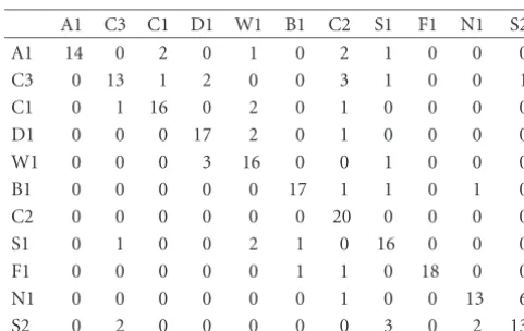
Table3: Class-confusion matrix for the nearest-neighbor classifi-cation (histogram).
A1 C3 C1 D1 W1 B1 C2 S1 F1 N1 S2
A1 14 0 2 0 1 0 2 1 0 0 0
C3 0 13 1 2 0 0 3 1 0 0 1
C1 0 1 16 0 2 0 1 0 0 0 0
D1 0 0 0 17 2 0 1 0 0 0 0
W1 0 0 0 3 16 0 0 1 0 0 0
B1 0 0 0 0 0 17 1 1 0 1 0
C2 0 0 0 0 0 0 20 0 0 0 0
S1 0 1 0 0 2 1 0 16 0 0 0
F1 0 0 0 0 0 1 1 0 18 0 0
N1 0 0 0 0 0 0 1 0 0 13 6
S2 0 2 0 0 0 0 0 3 0 2 13
Table4: Correctness classification on three data sets.
NN CT(Trim)
1 2 3 1 2 3
Hist. 0.786 0.746 0.786 0.696 0.677 0.668 Corr. 0.818 0.800 0.786 0.850 0.805 0.823
Remark6.1. We notice from the results that the color his-togram performs consistently worse with the classification tree than with the nearest-neighbor, while the color correlo-gram performs consistently better with the classification tree than with the nearest-neighbor. This suggests that correlo-grams have an underlying latent semantic structure (local color density). Color histograms do not seem to have such a property.
7. CONCLUSIONS AND FUTURE WORK
In this paper, we propose a hierarchical image tion method based on an automatic constructed classifica-tion tree. We use banded color correlograms as visual fea-tures and the SVD on the correlograms to extract a latent semantic structure of images for classification into semantic categories. SVD not only reduces the dimensionality of fea-tures but also removes the noise in the data. At each level of the classification tree, SVD is used to best model the data in terms of lowest classification errors. The data of a nonleaf node is then divided by the normalized cuts, which maxi-mizes the intra-subclass variation while simultaneously min-imizes the inter-subclass variation, to obtain the best classifi-cation results.
Our tests on 11 classes of Corel natural scene images show that our method using this scheme and a classification tree not only performs better than the nearest-neighbor clas-sification but also saves much computation and data storage. In addition, the results also suggest that the correlogram is more suitable for the image classification task than the color histogram. It will be interesting to usefeature-weighting tech-niques [22] and textual information to further assist SVD to get latent semantic structures from training data. The inte-gration of visual and textual features in our framework needs to be studied.
ACKNOWLEDGMENT
This work was done when the first two authors were at Cor-nell University.
REFERENCES
[1] M. Flickner, H. Sawhney, W. Niblack, et al., “Query by image and video content,” The QBIC System, IEEE Computer, vol. 28, no. 9, pp. 23–32, 1995.
[2] A. P. Pentland, R. Picard, and S. Sclaroff, “Photobook: content-based manipulation of image databases,” Interna-tional Journal of Computer Vision, vol. 18, no. 3, pp. 233–254, 1996.
[3] J. R. Smith and S.-F. Chang, “Visually searching the web for content,”IEEE MultiMedia, vol. 4, no. 3, pp. 12–20, 1997. [4] S. Mehrotra, Y. Rui, M. Ortega, and T. S. Huang, “Supporting
content-based queries over images in MARS,” inProc. IEEE International Conference on Multimedia Computing and Sys-tems, pp. 632–633, Ottawa, Ontario, Canada, June 1997. [5] T. Gevers and A. Smeulders, “The PicToSeek WWW image
search systems,” inIEEE International Conference on Multi-media Computing and Systems, vol. 1, pp. 264–269, Florence, Italy, June 1999.
[6] A. B. Benitez, S.-F. Chang, and J. R. Smith, “IMKA: a multime-dia organization system combining perceptual and semantic knowledge,” inProc. ACM Multimedia, pp. 630–631, Ottawa, Ontario, Canada, 2001.
[7] S-F. Chang, J. R. Smith, M. Beigi, and A. Benitez, “Visual information retrieval from large distributed online reposito-ries,”Communications of the ACM, vol. 40, no. 12, pp. 63–67, 1997.
[8] S. Sclaroff, L. Taycher, and M. La Cascia, “ImageRover: a content-based image browser for the world wide web,” inProc. of IEEE Workshop on Content-Based Access of Image and Video Libraries, pp. 2–9, San Juan, PR, USA, June 1997.
[9] S. Paek, C. Sable, V. Hatzivassiloglou, et al., “Integration of visual and text-based approaches for the content labelling and classification of photographs,” inACM SIGIR ’99 Workshop on Multimedia Indexing and Retrieval, Berkeley, Calif, USA, August 1999.
[10] T. Gevers, F. Aldershoff, and A. Smeulders, “Classification of images on internet by visual and textual information,” in In-ternet Imaging, SPIE, San Jose, Calif, USA, January 2000. [11] A. Vailaya, M. Figueiredo, A. Jain, and H. J. Zhang, “Bayesian
framework for hierarchical semantic classification of vacation images,” IEEE Trans. on Image Processing, vol. 1, no. 1, pp. 117–130, 2001.
[12] J. Huang, S. R. Kumar, M. Mitra, and W. J. Zhu, “Spatial color indexing and applications,” inProc. of 8th International Conf. on Computer Vision, 1998.
[13] G. H. Golub and C. F. Van Loan, Matrix Computations, The Johns Hopkins University Press, Baltimore, Md, USA, 1989. [14] S. Deerwester, S. Dumais, G. Furnas, T. Landauer, and
R. Harshman, “Indexing by latent semantic analysis,” Jour-nal of the American Society of Information science, vol. 41, no. 6, pp. 391–407, 1990.
[15] J. Shi and J. Malik, “Normalized cuts and image segmenta-tion,” inProc. 16th IEEE Computer Society Conference on Com-puter Vision and Pattern Recognition, pp. 731–737, San Juan, PR, USA, June 1997.
[16] C. Carson, S. Belongie, H. Greenspan, and J. Malik, “Color-and texture-based image segmentation using EM “Color-and its ap-plication to image querying and classification,” submitted to IEEE Trans. on Pattern Analysis and Machine Intelligence. [17] P. Lipson, E. Grimson, and P. Sinha, “Configuration based
scene classification and image indexing,” inProc. 16th IEEE Conf. on Computer Vision and Pattern Recognition, pp. 1007– 1013, San Juan, PR, USA, June 1997.
[18] A. Torralba and A. Oliva, “Semantic organization of scenes us-ing discriminant structural templates,” inProc. International Conf. on Computer Vision, pp. 1253–1258, Corfu, Greece, 1999.
[19] H. Borko and M. Bernick, “Automatic document classifica-tion,”Journal of the ACM, vol. 9, pp. 512–521, 1962. [20] Z. Wu and R. Leahy, “An optimal graph theoretic approach to
[21] J. Huang,Color-spatial image indexing and applications, Ph.D. thesis, Dept. of Computer Science, Cornell University, Ithaca, NY, USA, 1998.
[22] D. Wettschereck, D. W. Aha, and T. Mohri, “A review and empirical evaluation of feature weighting methods for a class of lazy learning algorithms,”Artificial Intelligence Review, vol. 11, no. 1-5, pp. 273–314, 1997, Special issue on lazy learning algorithms.
Jing Huangis a research staffmember at IBM T. J. Watson Research Center. She re-ceived the B.S. and the M.S. degrees in ap-plied mathematics from Tsinghua Univer-sity, Beijing, China, and the Ph.D. in com-puter science from Cornell University. Her Ph.D. work focused on computer vision and content-based image retrieval. After join-ing the IBM T. J. Watson Research Center, she switched to work on automatic speech
recognition. Her research interest also includes machine learning and information extraction.
S. Ravi Kumaris a research staffmember at IBM Almaden Research Center. He re-ceived the B.S. degree in computer engi-neering from Anna University, Madias, dia, and the M.S. degree from Indian In-stitute of Science, Bangalore, India. He fin-ished his Ph.D. study in computer science from Cornell University in 1998. His Re-search includes theory of computation, es-pecially in randomization, complexity the-ory, and web algorithms.