Cluster Structure Inference Based on Clustering Stability with Applications to Microarray Data Analysis

(1)

Cluster Structure Inference Based on Clustering

Stability with Applications to Microarray

Data Analysis

Ciprian Doru Giurc ˘aneanu

Institute of Signal Processing, Tampere University of Technology, P.O. Box 553, FIN-33101 Tampere, Finland Email:[email protected]

Ioan T ˘abus¸

Institute of Signal Processing, Tampere University of Technology, P.O. Box 553, FIN-33101 Tampere, Finland Email:[email protected]

Received 28 February 2003; Revised 7 July 2003

This paper focuses on the stability-based approach for estimating the number of clustersKin microarray data. The cluster stability approach amounts to performing clustering successively over random subsets of the available data and evaluating an index which expresses the similarity of the successive partitions obtained. We present a method for automatically estimatingKby starting from the distribution of the similarity index. We investigate how the selection of the hierarchical clustering (HC) method, respectively, the similarity index, influences the estimation accuracy. The paper introduces a new similarity index based on a partition distance. The performance of the new index and that of other well-known indices are experimentally evaluated by comparing the “true” data partition with the partition obtained at each level of an HC tree. A case study is conducted with a publicly available Leukemia dataset.

Keywords and phrases:clustering stability, number of clusters, hierarchical clustering methods, similarity indices, partition-distance, microarray data.

1. INTRODUCTION

The clustering algorithms are frequently used for analyzing the microarray data. While various clustering methods help the practitioner in bioinformatics to ascertain different char-acteristics in structural organization of microarray datasets, the task of selecting the most appropriate algorithm for solv-ing a particular problem is nontrivial. While various cluster-ing methods are applied in hundreds of microarray research papers, a question arises frequently, namely, how to compare two different partitions of the same dataset obtained by two different algorithms. The comparison becomes more difficult when the two partitions do not contain the same number of clusters. The accurate estimation for the number of clusters

K is essential because most of the existing clustering proce-dures requestKas input.

The robustness of the clustering algorithms is usually studied by investigating their stability with respect to pertur-bations changing the original dataset, for example, by draw-ing random subsets or by artificially adddraw-ing noise [1]. The stability methods can be also used in exploratory data

anal-ysis when little prior information is available regarding the dataset, which is generally the case with microarray data. The main principle is to randomly split the dataset and cluster each subset independently, and then to check the stability (or degree of agreement) of the two obtained partitions. The clustering is stable if the cluster memberships inferred in the two subsets are similar to the memberships in the entire sam-ple [1]. The following two diﬀerent approaches have been considered when applying the stability methods for finding structure in microarray data.

(1) After randomly splitting the dataset into two subsets, select one subset for learning and another for test. Firstly, a clustering algorithm CA is applied to the learning set, and the resulting classes are used to classify the samples which belong to the test set. Then the test set is clustered with the same algorithmCA, and a similarity measure (index) is com-puted between the labels produced by classification, respec-tively, clustering [2,3,4].

(2)

introduced in [6]:CAis applied to the whole dataset (refer-ence clustering) and to a randomly chosen subset. The sim-ilarity index is computed for the samples contained in the selected subset.

In both approaches, it is assumed that the number of clusters is k ∈ {2, 3,. . .,kmax}, and for each value allowed fork, after running the algorithm many times, the empir-ical distribution of the similarity index is collected. In [3], the number of clustersK is estimated based on the median of similarity index values. Evaluating the degree of agree-ment is rephrased in [4] as a prediction problem: their index (“prediction strength”) ps(k) measures how well the cluster centroids from the training set predict “co-memberships” in the test set. The index ps(k) is averaged over several ran-dom splittings of the original data (into training set and test set), and the estimated number of clusters is given by

ˆ

K =arg max2≤k≤kmaxmean[ps(k)] when max(mean[ps(k)]) is larger than a given threshold. The approach in [6] eval-uates the stability for individual patterns and clusters rely-ing on a diﬀerent similarity score called optimal association. In [5], ˆK is chosen as the value, where there is a transition from a similarity index distribution that is concentrated near one to a wider distribution: ˆKis visually estimated by using the empirical cumulative distribution function or, alterna-tively, based on the value of the 90th percentile. In consensus clustering (CC) [7], the central role is played by the consen-sus matrix that records, for every pair of objects, the pro-portion of clustering runs in which the two objects are clus-tered together. Based on the histogram of the consensus ma-trix entries, an empirical cumulative distribution function is defined, and the selection of the appropriate number of clus-ters proceeds by inspection of the shape of this function when

k∈ {2, 3,. . .,kmax}.

We propose to improve the algorithm described in [5] such that ˆKcan be automatically estimated without resort-ing to visual inspection or other heuristic methods. To eval-uate the importance of index selection on the accuracy of the estimation, we revisit various similarity indices. Then we de-fine and analyze a new similarity index, which is connected to the recently introduced partition distance [8]. In [3,5], the Fowlkes-Mallows index [9] is recommended for stability-based methods, but we show experimentally that our newly introduced index and the Jaccard index [10] perform better. We also show in this paper that partition distance is useful in designing a visualization tool which helps consistently the interpretation of clustering results for microarray data.

Potentially, any clustering algorithm can be used in our settings, and we investigate the impact of the algorithm selec-tion on the estimated ˆK. We restrict our investigation to the agglomerative hierarchical clustering (HC) algorithms [10] mainly because this class of clustering methods is very pop-ular in microarray data analysis [11]. These algorithms are computationally eﬃcient since the same tree can be used for all values of k ∈ {2, 3,. . .,kmax} by looking at diﬀ er-ent levels of the tree each time. In [7], when evaluating the performances of CC with various microarray datasets, it was concluded that CC based on HC produces slightly bet-ter results than CC based on self-organizing maps (SOM).

We remark that in [5,6,7] the HC is done by the group-average algorithm [10,12]. In our simulated experiments, the group-average shows modest results when compared with complete-linkage and Ward’s methods [10,12].

The remainder of this paper is organized as follows.

Section 2includes a discussion of some results on the esti-mation of the number of clusters, previously reported for the publicly available Leukemia dataset [13]. In Section 3, we introduce the similarity indices. Relying on the revisited properties of the partition distance [8], a new similarity in-dexs(·,·) is defined, and a lower bound is found under the hypothesis of generalized hypergeometric distribution for the contingency table. InSection 4, we evaluate experimen-tally s(·,·) by comparing the “true” clustering of a dataset with the partition obtained at each level of a HC tree. In

Section 5, we introduce the stability-based method for find-ing the data structure by extendfind-ing the approach proposed in [5]. Comparisons with other methods are reported for simu-lated data, and a case study is conducted on Leukemia dataset [13].

2. MOTIVATION OF THE WORK

In order to illustrate the challenge of structure estimation for microarray data, we consider the leukemia dataset de-scribed in [13], publicly available athttp://www-genome.wi. mit.edu/cgi-bin/cancer/datasets.cgi, which comes from a study of gene expression in two types of acute leukemias, acute lymphoblastic leukemia (ALL) and acute myeloid leukemia (AML). The true number of classes may be consid-ered three since the biological labeling of the patient samples is ALL-B, ALL-T, and AML [13]. The dataset consists of 6817 human genes measured for 72 patients: 47 cases of ALL (38 B-cell ALL and 9 T-cell ALL) and 25 cases of AML.

We note that the clustering of Leukemia dataset was al-ready investigated in several studies. In [13], the SOM are applied to cluster measurements from 38 patients (out of 72), relying on 50 “informative” genes selected based on a super-vised procedure. We emphasize here that the “informative” genes selection relies on the gene correlation with diﬀerent types of Leukemia. In two recent publications [14,15], var-ious validation techniques based on computing internal in-dices are used to estimate the number of clusters in the 38×50 dataset when SOM is the clustering algorithm. The paper [15] concludes that the estimated number of clusters is ˆK=2 and mentions, as a second best choice, ˆK=4.

The whole set of measurements from the 72 patients is clustered in [16] byk-means, fuzzyc-means networks, SOM, fuzzy SOM, and growing cell structure (GCS) algorithm. When varying the number of clusters between 2 and 16, all the resulting clusterings are evaluated based on the distribu-tion of Leukemia types within the clusters, the highest de-gree of intracluster homogeneity being obtained when sam-ples are divided into 9 clusters by fuzzy SOM. A procedure for gene selection is applied.

(3)

samples: for ˆK =3, one ALL B-cell sample is clustered with the ALL T-cell samples, and the rest of the observations are allocated correctly. Results on estimating the number of clus-ters are also reported: applyingclest,kl[17],hart[18], or sil-houtte (sil) [10] leads to ˆK = 3;ch[19] estimates ˆK = 2. The estimated number of clusters is ˆK=10 when usinggap

[20], and ˆK=5 when employinggapPC[20]. Note thatclest

was originally introduced in [3] and extends the stability-based approach from [2]. Another method relying on stabil-ity principle, CC, was formalized and tested in [7]. Since their settings allow to apply various clustering methods, results on estimated number of clusters for 38 (out of 72) samples of Leukemia dataset are reported when using HC and SOM. The method CC in conjunction with HC leads to ˆK=5, and to ˆK=4 when employing CC in combination with SOM.

In light of these results reported for the Leukemia dataset, we can better understand the importance and diﬃculty of validation of the number of clusters. It becomes apparent that every method for structure estimation must be deeply analyzed and validated with simulated data for which the true nature is known before applying it to analyze the mi-croarray data. Leukemia dataset is also a good example for illustrating the paradigm of “high dimension and small sam-ple size” which is common in microarray data analysis. It was pointed out in [7] that this paradigm prevents the use of some clustering algorithms, and we show in this paper how stability methods can circumvent this diﬃculty.

3. SIMILARITY MEASURES

Tcluster. So, any partition ofTis a set of mutually exclusive clusters whose reunion isT.

The partitionsP andP are identical if and only if ev-ery cluster in P is a cluster in P. LetM be an r×c ma-trix where the quantitymi jis the number of objects in com-mon between theith cluster ofPand the jth cluster ofP. The contingency table is represented inTable 1, wheremi·

c

j=1mi jfor 1≤i≤randm·j

r

i=1mi jfor 1≤j≤c. It is easy to observe thatm··ri=1mi·=cj=1m·j=N.

3.1. Rand, Jaccard, and Fowlkes-Mallows similarity indices

We introduce the following function relative to an arbitrary partitionPofT: for any pair of distinct objects (O,Om)∈

Table1: The contingency table for the partitionsPandP of the N-object setT.

which indicates if two objects belong to the same cluster in the partitionP.

Following a classic procedure, we firstly define four sets:

ᐃ1

and denote the cardinalities of these sets, wi |ᐃi| for

i∈ {1, 2, 3, 4}. Then we recall the definitions for three well-known similarity indices:

Sincewi(1≤i≤4) are nonnegative numbers, all three indices take values in the interval [0, 1]. The partitionsPand

P are identical if and only ifw2 = w3 =0; when they are identical andw1=0, then all indices are equal to their max-imum value 1. Observe for the denominator of Rand index that4i=1wi=

N 2

. The Jaccard index is not defined for the trivial case when each cluster inP andPcontains at most 1 object, which is equivalent to w1 = w2 = w3 = 0. The Fowlkes-Mallows index is not defined whenw1 = w2 = 0 (each cluster inPcontains at most 1 object) orw1=w3=0 (each cluster inPcontains at most 1 object). Formulae for fast computingwi(1≤i≤4) are available [23].

To each similarity measuresm(P,P), bounded by zero and unity, we can associate a dissimilarity d(P,P) 1−

sm(P,P); in some cases,d(P,P) could be a metric on the set of all partitions of a given set of objects T [12]. In the next section, we start from the definition given in [8] for the partition distance (which is a metric) and define a new simi-larity index.

3.2. A similarity index defined as complement of a partition distance

(4)

T, so that the two induced partitions (PandPrestricted to the remaining elements) are identical.” It was pointed out in [24] that the partition distance is also equal to the minimum number of elements that must be moved between clusters in

P, so that the resulting partition equalsP(with the conven-tion that any set which becomes empty is no longer a cluster).

Proposition 1. The partition distanceD(P,P)is a metric on the set of all partitions of a given set of objectsT.

Proof. SeeAppendix A.

Anassignmentis a selection of entries of the contingency matrixM such that no row or column contains more than one selected entry and is calledoptimalwhen the sum of the selected cell values is the largest over all possible assignments [24]. LetA(P,P) denote the value of the optimal assignment for the contingency matrixM.

Theorem 1 [24]. Two properties of partition distance:

(a)The relationship between the partition distance and the optimal assignment is given byD(P,P)=N−A(P,P).

(b)The elements to be removed fromTto induce identical partitions onPandP, are all those objects not associated with any selected cells of the optimal assignment.

The proof of the theorem is given in [24] where the theo-rem is further used to show how the partition distance can be computed in ᏻ((r +c)3_{) time after creating the matrix} M inᏻ(N) time. Note that the initial algorithm proposed in [8] to computeD(P,P) for any pair of partitions (P,P) is an exponential-time algorithm, and the algorithm in [24] reduces dramatically the computational complexity.

Proposition 2. The maximum of the partition distance is

max(P,P)D(P,P)=N−1and is achieved if and only if one

partition consists of a single cluster and the other one consists only of clusters containing single-objects.

Proof. SeeAppendix A.

The above results suggest the definition of the following index of similarity between any two partitionsPandP:

s(P,P)1−D(P,P)

N−1 =

A(P,P)−1

N−1 . (3)

The new index is a measure of similarity ranging from

s(P,P)=0 when the two partitions have no similarities (i.e., when one consists of a single cluster and the other only of clusters containing single-objects) tos(P,P) =1 when the partitions are identical.

Any injective mapping σ : {1, 2,. . .,|P|} → {1, 2,. . ., |P|}(|P| ≤ |P|) is called association [6] and is useful for comparing two partitionsPandPdefined over anNobject setT. The measure of similarity betweenPandPis com-puted as s∗(P,P) maxσ(·)(1/N)

_|P_|

j=1mσ(j),j wherem·,·

denotes the entries of the contingency matrix. Observe that

s∗(P,P)=A(P,P)/Nand is close to the similarity index de-fined in (3);A(P,P)≤Nimplies thats(P,P)≤s∗(P,P). It

Table2: The contingency table for the Leukemia dataset: the true partition given by a priori knowledge on the type of disease for each patient is compared with the partition produced by complete-linkage algorithm when ˆK=3. All the 3571 genes are used for clus-tering. The entries associated to the optimal assignment are repre-sented in bold.

Cluster ALL B-cell ALL T-cell AML

C1 26 8 8

C2 7 0 2

C3 5 1 15

is noticed in [6] that the computation ofs∗(P,P) by brute-force enumeration is exponential in the number of clusters, and therefore an approximative greedy heuristic was used there for finding a suboptimal associationσ(·). Since then, the fast algorithm was introduced in [24], and hence we are going to use the fast, nonapproximative evaluation of

s(P,P).

We observe that the definition of both s(P,P) and

s∗(P,P) relies on the optimal assignmentA(P,P), and the main diﬀerence between these similarity indices is given by the normalization procedure. Since in [6]s∗(P,P) was suc-cessfully applied for detecting stable clusters in microarray data, we are encouraged to employs(P,P) in stability-based methods for analyzing data produced by microarray tech-nology. The superiority of our approach consists in using nonapproximative algorithms for computing the similarity index.

The use ofs(·,·) in validation of microarray data clus-tering is appealing since the optimal assignment lends it-self to be employed as a visualization tool. Assume that we depict the contingency matrix defined by two partitions P

andP, whereP corresponds to the classes in a microarray dataset already known from medical evidence whileP con-tains classes found for the same dataset after running a clus-tering algorithm. Representing in bold the entries associated to the optimal assignment will allow the investigator to as-sess very easily the memberships. The procedure does not re-quire the number of clusters to be the same in the compared partitions. Moreover, the number of clusters can be visually assessed by checking that all entries in the optimal assign-ment are larger than zero. Examples of such representations are given inSection 5.2, Tables2and8. When the true state of the nature is not known, the same graphical representa-tion can be used for comparing the results of two diﬀerent clustering algorithms.

3.3. Similarity indices “corrected for chance”

A similarity index is “corrected for chance” when the expec-tation of the index takes some constant value (e.g., zero) un-der an appropriate null model for the contingency table. The property is discussed in [25], and the following general for-mula is proposed to correct an index:

Index−Expected Index

(5)

The most popular null model assumes that ther×c con-tingency table (r ≥ c) is constructed from the generalized hypergeometric distribution. The main hypothesis is that the two partitions are mutually independent and subject to the condition that the cluster sizes are fixed at (α1,α2,. . .,αr) and (β1,β2,. . .,βc), respectively. Theαiandβj are the marginal totals ofmi j, namely,mi·andm·j, respectively. Then the ex-pectation ofmi j isE[mi j] = αiβj/N [9,25]. For example, correcting the Rand index under this hypothesis leads to the expression

Adjusted Rand= w14+w4−Nc i=1wi−Nc

, (5)

where two diﬀerent formulae were proposed forNc in [25,

26]. We use in the sequel the notations RandHAand RandMA for the adjusted index defined in [25], respectively, [26].

We investigate in Appendix B the existence of a lower bound for the expectation of the similarity index defined by (3) when the hypothesis of generalized hypergeometric dis-tribution is verified.

It was already pointed out in [3] that the assumption on the statistical independence of the two compared clusterings does not hold for stability methods since the same data are used to produce both partitions. To gain more insights on the possibility of using s(·,·) in practical applications, we study inAppendix Cthe asymptotic and finite characteris-tics of s(·,·) and compare them with the characteristics of other similarity indices.

4. USING THE SIMILARITY INDEXs(·,·)IN HIERARCHICAL CLUSTER ANALYSIS

The aim of this section is to evaluate experimentally s(·,·) when we assume that the “true” structure of the data (the number of clusters and the membership) is known and com-pare this partition with the partition obtained at each level of a HC tree.

It is a well-known fact that the HC does not yield a dis-crete number of clusters, but rather a hierarchical arrange-ment between objects. For better understanding of the be-havior of similarity indices, assume that the “true” struc-ture of the data is known and compare this partition with the partition obtained at each level of the HC solution. This approach was originally used in [27] to compare Rand, RandHA, RandMA, Fowlkes-Mallows, and Jaccard indices.

We reconsider the experiments described in [27] to eval-uate the newly introduced indexs(·,·), and for comparison, we compute also Rand, RandHA, and Jaccard indices. For the first set of experiments, each generated dataset consists of 50 points uniformly distributed in a hypercube in 4-, 6-, or 8-dimensional Euclidean space. There is no significant cluster structure in the data, but a “criterion” solution is assumed: a hypothetical number of clusters (set at either 2, 3, 4, or 5) and a particular distribution pattern of the points to the clusters. Three density patterns are used: equal density (ob-jects are uniformly assigned across the clusters), 10% density

condition (one cluster contains 10% of the total number of objects, while 90% of objects are uniformly assigned across the other clusters), and 60% density condition (one cluster contains 60% of the total number of objects, while 40% of objects are uniformly assigned across the other clusters). For example, when the number of clusters is 5 for 10% density, the points are assigned to the clusters as follows: 5, 11, 11, 11, 12. For each selected number of clusters and for each pattern distribution, 15 datasets are generated. The HC is performed by using the single link, the complete link, the group average, and the Ward method [12]. The computed similarity index is averaged over the datasets and over the HC methods, and the mean statistics (with limits at two standard deviation) are plotted in Figures1a,1b, and1cversus the hierarchy level for each of the three density conditions. The two-standard devi-ation limit is omitted for those levels where the values would be negative or larger than 1.0. The only index for which the mean plot is flat and close to zero is RandHA. Fors(·,·) and Jaccard, the computed mean is decreasing when the number of clusters in HC is increasing. Rand takes values larger than the other indices, and the mean is increasing slowly when the number of clusters in HC is increasing. For s(·,·) and Jaccard, the variance is larger when the partition contains a small cluster; in the same situation, we observe a serious in-crease in the variance of Rand.

In the second set of experiments, the test data are gener-ated according to the algorithm described in [28]; the clus-ters contained in the data are separated in the variable space and are internally cohesive. It was observed that the mean of similarity indices is close to 1.0 when the number of clus-ters in HC solution is equal to the true number of clusclus-ters for all considered structures. We plot inFigure 1dthe mean statistics for the similarity indices in the case of 60% density condition for four clusters.

All plots inFigure 1for Rand, RandHA, and Jaccard are very close to similar plots in [27]. The new indexs(·,·) has almost the same performance pattern as Jaccard; generally, the variance ofs(·,·) is smaller than the variance of Jaccard index, while the mean is larger. Extending the conclusions from [27], we can observe that a value larger than 0.9 for the Rand, 0.7 for the Jaccard, and 0.8 fors(·,·) is likely to reflect the recovery of some part of the true structure.

For all structured datasets, the clusters contained in the data have been crafted to be disjointed, separated in the vari-able space, and internally cohesive. Relying on these prop-erties to obtain grouping ink clusters (2 ≤ k ≤ kmax), we choose the clusters atkth depth in the dendrogram. In mi-croarray cluster analysis, the datasets contain outliers which do not belong to any group. Consequently, the dendrogram resulting after running a certain HC algorithm could have at

kth depth a singleton (a cluster containing only an outlier). In that case, we move down the HC tree untilkdistinct clus-ters are identified, each of them containing at least two ob-jects. It was shown in [29] that the similarity with the true partition is larger when considering the k distinct clusters (and ignoring the outliers) than simply taking all clusters at

(6)

50

Figure1: Mean of the similarity indices versus the number of clusters (solid line) with limits at two-standard deviation (dotted line). (a) The equal density condition when no structure exists in the data. (b) The 10% density condition when no structure exists in the data. (c) The 60% density condition when no structure exists in the data. (d) The 60% density condition when data contains four distinct clusters Thex-axes denote the number of clusters while they-axes denote the similarity index value.

estimate ˆKrelying on a subset of the original dataset instead of one that clusters all objects with an increased risk of mis-classification.

5. STABILITY-BASED METHOD FOR ESTIMATING THE NUMBER OF CLUSTERS

First, we briefly revisit the algorithm introduced in [5] when the dataset containsN points embedded in p-dimensional space. Assume that the maximum number of clusters iskmax, and for each allowable value ofk, except the trivial case (k= 1), select from the data two subsets such that each of them contains f =80% of the original samples. Use the average-link HC algorithm [12] to cluster every subset ink

nonsin-gleton groups, and then compute the Fowlkes-Mallows sim-ilarity index [9] on the intersection of subsets. The number of pairs of solutions compared for eachkisNt =100. It was pointed out in [5] that the histogram of similarity indices is concentrated near one only for values ofk smaller than or equal to the “true” number of clusters. Relying on this obser-vation, the number of clusters has been visually evaluated by inspecting the plot of the empirical cumulative distribution function of similarity index. We extend the algorithm from [5] for any similarity index and any HC algorithm.

(7)

clusters. For a givenk, we are interested in the histogram ob-tained from the valuessmk,1,smk,2,. . .,smk,Nt. A good indica-tor for the location of the histogram is themeanof the values, but since themedianis more robust to the presence of out-liers, we compute

mkmedian

smk,1,smk,2,. . .,smk,Nt

. (6)

We decide that there is no significant structure in the ana-lyzed data ( ˆK=1) if

max 2≤k≤kmax

mk< Th, (7)

where Thdepends on the similarity index and the HC al-gorithm. The threshold This determined under a suitable null hypothesis: theuniformity hypothesisstates that the data are sampled from a uniform distribution in p-dimensional space, while under theunimodality hypothesis, the data are thought to be random sample from a multivariate normal distribution [3]. We use in the sequel the uniformity hypoth-esis for the null case.

When max2≤k≤kmaxmk ≥ Th, letν : {2, 3,. . .,kmax} → {2, 3,. . .,kmax} be a permutation such thatmν(2),mν(3),. . ., mν(kmax) are the elements of the set{m2,m3,. . .,mkmax}, de-creasingly ordered. Calculate

i∗arg max i

mν(i)−mν(i+1)

, (8)

which is a “border” between values of k yielding stable, respectively, unstable clustering. The estimated number of clusters is given by the maximum value of k for which the resulting clustering is still stable, or equivalently ˆK = max(ν(2),ν(3),. . .,ν(i∗)).

The improvement proposed for the algorithm described in [5] leads to an automatic procedure for estimating ˆK with-out resorting to any heuristic method. The accuracy of the new algorithm is tested next using artificial and microarray data.

5.1. Performance evaluation with simulated data

We investigate the performances of the algorithm by using artificially generated data for which the true state of the na-ture is known. The experiments are intended for studying the influence of the HC algorithm and the similarity index on the accuracy of estimation. In [3,5], the use of Fowlkes-Mallows similarity index is recommended. Due to this reason, we re-port estimation results when applying it in conjunction with group-average, complete-linkage, Ward’s method, centroid, and single-linkage clustering, while for other considered in-dices, the comparisons are restricted to three clustering algo-rithms. A complete description of the clustering algorithms could be found in [10, 12]. In all cases, the distance be-tween two clustered objects is taken to be the Euclidean dis-tance.

The artificial data are generated according to Models 1–8 introduced in [3]: Model 1 obeys the uniformity hypothesis

and Models 2–8 assume the presence of various number of clusters. For each model,Nd=50 datasets are simulated, and the results are reported in Tables3,4, and5, wherekmax =7 is assumed. In Tables3,4, and5, the maximum of the distri-bution for ˆKoverNd=50 estimations is represented in bold for each method. For every dataset, the number of pairs of solutions compared for eachk(2≤k ≤kmax) isNt =100. We note that for Models 1–8, the number of samples in every dataset varies between 100 and 200 [3] and during the sub-sampling process we select from the data two subsets such that each of them contains f =80% of original samples.

For each model, the best solution corresponds to the method having the highest percentage of simulations for which the number of clusters is correctly recovered and is marked with an arrow (⇐) in Tables3,4, and5. The only clustering algorithms that lead to good results are complete-linkage and Ward’s method; the former gives 4 and the latter 8 “best solutions.” The group-average clustering is recommended in [5,6], but we remark the modest perfor-mances of the algorithm for the actual tests. Only one sim-ilarity index “corrected for chance” is considered in these experiments, namely, RandHA. Unsurprisingly, RandHA dis-tinguishes very well between structured and unstructured datasets; when applied in conjunction with complete-linkage or Ward’s method, it identifies the lack of structure for all files generated according to Model 1 (K=1) and for the files associated to Models 2–8, the estimated ˆK is always larger than 1. When the HC is based on group-average and the sim-ilarity index is RandHA, five false positive results are reported ( ˆK > 1 five times for Model 1), respectively, five false nega-tive results ( ˆK =1 five times for Model 7). The values of the thresholdThused in (7) to decide for the Models 1–8 if there is no significant structure in the analyzed dataset ( ˆK=1) are given inTable 6.

For structured Models 2–8, the best solution is associ-ated only once to the algorithm which measures the simi-larity with RandHA, and this occurs for Model 5 (Table 4). Comparing the performances of various similarity indices over all models, we observe that s(·,·) leads to the best so-lution five times (Models 1, 2, 3, 6, 8), Jaccard three times (Models 1, 4, 7), RandHA three times (Models 1, 5), while Fowlkes-Mallows only once (Model 1). We remark that the newly introduced indexs(·,·) is best ranked. When cluster-ing is done by group-average, measurcluster-ing the similarity with Fowlkes-Mallows index leads to poor results.

We dubsw, the stability-based method, for estimating the number of clusters when Ward’s algorithm is used in con-junction withs(·,·) and compare it, for the Models 1–8, with seven methods analyzed in [3]: prediction-based resampling

clest,gapandgapPC[20],sil[10],ch[19],kl[17], andhart

[18]. A description for all seven methods can be found in [3]. The bar plots inFigure 2represent the percentage of simu-lations for which the number of clusters was correctly esti-mated by each considered method according to Tables3,4, and5, respectively [3, Table 3]. By their design,sil,ch, and

klcannot detect the lack of structure, so for these methods, ˆ

(8)

Table3: Estimated number of clusters in simulated data. Results for the Models 1, 2, 3.

Similarity index Hierarchical clustering method Number of clusters Model 1 (1 cluster in 10 dimensions)

1∗ 2 3 4 5 6 7

s(·,·)

Group-average 21 12 16 1 0 0 0

Complete-linkage 44 6 0 0 0 0 0

Ward’s method 50 0 0 0 0 0 0 ⇐

Jaccard

Ward’s method 50 0 0 0 0 0 0 ⇐

Fowlkes-Mallows

Ward’s method 50 0 0 0 0 0 0 ⇐

Centroid method 0 14 7 7 11 11 0

Single-linkage 19 7 2 9 5 8 0

RandHA

Complete-linkage 50 0 0 0 0 0 0 ⇐

Ward’s method 50 0 0 0 0 0 0 ⇐

Model 2 (3 clusters in 2 dimensions)

1 2 3∗ ₄ ₅ ₆ ₇

s(·,·)

Ward’s method 0 0 25 19 5 1 0

Jaccard

Ward’s method 0 2 35 11 1 1 0

Fowlkes-Mallows

Ward’s method 0 1 34 13 1 1 0

RandHA

Ward’s method 0 1 35 12 1 1 0

Model 3 (4 clusters in 10 dimensions, 7 noise variables)

1 2 3 4∗ 5 6 7

s(·,·)

Ward’s method 0 1 4 39 5 1 0 ⇐

Jaccard

Ward’s method 0 2 9 35 4 0 0

Fowlkes-Mallows

Group-average 0 4 13 12 10 11 0

Ward’s method 0 2 7 33 6 2 0

RandHA

(9)

Table4: Estimated number of clusters in simulated data. Results for the Models 4, 5, 6.

Similarity index Hierarchical clustering method Number of clusters Model 4 (4 clusters in 10 dimensions)

1 2 3 4∗ ₅ ₆ ₇

s(·,·)

Ward’s method 0 0 0 36 14 0 0

Jaccard

Ward’s method 0 0 0 41 8 1 0 ⇐

Fowlkes-Mallows

Ward’s method 0 0 0 31 16 2 1

RandHA

Ward’s method 0 1 0 33 12 2 2

Model 5 (2 elongated clusters in 3 dimensions)

1 2∗ ₃ ₄ ₅ ₆ ₇

s(·,·)

Ward’s method 0 17 4 7 5 7 10

Jaccard

Ward’s method 0 26 14 4 3 1 2

Fowlkes-Mallows

Ward’s method 0 21 16 5 4 2 2

RandHA

Ward’s method 0 25 14 3 2 1 5

Model 6 (2 elongated clusters in 10 dimensions, 7 noise variables)

1 2∗ 3 4 5 6 7

s(·,·)

Ward’s method 0 42 6 2 0 0 0

Jaccard

Ward’s method 0 42 6 1 1 0 0

Fowlkes-Mallows

Ward’s method 0 39 9 1 1 0 0

RandHA

(10)

Table5: Estimated number of clusters in simulated data. Results for the Models 7 and 8.

Similarity index Hierarchical clustering method Number of clusters Model 7 (2 overlapping clusters in 10 dimensions, 9 noise variables)

1 2∗ 3 4 5 6 7

s(·,·)

Ward’s method 0 47 3 0 0 0 0

Jaccard

Ward’s method 0 48 2 0 0 0 0 ⇐

Fowlkes-Mallows

Ward’s method 0 47 3 0 0 0 0

RandHA

Ward’s method 0 32 3 0 0 0 15

Model 8 (3 overlapping clusters in 13 dimensions, 10 noise variables)

1 2 3∗ 4 5 6 7

s(·,·)

Ward’s method 0 0 38 11 1 0 0 ⇐

Jaccard

Ward’s method 0 10 31 8 1 0 0

Fowlkes-Mallows

Ward’s method 0 7 27 13 3 0 0

RandHA

Ward’s method 0 6 25 10 3 0 6

Table6: The thresholdThused in (7) to decide for the Models 1–8 if there is no significant structure in the analyzed dataset ( ˆK =1). Remark that the value ofThdepends on the HC algorithm and the similarity index.

s(·,·) Jaccard Fowlkes-Mallows RandHA

Group-average 0.9350 0.8600 0.9220 0.3750

Complete-linkage 0.6260 0.4285 0.6040 0.1938

Ward’s method 0.7234 0.4532 0.6255 0.3156

Centroid — — 0.9620 —

Single-linkage — — 0.9750 —

one model:gapfor Models 5 and 6,gapPCfor Model 6,sil

for Model 8,chfor Models 5 and 8, whilehartfor Models 1, 2, 5, and 6. Sincehartfails in four models out of eight, it is concluded in [3] that it performs the worst;kldoes not really

(11)

har

Figure2: Models 1–8: bar plots representing the percentage of simulations for which the number of clusters is correctly estimated by each method.

clestoccurs in Model 7. We emphasize the excellent results of

swin finding the two overlapping clusters of Model 7;clest,

gap, andgapPCare not able to distinguish between one and two clusters andkloverestimates the number of clusters. The behavior ofswin Model 2 is surprisingly bad; it is peculiar for Model 2 that the true number of clusters, three, exceeds the dimension of variable space, two. Our interest is on cluster-ing samples from microarray data whenNsamples (objects) are observed, and each object is associated with a vector of

pattributes. Generally,pexceeds by farN, so the number of clustersKis much smaller than the variable space dimension

p.

To have a complete picture on the performances ofsw al-gorithm, we list in a decreasing order the percentage of sim-ulations for which the number of clusters is correctly esti-mated by swfor every considered model: 100% (Model 1), 94% (Model 7), 84% (Model 6), 78% (Model 3), 76% (Model 8), 72% (Model 4), 50% (Model 2), and 34% (Model 5). The algorithm identifies successfully the lack of structure for Model 1, and for other five structured models, the percentage of correct estimation is larger than 70% which recommends the use of swfor a wide family of input data distributions, even if some variables are noisy.

5.2. Clustering the Leukemia dataset

The Leukemia dataset consists of 6817 human genes mea-sured for 72 patients: 47 cases of ALL (38 B-cell ALL and 9 T-cell ALL) and 25 cases of AML. After applying the pre-processing steps described in [3], the measurements for some genes are discarded, and the data are summarized byN=72 vectors in p-dimensional space where p = 3571. The re-sults reported in the sequel are obtained without applying any normalization procedure to the data.

We compare the three clusters found by complete-linkage and use all the 3571 genes with the true clusters by display-ing inTable 2the contingency table. We gain more insights by computing the optimal assignment,A = 26 + 0 + 15 = 41, according to the definition introduced in Section 3.1.

Theorem 1claims that for inducing identical partitions, we have to remove 31 objects from the dataset, namely, all those objects not associated with any selected entries of the opti-mal assignment. Since the entry associated to the optiopti-mal assignment in the second row has the value zero, the iden-tical induced partitions contain two clusters. This shows that complete-linkage HC amalgamates inC1almost all ALL T-cell samples with many ALL B-T-cell samples, and some AML samples, while in C2 ALL B-cell samples are grouped with AML samples.

This inability to correctly group the data leads to the conclusion that clustering based on measurements from all genes produces modest results. Therefore we resort to a simple unsupervisedfeature selection method which was also used in [3]: only 100 genes (out of 3571) having the largest variance across tumor samples are employed for clus-tering. We restrict our investigations to three HC algo-rithms (group-average, complete-linkage, Ward’s method), respectively, three similarity indices (s(·,·), Jaccard, Fowlkes-Mallows), and apply the proposed algorithm when the newly defined space dimension isp=100.

From the dataset consisting ofN=72 vectors with length

p = 100, we select randomly two subsets such that each of them contains 80% of the samples. Then we run the cho-sen HC algorithm for both subsets and measure the cluster-ing agreement for the samples belongcluster-ing to the intersection of the subsets. For every hypothesized number of clusters

(12)

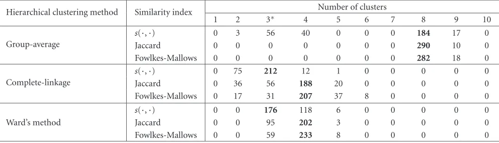
Table7: The estimated number of clusters for Leukemia dataset when measurements fromp=100 genes having the largest variance across tumor samples are used. The hypothesized number of clusters varies between 1 and 10. We represent in bold the maximum value over a row.

Hierarchical clustering method Similarity index Number of clusters

1 2 3∗ ₄ ₅ ₆ ₇ ₈ ₉ ₁₀

Group-average

s(·,·) 0 3 56 40 0 0 0 184 17 0

Jaccard 0 0 0 0 0 0 0 290 10 0

Fowlkes-Mallows 0 0 0 0 0 0 0 282 18 0

Complete-linkage

s(·,·) 0 75 212 12 1 0 0 0 0 0

Jaccard 0 36 56 188 20 0 0 0 0 0

Fowlkes-Mallows 0 17 31 207 37 8 0 0 0 0

Ward’s method

s(·,·) 0 0 176 118 6 0 0 0 0 0

Jaccard 0 0 95 202 3 0 0 0 0 0

Fowlkes-Mallows 0 0 59 233 8 0 0 0 0 0

calculating the value of the selected similarity indexsm. Re-peating the procedureNt=30000 times, we obtain for every similarity indexsmand for every allowed value ofk, a large set᏿k{smk,1,smk,2,. . .,smk,Nt}.

The histogram drawn for eachkfrom the correspond-ing set ᏿k plays the key role in the automatic estimation method introduced at the beginning of Section 5. To im-prove the accuracy, we base the estimation on several his-tograms for every k. This is performed by splitting each set ᏿k into Nb = 300 non-overlapping blocks and draw-ing a diﬀerent histogram for every block. Observe that the length of a block is N = 100. More precisely, we can write ᏿k=Ꮾk,1

Ꮾk,2

· · ·Ꮾk,Nb, where Ꮾk,i = {smk,(i−1)×N+1,. . .,smk,i×N}for 1 ≤ i ≤ Nb. Applying the newly introduced method, we estimate the number of clus-ters, which is assumed to lie between 1 andkmax, using only the blocksᏮ2,1,Ꮾ3,1,. . .,Ꮾkmax,1. This is done by computing

mk =median(Ꮾk,1) for 2≤k≤kmaxand then applying (7) and (8). Similarly, we obtain another estimation from the blocksᏮ2,2,Ꮾ3,2,. . .,Ꮾkmax,2. Continuing the procedure,Nb estimations of the number of clusters are resulting for ev-ery pair (clustering method, similarity index). For the case

kmax =10, we show inTable 7the distributions of estimated number of clusters when various similarity indices and HC algorithms are applied. For each distribution, we decide that

ˆ

Kis the value corresponding to the maximum number of oc-currences (represented in bold).

According to the existing biological knowledge, the num-ber of clusters for Leukemia dataset is three. Following the procedure described above, we obtain fromTable 7that ˆK= 3 only when complete-linkage, respectively, Ward’s method are used in conjunction with the new similarity indexs(·,·). Recall that for the simulated data, only complete-linkage and Ward’s method have produced good results. For Leukemia dataset, when these two HC algorithms are applied in combi-nation with Jaccard or Fowlkes-Mallows index, the estimated number of clusters is ˆK=4. A possible explanation for ˆK=4 relies on the remark, from [7], that ALL B-lineage type sam-ples can be further split into two clusters. Surprisingly, the group-average is leading to ˆK=8, which is hard to be given

a plausible biological interpretation. The experiments with Leukemia dataset reconfirm that the estimated number of clusters ˆK depends strongly on the HC algorithm and on the similarity index. The newly introduced indexs(·,·) is the only one that leads to correct estimations.

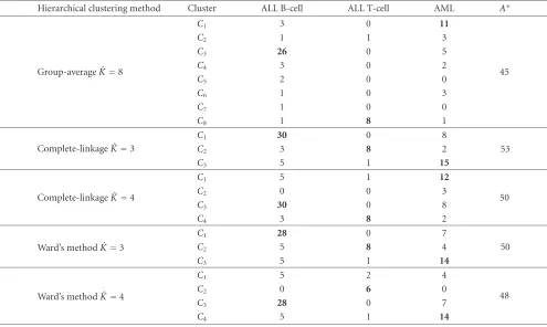
We further investigate how various HC algorithms clus-ter the 72×100 Leukemia dataset in classes when Euclidian distance is used to measure the distance between objects. We show inTable 8the contingency tables when the true parti-tion is compared with partiparti-tions produced by clustering algo-rithms for ˆK∈ {3, 4, 8}. In each case, we measure the degree of agreement between the compared partitions by computing the optimal assignment (A∗) as defined inSection 3.1: the larger the value of A∗, the better the degree of agreement. Remark that only the entries of the contingency matrix as-sociated with the optimal assignment (bold represented in

Table 8) correspond to samples reliably clustered. The values ofA∗ reported inTable 8vary between 45 (group-average) and 53 (complete-linkage), or equivalently, the proportion of reliably clustered samples varies between 63% and 74%.

As expected,A∗declines when the estimated number of clusters ˆK is larger than three. For ˆK = 3, the complete-linkage method clusters properly 30 samples from ALL B-cell class, 8 samples from ALL T-B-cell class, and 15 samples from AML class. When ˆK raises from 3 to 4, only the num-ber of samples from AML class, well classified by complete-linkage method, changes; namely, it decreases from 15 to 12. For ˆK ∈ {3, 4}, the number of ALL B-cell samples correctly grouped by Ward’s method is 28, and 14 AML samples are also well classified. In the case of Ward’s method, the num-ber of correctly grouped ALL T-cell samples drops from 8 to 6 when ˆKincreases from 3 to 4. It is obvious that the smallest

A∗is obtained for group-average for which ˆK=8; remark in this case that 8 ALL T-cell samples are assigned to the same group.

(13)

Table8: The contingency tables for the Leukemia dataset: the true partition given by a priori knowledge on the type of disease for each patient is compared with partitions produced by HC algorithms when ˆK∈ {3, 4, 8}. Only 100 genes having the largest variance across tumor samples are used for clustering. For each contingency table, the entries associated to the optimal assignment are represented in bold.

Hierarchical clustering method Cluster ALL B-cell ALL T-cell AML A∗

Group-average ˆK=8

C1 3 0 11

45

C2 1 1 3

C3 26 0 5

C4 3 0 2

C5 2 0 0

C6 1 0 3

C7 1 0 0

C8 1 8 1

Complete-linkage ˆK=3

C1 30 0 8

C2 3 8 2 53

C3 5 1 15

Complete-linkage ˆK=4

C1 5 1 12

50

C2 0 0 3

C3 30 0 8

C4 3 8 2

Ward’s method ˆK=3

C1 28 0 7

C2 5 8 4 50

C3 5 1 14

Ward’s method ˆK=4

C1 5 2 4

48

C2 0 6 0

C3 28 0 7

C4 5 1 14

[30], and also a special form, namely, leading principal com-ponents selection is investigated in [6]. In this paper, we fo-cus on the choice of the HC algorithm, respectively, the simi-larity index, and we refer for the feature selection problem to the rich literature on this topic.

6. CONCLUSION

In this study, we present a stability-based method applied for the estimation of the number of clusters in microarray data. To gain insights into the choice of the similarity index and HC algorithm, a careful study on simulated and real data is performed.

A new similarity indexs(·,·) is introduced, and its ca-pabilities are evaluated against other well-known similarity indices, based on a benchmark originally proposed in [21]. In this framework,s(P,P) takes small values when partition

P is obtained from partitionP after severemodifications, which recommends the use ofs(·,·) in practical applications. The indexs(·,·) is further evaluated in standard experimen-tal conditions when measuring the agreement between the true partition and the partition obtained at each level of an HC solution. We draw the conclusion that a value of 0.8 for

s(·,·) is likely to reflect the recovery of some part of the true structure. Moreover, since microarray data are noisy, when necessary to obtain grouping inkclusters, we do not choose

automatically the clusters at kth depth in the dendrogram, but move down the hierarchical tree until k nonsingleton clusters are identified.

We note the superiority ofs(·,·) and Jaccard when com-pared to Fowlkes-Mallows index. In experiments with sim-ulated data, the use ofs(·,·) was leading to the highest per-centage of recovering the true number of clusters five times, while Jaccard index three times and Fowlkes-Mallows index only once. Also for the Leukemia dataset,s(·,·) is the only index which leads to the correct estimation of the number of clusters ( ˆK =3). We emphasize that the definition ofs(·,·) relies on optimal assignment, which is the core of a visualiza-tion tool newly proposed in this paper for the interpretavisualiza-tion of microarray data clustering.

The good performances of complete-linkage algorithm and Ward’s method, observed in Section 5.1 for artificial data, have been reconfirmed for Leukemia data. Even when basing the clustering only on 100 selected genes, the results in

(14)

complete-linkage or Ward’s method are well suited to be used with the newly introduced method for the estimation of the number of clusters. The resulting method will offer reliable estimates forKand at the same time will be very fast since the HC is computationally efficient; the same tree can be used for all values ofk∈ {2, 3,. . .,kmax}by looking at different levels of the tree each time. OnceKis estimated, partition meth-ods can be further employed for assigning the objects to the clusters.

APPENDICES

A. PROOFS OF PROPOSITIONS

Proof ofProposition 1. It results from the definition that

D(P,P)= D(P,P)≥ 0 for each pair of partitions (P,P), while D(P,P) = 0 if and only if PandPare identical. It remains to verify the triangle inequality. Consider three par-titionsP,PandPof the objects inT. LetU(andV) de-note the minimal subset ofT which must be removed such that the induced partitions on P andP (resp., onP and

P) are identical. RemovingUVfromTinduces identical partitions onP,P, andP, which leads to the chain of in-equalities and in-equalities:D(P,P)≤ |UV| ≤ |U|+|V| =

D(P,P) +D(P,P).

Proof ofProposition 2. Since all entries ofMare nonnegative integers and their sum isN >0, there exist at least one entry

mi j such thatmi j > 0. This leads toA(P,P)≥ 1 which is equivalent toD(P,P)≤N−1. WhenP = {P1,P2,. . .,PN} with |P1| = |P2| = · · · = |PN| = 1 andP = {T}, the matrixMreduces to a column vector having only ones as en-tries, which implies thatD(P,P)=N−1. Conversely, when

D(P,P)=N−1 and|P| =r ≥c= |P|, letmi j=1 be the only entry ofMwhich is considered in the computation of the optimal assignmentA(P,P)=N−D(P,P)=1. Since no entry of the columns with indexes diﬀerent of jis con-sidered in A(P,P), it follows that all the columns contain only zeros, so,Mis essentially a column vector. Because this column vector does not have any entry larger than one, the partition Pconsists of a single cluster and the partition P

consists only of clusters containing single-objects.

B. A LOWER BOUND FORE[s(·,·)]UNDER THE HYPOTHESIS OF GENERALIZED HYPERGEOMETRIC DISTRIBUTION

Proposition B.1. Under the assumption of fixed marginsmi·

andm·j, and random allocation of matching counts tomi j,

Es(P,P)≥ 1

N−1 c

i=1α(i)β(i)

N −1

≥ 1

N−1 c i=1α(i)

c −1

,

(B.1)

whereα(1),α(2),. . .,α(r)andβ(1),β(2),. . .,β(c)are the elements

of the set{α1,α2,. . .,αr}, respectively, the set {β1,β2,. . .,βc}

decreasingly ordered.

Proof. Consider the particular assignment valuea(P,P)

c

i=1m(i),(i). By definition, A(P,P) ≥ a(P,P), and con-sequently, E[A(P,P)] ≥ E[a(P,P)]. This observation, to-gether with definition (3) andE[a(P,P)]=c

i=1α(i)β(i)/N, proves the first inequality in (B.1). The second inequality re-sults from the Chebyshev inequality [31] applied for the se-quences (α(1),α(2),. . .,α(c)) and (β(1),β(2),. . .,β(c)); we also used the identityci=1β(i) = N. Note that the equality oc-curs if and only ifα(1) =α(2) = · · · =α(c)orβ(1)=β(2) = · · · =β(c).

Corollary B.1. (a) Whenr > c, the maximum value of the lower bound,

max α1,α2,...,αr

1

N−1 c i=1α(i)

c −1

=1

c N−r

N−1, (B.2)

is achieved wheneverα(c+1)=α(c+2)= · · · =α(r)=1. (b)Whenr=c, the expression of the lower bound becomes

(1/(N−1))(N/c−1).

C. ASYMPTOTIC AND FINITE SAMPLE

CHARACTERISTICS FOR THE SIMILARITY INDICES

We illustrate the computation of s(P,P) by considering an example from [21]: two partitions of six objects, P = {{x1,x2,x3},{x4,x5,x6}} and P = {{x1,x2},{x3,x4,x5}, {x6}}. Elementary calculations lead tos(P,P)=0.6 which is equal to the Rand index value reported in [21]. The same ex-ample was used in [25] to compare RandHA, which takes the value 2/17≈0.1176, with RandMA=1/3≈0.3333. For this particular case, s(·,·) and Rand index take the same value which is larger than the adjusted forms of Rand. We consider in this section more comparisons of the newly introduced index with Rand, RandHA, RandMA, Jaccard, and Fowlkes-Mallows indices.

To study the finite and asymptotic characteristics, assume that the original data partitionPconsists ofKclusters withn

objects each; ten cases whenPis obtained fromPafter vari-ous simple and major modifications are considered. This ap-proach was firstly proposed in [21] to establish some formal properties of Rand index and further used in [9] when eval-uating the performances of the Fowlkes-Mallows index. The expressions of Rand, RandMA, Jaccard, and Fowlkes-Mallows indices for all the ten cases are given in [23]. We compute in Table C.1the close forms for the partition distance and the indexs(P,P) whenPis obtained by modifyingPas de-scribed in [21].

We compute also the asymptotics when the number of objects in each cluster increases without bound (n → ∞), while the number of clusters is fixed (K fixed). We observe from the fourth column inTable C.1that the index asymp-totics for the fourth and fifth scenarios are equal to 1.0, which is also true for all similarity indices analyzed in [23]. As it was already pointed out in [23], this is reasonable since

(15)

TableC.1: Expressions for the partition distanceD(·,·) and the indexs(·,·) between two similar partitions, given an initial partitionP which hasKclusters ofnobjects each.

Pis a simple modification of the original partitionP

Modification ofP D(P,P₎ _s₍_P_,_P₎ limn→∞s(P,P) limn→∞s(P,P)

Kfixed K=λn

Two clusters joined n n(K−1)−1

nK−1

K−1

K 1.0

One cluster splits into

two equal parts (neven) n/2

n(K−1/2)−1 nK−1

K−1/2

K 1.0

One cluster splits into

single-object clusters n−1

n(K−1) nK−1

K−1

K 1.0

One object taken from each cluster

to form a new cluster ofKobjects K

(n−1)K−1

nK−1 1.0 1.0

PandPare similar modifications of the original partitionP

Diﬀerences betweenP_and_P _D₍_P_,_P₎ _s₍_P_,_P₎ limn→∞s(P,P) limn→∞s(P,P)

Kfixed K=λn

Movement of an object

to diﬀerent clusters 1

nK−2

nK−1 1.0 1.0

Diﬀerent clusters split into two

equal parts (neven) n

n(K−1)−1 nK−1

K−1

K 1.0

Diﬀerent pairs of clusters

joined 2n

n(K−2)−1 nK−1

K−2

K 1.0

Pis a major modification of the original partitionP

Modification ofP D(P,P₎ _s₍_P_,_P₎ limn→∞s(P,P) limn→∞s(P,P)

Kfixed K=λn

All clusters joined into

one large cluster n(K−1)

n−1

nK−1 1/K 0.0

All clusters split into

single-object clusters (n−1)K

K−1

nK−1 0.0 0.0

nclusters are formed withK objects in each, one object from each original cluster

nK−min(n,K) min(n,K)−1

nK−1 0.0 0.0

The asymptotic values fors(P,P) and the Jaccard index co-incide for seven out of ten evaluated situations, while the asymptotics of Jaccard index never exceed the asymptotics of Fowlkes-Mallows index [23]. Comparing the expressions of Jaccard and Fowlkes-Mallows indices given inSection 3.1, it is easy to prove that the Jaccard index cannot be larger than the Fowlkes-Mallows index when both are well defined. We pay particular attention to the behavior of the similarity in-dices for the last three scenarios (severe cases). The asymp-totics fors(P,P) are 0.0 in the last two cases (identical with the values of RandMAand Jaccard), which shows the supe-riority ofs(·,·) when comparing with the Rand index. The value reported for Rand in [21] in both cases is (K−1)/K, and seems unacceptable since it is too close to 1.0. For the nineth modification, the Fowlkes-Mallows index is not de-fined, while for the tenth modification, it is equal to 0.0. The asymptotic value ofs(P,P) is 1/K when the modifica-tion is such that all clusters are joined into one large cluster,

and being smaller than 0.5 for anyK ≥ 2, it may be con-sidered acceptable. For that case, Rand and Jaccard are also equal to 1/K, while Fowlkes-Mallows is larger (1/√K) and RandMA=0.0.

WhenKis allowed to increase without bound (K→ ∞),

nmust also increase without limit, and the solution is to let

Kincrease as a simple proportion ofn(K=λn) [9]. The re-sults are reported in the last column ofTable C.1: only in the severe cases, the computed value is 0.0, while for other situ-ations is 1.0. The behavior is identical for RandMA, Jaccard, and Fowlkes-Mallows indices, while Rand is equal to 1.0 for the last two severe cases.

Considering an example based on fixed values fornand

K,Table C.2compares diﬀerent indices whenn = K = 4. The severity of the modification from the true clustering is ranked as in [23], where Rand, RandMA, Fowlkes-Mallows and Jaccard similarity measures have been compared forn=