Earth Planets Space,54, 1219–1236, 2002
Acquisition, processing and analysis of densely sampled P- and S-wave
OBS-data on the mid-Norwegian Margin, NE Atlantic
Rolf Mjelde1∗, Tommy Timenes2, Hideki Shimamura3, Toshihiko Kanazawa4, Hajime Shiobara3∗,
Shuichi Kodaira3∗∗, and Ayako Nakanishi3∗∗
1Institute of Solid Earth Physics, All´egt. 41, University of Bergen, 5007 Bergen, Norway 2Institute of Solid Earth Physics, University of Bergen, 5007, Norway 3Institute for Seismology and Volcanology, Hokkaido University, Sapporo 060, Japan
4Earthquake Research Institute, University of Tokyo, Tokyo 113-0032, Japan
(Received April 11, 2002; Revised November 2, 2002; Accepted November 8, 2002)
This paper describes the processing and analysis of semi-local OBS-data shot along a 122 km profile in the Vøring Basin, NE Atlantic margin, using both a high-frequency/short spacing and a low-frequency/long shot-spacing air-gun source. Spectral analysis of the data reveals that an important difference between the two sources used, is that the low-frequency source generates significantly more energy around 6 Hz. This higher content of very low frequencies allows detection of arrivals to larger offsets for the low-frequency source. For the nearest offsets (0–20 km) the high-frequency source is able to resolve some more details than the low-frequency source, as far as the shallow to intermediate sedimentary levels are concerned. This is mainly caused by the fact that the high-frequency source has a much sharper primary pulse and reduced bubble pulse compared to the low-frequency source. The data quality can be significantly enhanced by use of band-pass filtering, trace mixing, FK (velocity) filtering, minimum phase predictive deconvolution, as well as Radon filtering. Inspection of particle diagrams documents S-wave splitting, interpreted as microcracks aligned vertically in the sedimentary section by the present day (slightly compressive) stress-field.
1.
Introduction
On the Norwegian continental shelf, NE Atlantic, several regional crustal scale seismic experiments by use of Ocean Bottom Seismographs (OBS) have been performed in col-laboration between University of Bergen and Hokkaido Uni-versity. An extensive experiment involving Japanese OBSs was performed in 1988 off Lofoten, northern Norway (Fig. 1, Sellevollet al., 1988). The analysis of these data has shown that this method in many cases provides information about the crustal structure not achievable through the study of seis-mic multichannel vertical-incidence data alone (Mjelde et al., 1992, 1993). Of particular importance is the ability of the OBS technique to reveal structures beneath a flood-basalt, which in this area is opaque using the multichannel reflection method. In addition, the horizontal components ensure reliable analysis of S-waves, which provides infor-mation about lithology, as well as anisotropy caused by frac-tures and aligned minerals (Mjeldeet al., 1995).
In spite of the well documented efficiency of the method, only minor efforts have been made to investigate how the method can assist in more detailed investigations of
sedimen-∗Present address: Earthquake Research Institute, University of Tokyo,
Yayoi 1-1-1, Bunkyo-ku, Tokyo 113-0032, Japan.
∗∗Present address: JAMSTEC, 2-15 Natsushima-cho, Yokosuka-city,
Kanagawa 237-0061, Japan.
Copy right cThe Society of Geomagnetism and Earth, Planetary and Space Sciences (SGEPSS); The Seismological Society of Japan; The Volcanological Society of Japan; The Geodetic Society of Japan; The Japanese Society for Planetary Sciences.
tary basins and crystalline crustal structure. Deep structures (crystalline basement and the Moho) can be mapped with confidence from OBS data, but detailed imaging of structures is generally impossible due to the long distance between the OBSs (20–30 km) and shots (ca. 250 m) used in regional sci-entific crustal studies. In addition, the seismic source gener-ally used in such experiments is focused on low-frequencies (5–20 Hz), and its pulse is often contaminated by large bub-bles.
To enlighten these aspects and to evaluate the resolution limits of OBSs used in mapping of crustal structures, an ex-tensive experiment by use of twenty-five three-component OBSs deployed along a 122 km long profile was conducted in the central Vøring basin in 1992 (Fig. 1). This basin was influenced by intense magmatism during the early Tertiary opening between Greenland and Norway (e.g. Eldholm and Grue, 1994), making mapping of deep sedimentary and crys-talline structures very difficult with multichannel reflection data.
The profile was acquired twice; first with a low-frequency source shot every ca. 250 m. In the regional study only five of the twenty-five OBSs were used (OBS 1, 6, 13, 17, 20), whereas all OBSs were included in the semi-local (low-frequency source) study. The profile was then shot with a frequency source fired every ca. 50 m (semi-local, high-frequency study). The modeling of the regional and semi-local data shot with the low-frequency source (both P- and S-waves), has been presented by Mjeldeet al. (1997a, b) and
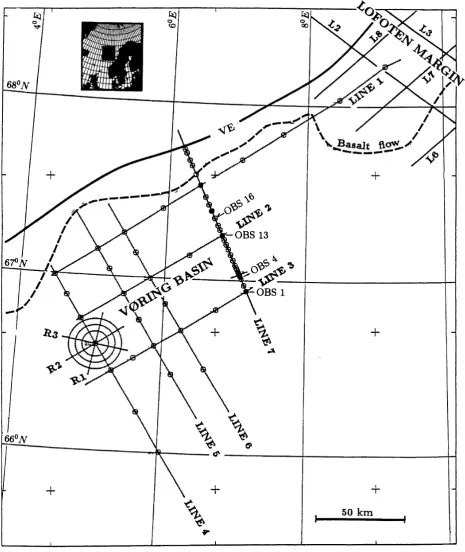
Fig. 1. The survey area with all profiles and OBS positions indicated. Line 7 represents the semi-local profile described in this paper. The landward limit of the early Eocene basalt flow, the Vøring Escarpment (VE), and parts of the profiles acquired off Lofoten in 1988 are also indicated.
Digranes et al. (1996). The main purpose of the regional study was to map the distribution of sills in the sediments, the deep sedimentary structures, the top of the crystalline base-ment, the distribution of an inferred lower crustal magmatic body, and the depth to the Moho. The purpose of the (low-frequency source) semi-local study was to evaluate the accu-racy of the regional method, and to evaluate the importance of closer OBSs spacing in a more detailed mapping of struc-tures throughout the crust. The main reason for including
the S-waves in the analysis was these waves’ general abil-ity to provide lithological information when combined with P-waves (e.g. Neidell, 1985).
R. MJELDEet al.: ANALYSIS OF DENSELY SAMPLED OBS-DATA ON THE MID-NORWEGIAN MARGIN 1221
Fig. 2. Theoretical amplitude spectrum of far-field signature for the high-frequency source (blue) and low-frequency source (red). In order to allow comparison of the relative differences in amplitude versus frequency, the spectra have been adjusted for differences in total output power.
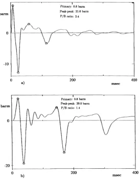
Fig. 3. Theoretical seismic pulse (far-field signature) for the high-frequency source in (a) and low-frequency source in (b).
enhanced resolution and possibilites for more sophisticated processing.
2.
Data Acquisition
The location of OBSs and profiles shot during the experi-ment in the Vøring basin in 1992 are shown in Fig. 1. Each of the OBSs was deployed several times; a total of 75 OBS
sec-ond time (Berget al., 2001), a circle-shooting around one of the OBSs deployed in the regional survey, and a semi-local experiment where 25 OBSs were employed a third time. This paper focuses on the data acquired during the semi-local sur-vey.
Two different air-gun configurations were used during the experiment. Four equally sized Bolt 1500 C air-guns with a total volume of 4800 in3(78.7 l), were used in all parts of the
acquisition (Figs. 2–3). This high-energy source with main frequency spectrum in the range 5–40 Hz, was used to allow mapping of deep structures. The second configuration con-sisted of two Bolt 1500 C air-guns with waveshape together with five air-guns on a string with a total volume of 1956 in3 (32.1l) (Figs. 2–3). The size of these air-guns varied from 60 to 340 in3. This air-gun configuration with main frequency spectrum in the range 8–42 Hz, was used during the local and semi-local study, because of its increased content of higher frequencies and better pulse/bubble ratio. This source con-figuration was thus used to allow better mapping of shallow and intermediate crustal structures. One shot was fired ev-ery 2 min. at about 250 m intervals when the low-frequency source was used, and every 1 min. at about 50 m intervals for the high-frequency source. The source depth was 12 m in each case. The distance between each gun was ca. 4 m, which implies linear interaction between the air-guns, and the extent of each air-gun array was limited, implying that both sources can be considered as point-sources.
The three-component OBSs used were developed at the Institute for Seismology and Volcanology, Hokkaido Uni-versity, and Laboratory for Earthquake Chemistry, Tokyo University. These analogue instruments equiped with 4.5 Hz geophones could record continuously for 14 days within the 1–30 Hz frequency range (−3 dB). Two different tape-speeds were used during the experiment; a low tape-speed for the regional study, limiting this survey to frequencies be-low about 20 Hz, and a high tape-speed for the semi-local and local studies, allowing detection of frequencies up to ca. 40 Hz. The reader is referred to Kanazawa (1993) and Mjeldeet al.(1997a) for more details concerning the instru-ments used.
The OBSs recorded continuously throughout the acquisi-tion of the semi-local dataset. The posiacquisi-tions and thus the state of coupling between the instruments and the seafloor were the same during the shooting with both sources. The shot-direction was also the same (from NW to SE), assuring that differences in the two datasets can be related to three aspects only; the ambient noise level, the sources, and the shot-distance (in average 233 m for the low-frequency data, and 55 m for the high-frequency data).
3.
Regional versus Semi-Local Models
The regional kinematic P-wave model derived by ray-tracing of 5 OBS vertical components, acquired by use of the low-frequency source, is shown in Fig. 4(a) (Mjeldeet al., 1997a). The ray-tracing software employed has been devel-oped by Norsk Hydro (Pajchelet al., 1989). The basins and highs down to the ‘lowest reflector’ (lr) have been accurately mapped by a multichannel reflection profile acquired earlier, whereas the deeper layers have been included based on the OBS-data. The high-velocity sill-intrusions in the
sedimen-tary section, indicated as thin, darker shaded layers in the model, also result from the modeling of the OBS-data. These sill-intrusions are assumed to be emplaced during the early Eocene break-up between the European and north American plates. The high-velocity lower crust, which is inferred to represent intrusions in the lower crust (magmatic underplat-ing), are also included in the model based on the OBS-data.
The semi-local P-wave model derived by ray-tracing of all 25 OBS vertical components acquired along the same profile (with the same source) is shown in Fig. 4(b) (Mjeldeet al., 1997b). Two observations are clear by comparing the re-gional and semi-local models; firstly, the over-all structures are very similar, proving that the regional method provides reliable regional models, and secondly, that the semi-local data provide more detailed information in all parts of the model. Whether these ‘details’ are important enough to sug-gest use of the more time-consuming and expensive semi-local experiment set-up, would depend on the scientific ob-jectives in each specific case.
4.
Data Recovery
All twenty-five OBSs used in the semi-local study dis-cussed in this paper were recovered from the sea-floor, but the tape from OBS 2 was blank due to malfunctioning of the tape recorder. This applies, of course, to the shooting with both sources. In addition, a few traces for each OBS could not be recovered. The reasons for the loss of these traces can be related to problems with the seismic source, as well as minor anomalies in the A/D conversion procedure. For the shooting with the low-frequency source 2–3 traces were lost for each OBS, with the exception of OBS 13 and 17, for which 27 and 93 traces were lost, respectively. This im-plies a total loss of 5.3% for the low-frequency data. For the high-frequency data, the variations in the loss of data were higher; most of the OBSs lack 2–4 traces only, but the data from OBS 17 could not be A/D converted due to strong noise of unknown origin. For the remaining OBSs, the largest loss of data is found on OBS 9 (63 traces). The total data-loss for the high-frequency data is 8.5%. It is important to under-line that this limited loss of data (for both sources) does not significantly hamper the attempts to evaluate the differences between the acquisitions, nor does it significantly reduce the amount of geological information that can be extracted from the datasets.
5.
Data Processing
The OBS-data were A/D converted at Hokkaido Univer-sity in Sapporo, and further processing were performed at the Institute of Solid Earth Physics (IFJ), University of Bergen. The digital data-processing of the low-frequency vertical components was limited to frequency filtering only, as far as the semi-local P-wave modeling was concerned (Mjelde
et al., 1997b). For the horizontal components, spiking de-convolution was applied in addition, in order to assure more accurate detection of S-wave first breaks (Digranes et al., 1996).
struc-R. MJELDEet al.: ANALYSIS OF DENSELY SAMPLED OBS-DATA ON THE MID-NORWEGIAN MARGIN 1223
Fig. 4. (a) The regional model for profile 7, with seismic P-wave velocities (in km/s) for some main layers indicated (from Mjeldeet al., 1997a). ‘lr’ refers to the deepest interface mapped from multichannel reflection data, and ‘cb’ is interpreted as the top of the crystalline basement. (b) The semi-local model derived from the data acquired with the low-frequency source. The velocities are very similar to those in (a) (from Mjeldeet al., 1997b).
tures along the profile. To limit the number of figures in the paper, and since the processing of the four OBSs did not re-veal significant differences, we will focus on the processing of OBS 1. Unless otherwise stated, the processing schemes described have been applied to the vertical-, as well as to both horizontal components. The processing has been per-formed by use of the PROMAX software. Detailed back-ground for each processing step is not given, since only stan-dard routines for processing of surface seismic data have been applied.
5.1 Analysis of frequencies, amplitudes and noise
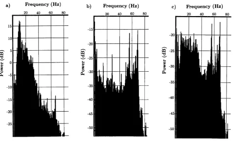
Fig. 5. Examples of typical amplitude spectra for OBS 1, shot with the high-frequency source. (a) Signal spectrum for traces 1989–2016, non-reduced time-window 3.1–5.1 s. (b) Low- and high-frequency noise spectrum for traces 298–307, non-reduced time-window 5–8 s. (c) Seismic frequency noise spectrum for traces 348–357, non-reduced time-window 2–5 s. As dB is relative unit, only relative comparisons between the vertical axis of the three plots can be made.
et al., 1989). In addition to this low-frequency noise, sev-eral peaks are observed in the 50–70 Hz frequency-range (Fig. 5(b)). These frequencies are recorded with large distor-tions, since the analogue tape recorder with the tape-speed used cannot record frequencies above 40 Hz correctly. The high-frequency peaks are most likely instrumental noise.
The low- and high-frequency noise do not represent any problems for the analysis of the data, since these frequency bands can be effectively removed using a band-pass filter. For many traces, however, large amplitude noise is present throughout the seismic frequency-window (ca. 5–35 Hz). Note the much higher level of noise for this band if fre-quencies in Fig. 5(c), compared with Fig. 5(b). This noise is either caused by a nearby seismic vessel (no such vessels were reported to be present in the area) or a vessel of an-other type (cargo/fishery). Moreover, it cannot be excluded that parts of the noise might represent water-arrivals from our own previous shots, although the magnitude and spa-tial distribution of the noise precludes this component to be large. The noise appears as strongly dipping coherent events that are best observed in the high-frequency data, due to the closer shot-spacing for these data (Fig. 8(a)). We will in the following refer to this noise as seismic, since it is constrained within our usable seismic bandwidth. This seismic noise do not represent any severe problem as far as the quality of the OBS-data is concerned, since it can be attenuated by pro-cessing, and since its dip differs significantly from that of the real seismic arrivals recorded on the OBSs.
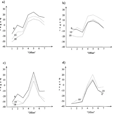
The seismic noise induces a problem, however, when the decay of the amplitudes for different signal-frequencies are
investigated, following the procedure described by Mjelde
et al. (1997c). Figures 7(a) and (b) shows the power of the three dominant signal frequency-peaks, 6, 10 and 18 Hz, as function of offset. The power has been calculated in a 2 s window covering the first arrivals, as well as lower amplitude secondary arrivals. In Figs. 7(c), (d) the plots have been corrected for seismic noise. This correction is performed as follows; for traces with no apparent seismic noise, the power in the 3–40 Hz range is observed to be about −37 dB (ambient noise-level). For traces where the seismic noise is observed, it is assumed that the level of the ambient noise remains constant across the signal time-window. The level of the seismic noise is then measured for the three investigated frequency-peaks (from the noise spectra), and subsequently subtracted from the signal power-spectrum. It is important to notice that the correction is not performed for the near-zero offsets, since the short travel-time of the direct wave prevents accurate estimates of the noise-level for these traces.
R. MJELDEet al.: ANALYSIS OF DENSELY SAMPLED OBS-DATA ON THE MID-NORWEGIAN MARGIN 1225
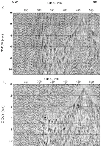
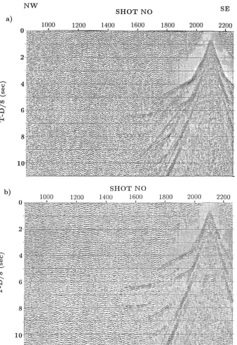
Fig. 6. (a) Vertical high-gain component of OBS 1, low-frequency data. Plotted with Automatic Gain Control (AGC) window of 4 s length, and 8.0 km/s reduction velocity. (b) Same as (a), but 5–12 Hz band-pass filtered in addition. Notice that the far-offset arrival between shotpoints 290 and 340 appears much more clearly after filtering. The arrow at ca. 450 indicates an arrival that is more clearly defined in the data acquired with the high-frequency source (compare with Fig. 8(b)), whereas the far-offset arrival at ca. 320 is clearly observable only in the low-frequency data.
which allows detection of arrivals to larger offsets. This can be seen by comparing the high-frequency data shown in Fig. 8 with the low-frequency data presented in Fig. 6; the low-frequency data reveal a strong arrival at ca. 6.5 s depth, between shotpoints 290 and 340, which cannot be seen in the high-frequency data.
5.2 Differences between sources and shot-spacing
The difference in low-frequency content between the two sources implies that coherent seismic energy can be observed to larger offset on the data acquired with the low-frequency source. Although the shot-spacing is about 4 times larger for the low-frequency data, arrivals can generally be observed to
larger offset in these data; to 59 km (mean maximum offset for all OBSs), compared to 53 km for the high-frequency data. The maximum offset for a single OBS is 88 km for the low-frequency data and 63 km for the high-frequency data. (All twenty-five OBSs have been included in this analysis.)
Fig. 7. Power spectra for the three frequency peaks studied for OBS 1; 6, 10 and 18 Hz. (a) and (b) show the uncorrected estimates for the low- and high-frequency source, respectively. (c) and (d) show the corresponding corrected curves (see text). ‘Offset’ refers to a representative selection of arrivals for various offset that have been studied; arrival 1 being the fartest offset arrival to the NW, arrival 5 represents the near offsets, and arrival 7 represents offsets close to the SE end of the profile. Detailed offset ranges (shot no) for the low-frequency data, arrivals 1–7: 298–307, 348–357, 379–388, 429–438, 456–465, 487–496, 513–522. Detailed offset ranges (shot no) for the high-frequency data, arrivals 1–7: 1359–1395, 1609–1645, 1766–1802, 1989–2016, 2070–2110, 2150–2183, 2210–2242.
mainly caused by the fact that the high-frequency source has a much sharper primary pulse and reduced bubble pulse com-pared to the low-frequency source. In addition, a slightly in-creased level of higher frequencies (above 15 Hz; Fig. 7) also contributes to the differences in resolution.
Plotting every 4th trace of the high-frequency data gen-erally causes a decrease in the maximum offset of clearly identifiable arrivals, compared to the complete seismic sec-tion. Decreasing the spacing between the shots thus clearly increases the useful penetration depth of the survey (Fig. 8). However, the higher content of frequencies around 6 Hz in the low-frequency data assures larger penetration depth for that survey, in spite of the coarser shot interval applied.
5.3 Trace mixing
Trace mixing is a method that can be used to enhance the coherency of weak far-offset arrivals, and hence decrease the uncertainty in the interpretation of these arrivals (e.g. Samson et al., 1995). When applied to data reduced by 8 km/s, trace mixing will enhance arrivals that propagate with an apparent velocity of about 8 km/s (horizontally) and reduce the amplitudes of dipping arrivals.
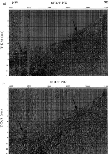
The trace mixing consisted of multiplying the trace sam-ples by the following weights: 1, 2, 1 for the low-frequency data, and 1, 2, 3, 4, 5, 4, 3, 2, 1 for the high-frequency data. The accumulated weighted sample is subsequently normal-ized by the sum of the weights. These number of traces have been used in order to sum traces for comparable offsets. Fig-ure 9(b) shows an example of the result of weigthed trace mixing, where 3 traces have been applied in the mixing for the high-frequency data (every 4th trace plotted). Compar-ing with the plot with no trace mixCompar-ing applied (Fig. 9(a)), it is clear that low-velocity dipping events have been attenu-ated, and that the continuity of the far-offset arrivals has been increased. Furthermore, the far-offset arrival seen between shotpoints 290 and 340 in the low-frequency data (Fig. 6(b)), but not observed in the high-frequency data for the same off-sets (between shotpoints 1350 and 1550; Fig. 9(a)), can be weakly distinguished after trace mixing.
R. MJELDEet al.: ANALYSIS OF DENSELY SAMPLED OBS-DATA ON THE MID-NORWEGIAN MARGIN 1227
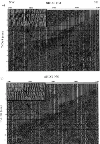
Fig. 8. (a) Vertical high-gain component of OBS 1, high-frequency data. Plotted with 4 s AGC, 8.0 km/s reduction velocity, and 5–12 Hz band-pass filter. The arrow at ca. 1450 indicates an arrival that is weakly observable (compare with Fig. 6(b)), and the arrow at ca. 1250 shows an axample of ‘seismic noise’. (b) Same as a), but every 4th trace plotted only. The arrow at ca. 2000 indicates an arrival that is more clearly defined than in the data acquired with the low-frequency source (compare with Fig. 6(b)). The arrow at ca. 1450 shows that the arrival weakly observable in (a), cannot be discerned when every 4th trace only is plotted.
induces similar coherency within the noise. In addition to the trace mixing described above, the mixing has also been applied along other dips, i.e. on data reduced with velocities below and above 8 km/s, without apparent enhancement of the data.
One limitation of the applied trace mixing is that it re-quires arrivals to be reasonably horizontal across the mixed traces. For our complicated dataset this requirement is only partly fulfilled. It must thus be expected that this kind of pro-cessing would be more successful when applied to data from geologically simpler areas.
5.4 FK (velocity) filtering
The high-frequency data are spatially aliased to a small degree only, consequently arrivals with velocity above about 1.5 km/s can be removed by filtering in the FK (frequency-wavenumber) domain. The long distance between the traces for the low-frequency data, however, causes spatial aliasing for velocities below about 5.5 km/s.
Fig. 9. (a) Vertical high-gain component of OBS 1, high-frequency data. Every 4th trace plotted with 4 s AGC, 8.0 km/s reduction velocity, and 5–12 Hz band-pass filter. (b) Same as (a), but with trace mixing (3 traces) in addition. Notice that the deep far-offset arrival clearly seen in Fig. 6(b) can be seen, although weakly, between trace no. 1350 and 1550.
5.5 Deconvolution
Figure 11(b) shows an example of high-frequency data after deconvolution, compared to the non-deconvolved data in Fig. 11(a). The deconvolution applied is minimum phase predictive deconvolution with 500 ms operator length and 32 ms prediction gap. The design window follows the first arrival, and its length is 4 s from about 100 ms before the first arrival.
The deconvolution applied clearly removes “ringing” from the data, and the onset of the different arrivals can be inter-preted with larger certainty. This is true for both datasets, although the effect is larger for the high-frequency data.
5.6 Radonfiltering
R. MJELDEet al.: ANALYSIS OF DENSELY SAMPLED OBS-DATA ON THE MID-NORWEGIAN MARGIN 1229
Fig. 10. (a) Horizontal high-gain component (channel 1) of OBS 1, high-frequency data. Plotted with 4 s AGC, 8.0 km/s reduction velocity, 5–14 Hz band-pass filter and trace mixing (3 traces). (b) Same as (a), but an FK filter removing apparent velocities below 2 km/s and above 5 km/s has been applied in addition. Notice the much clearer appearence of the intermediate velocity arrivals.
5.7 Multichannel processing
Conventional multichannel processing has been success-fully performed on the local dataset, which was acquired by use of the high-frequency source and twenty OBSs (Berg
et al., 2001; see Section 2). The shot- and receiver spac-ing were 50 and 200 m, respectively. The main differ-ences from standard multichannel processing resulted from the more complex geometry; the depth of the OBSs varied slightly, and the distance between the OBSs were not con-stant. The location of the OBSs on the seafloor were de-termined to within 20 m uncertainty by use of acoustic
tri-angulation (Shiobaraet al., 1997). The reader is refered to Berg et al.(2001) for details concerning the multichannel processing of the local dataset. The quality of the horizontal component stack allowed interpretation of S-wave reflectors on hydrocarbon reservoir scale to be made. These reflec-tors were better imaged on the vertical component (P-wave) stack (Fig. 15), but the quality of these processed data were not as high as that of the multichannel surface seismic data acquired earlier (Mjeldeet al., 1997a).
Fig. 11. (a) Horizontal high-gain component (channel 1) of OBS 1, high-frequency data. Plotted with 4 s AGC, 8.0 km/s reduction velocity, and 5–14 Hz band-pass filter. (b) Same as (a), but with predictive deconvolution in addition. Notice the reduction of ‘ringing’.
limited success due to the coarse OBS spacing. Although it cannot be excluded that more sophisticated multichannel processing of the semi-local data may provide more postive results, it is recommended that the receiver spacing is kept below ca. 2 km in multichannel studies.
6.
Hodogram Analysis
Complete use of three-component seismic data includes an analysis of particle diagrams, or hodograms. Such anal-ysis often reveals S-wave anisotropy, that could result from fluid-filled microcracks aligned vertically by the present day stress-field (e.g. Crampin, 1990). In such an anisotropic me-dia an incoming S-wave would split into two S-waves, one
polarized along the microcracks and one polarized perpen-dicular to the microcracks. The wave polarized along the microcracks will propagate with higher velocity, inducing a characteristic splitting of the waves that can be observed in hodograms.
In order to facilitate the analysis, the horizontal com-ponent high-frequency data have been rotated into in-line (along the shot profile) and cross-line (perpendicular to the profile) components, using the polarization of the direct (P-wave) water-arrival. The uncertainty in such rotations for this dataset have been estimated to±5% by Digraneset al.
(1996).
anal-R. MJELDEet al.: ANALYSIS OF DENSELY SAMPLED OBS-DATA ON THE MID-NORWEGIAN MARGIN 1231
Fig. 12. (a) Horizontal high-gain component (channel 1) of OBS 1, high-frequency data. Plotted with 4 s AGC, 8.0 km/s reduction velocity, and 5–14 Hz band-pass filter. (b) Same as (a), but after application of radon filtering. Notice the appearance of a deep high-velocity arrival, barely interpretable before filtering.
ysis of our data. Two intermediate depth PPS arrivals are indicated on the in-line component in Fig. 13(a). These ar-rivals propagate with apparent P-wave velocities, and rep-resent waves that have been P-to-S converted on the way up (Mjeldeet al., 2002). Figure 13(b) shows how the two arrivals, labelled A and B, are shifted in time between the in-line and cross-line components, suggesting that they rep-resent arrivals that have propagated with different velocities on the way up. This is confirmed by studying the hodograms (Fig. 14), which demonstrates that the two first arrivals are polarized at 10–30◦angle from the in-line direction, whereas the second arrivals are polarized at ca. 70◦ angle from the
first arrivals. This could be interpreted in terms of fluid-filled microcracks aligned vertically, striking 10–30◦SW of the az-imuth of the profile.
Fig. 13. (a) In-line horizontal high-gain component of OBS 1, high-frequency data. Plotted with 4 s AGC, 8.0 km/s reduction velocity, 5–14 Hz band-pass filter, and FK filter (arrivals with apparent velocities below 2 km/s removed). Arrivals A and B have been studied with hodograms. (b) Left: Blow-up of portion of (a). Right: Same blow-up (and processing) of the cross-line component. Note the delay of arrivals compared with the in-line plot.
In our case, a rough identification of phases can be done by comparisons with the modeling of the low-frequency data (Digraneset al., 1996). Comparisons between estimates of splitting and propagation depths indicates that the splitting increases with propagation depth, from ca. 200 ms for in-termediate sedimentary arrivals to a maximum of ca. 500 ms for crystaline crustal arrivals. This could be interpreted as vertical microcracks extending throughout the tary section. The average anisotropy in the entire sedimen-tary section would, based on these phase identifications, be in the order of 7%. These observations confirm the results of Digraneset al. (1996), who estimated NW-SE alignment of microcracks extending down to deep sedimentary levels, as well as in the lower crust, based on azimuthal anisotropy modelled from crossing profiles. These authors did not con-strain their results by use of particle diagrams. The amount of anisotropy was estimated by Digraneset al. (1996) to be 5%. The direction of fast direction corresponds to other mea-surements of the present-day stress-field in the area, pointing
at slight compression from the mid-Atlantic spreading ridge as its main regional cause (Bungumet al., 1990).
The crustal structure immediately to the southwest and northeast of the study area has been mapped by Mjelde et al. (1997a) and Mjeldeet al. (1998), respectively. Their re-sults indicate that there are no major structures located near the studied profile that would cause significant offline reflec-tions. It can thus be concluded that the observed pattern of S-wave interference is most likely indicative of anisotropy, not crustal heterogeneities. However, it must be emphasized that the fact that high resolution OBS-data have been acquired along one profile only, implies that more detailed modeling of the data is needed to constrain the results.
7.
Discussion
R. MJELDEet al.: ANALYSIS OF DENSELY SAMPLED OBS-DATA ON THE MID-NORWEGIAN MARGIN 1233
Fig. 14. (a) Hodogram of arrival A in Fig. 13. Left: 4400–4700 ms time-window, showing the polarization of the fast arrival close to the in-line direction. Right: 4700–5000 ms time-window, showing how the polarization changes gradually to that of the slow arrival, ca. 70◦from the fast arrival. Below: Interpretation of onset of fast and slow arrivals. (b) Same as (a), but for arrival B, and time-windows 4085–4385 ms and 4385–4685 ms, respectively.
have been compared visually to evaluate whether ray-tracing based on the high-frequency data might be expected to im-prove the semi-local model (Fig. 4(b)) significantly. This analysis has been done by testing various applications of the
accord-Fig. 15. Interpreted vertical component stack, high-frequency, local data. The arrows on the enlarged part indicate the top and base of the studied hydrocarbon reservoir, respectively (from Berget al., 2001).
ing to which arrivals one aims to enhance.
To facilitate the description, each OBS is devided in two sections; to the NW and to the SE. An inspection of all the processed high-frequency data reveals that data from six OBSs (OBS 1, 12, 20, 21, 22 and 24) do not seem to contain any significant additional information compared to the corre-sponding low-frequency data. The remaining OBSs contain arrivals in the high-frequency data that might contain signif-icant additional information either to the NW or to the SW, but for twenty-two of the sections the high-frequency data do not appear to contain significant new information. The re-maining sixteen sections contain arrivals that might represent a potential local improvement of the semi-local model. The high-frequency data do not, however, reveal any new impor-tant arrivals that can be correlated from OBS to OBS. From
the inspection of the data we can thus conclude that relatively time-consuming ray-tracing modeling of the high-frequency data would only result in minor and localized improvements of the semi-local model.
quan-R. MJELDEet al.: ANALYSIS OF DENSELY SAMPLED OBS-DATA ON THE MID-NORWEGIAN MARGIN 1235
tify the observed S-wave anisotropy, and to determine its dis-tribution with depth.
8.
Recommendations on Acquisition Parameters
The modeling of the semi-local, high-frequency data pre-sented in this paper completes the analysis of the various datasets acquired during the 1992 OBS-survey in the Vøring Basin. As we expect that many of the results may be of rel-evance to planned surveys along other continental margins, we will here summarize the main results on acquisition pa-rameters.
• In regional surveys where mapping of lower crustal and upper mantle structures are considered important, the recommended shot- and receiver spacing is ca. 200 m and 15–30 km, respectively. Shorter receiver spacing will reduce the number of regional profiles that can be acquired within a given timeframe. The source may be non-tuned, but it is important that it generates a significant amount of frequencies as low as 6 Hz.
• In semi-local surveys, where the main aim is mapping of the sedimentary and upper crystaline section (down to ca. 15 depth), the recommended shot- and receiver spacing is ca. 50 m and ca. 5 km, respectively. The source should be tuned, and its frequency spectrum should be reasonably flat within the 10–40 Hz range. The denser shot spacing will allow more sophisticated processing, e.g. FK filtering to be made.
• If conventional multichannel processing is to be suc-cessful, the receiver spacing should idealy be ca. 200 m and it should not exceed 2 km. The source parameters may be the same as for semi-local surveys.
• In local surveys, where the main focus is mapping of e.g. a hydrocarbon reservoir, the receiver spacing should be in the 50–200 m range. The frequency con-tent of the source will depend on the depth of the target, but frequencies above 40 Hz will generally be needed. The data quality of such surveys may be improved by replacing traditional OBSs by 4C sensors incorporated in cables (Mjeldeet al., 2002).
9.
Conclusions
The vertical and horizontal components of semi-local OBS-data shot with a high-frequency source in the Vøring Basin, mid-Norwegian Margin, NE Atlantic, have been pro-cessed and compared to a dataset acquired by use of a low-frequency source.
Spectral analysis of the noise demonstrates that the noise can be classified into three different groups; noise caused by water currents, instrumental noise and cultural noise. The noise from water currents is manifested in the 0–3 Hz frequency-band, whereas the instrumental noise is present in the 50–70 Hz frequency-range. These two components of noise can be effectively removed by use of band-pass filter-ing. Cultural noise within the seismic band-width (5–40 Hz) is to a certain degree present along most of the profile.
The decay of the amplitudes of the signal has been studied as function of offset for the three dominant frequency-peaks
of the signal; 6, 10 and 18 Hz. It is revealed that an important difference between the two sources used is that the low-frequency source generates significantly more energy around 6 Hz. This higher content of very low frequencies allows detection of arrivals to larger offsets, since the attenuation of the higher frequencies (10 Hz and higher) is strong for deep crustal and upper mantle arrivals. Although the shot-spacing is about 4 times larger for the low-frequency data, arrivals can generally be observed to larger offset in these data; to 59 km (mean maximum offset for all OBSs), compared to 53 km for the high-frequency data.
In order to investigate how the differences in the sources qualitatively affect the seismic data, the high-frequency data has been plotted using every 4th trace only. For the near-est offsets (reflections and refractions from the shallow to intermediate sedimentary levels) the high-frequency source is clearly able to resolve some more details than the low-frequency source. This is mainly caused by the fact that the high-frequency source has a much sharper primary pulse and reduced bubble pulse compared to the low-frequency source. In addition, a slightly increased level of higher frequencies also contributes to the differences in resolution. Plotting ev-ery 4th trace of the high-frequency data causes as expected a decrease in the maximum offset of clearly identifiable ar-rivals, compared to the complete seismic section. Decreasing the spacing between the shots thus clearly increases the use-ful penetration depth of the survey. The differences in the content of lower frequencies for the two sources are so im-portant, however, that the penetration depth is significantly larger for the low-frequency acquisition.
Weighted trace mixing enhances the continuity of the far-offset arrivals for both datasets. Trace mixing thus increases the quality of the data, although the data enhancement is generally restricted to increasing the continuity of arrivals that can be weakly observed without such processing.
The water-arrival and shallow sedimentary refractions (1470–2400 m/s) have been effectively removed from the high-frequency data by use of FK (velocity) filtering. This filtering clearly enhances the interpretation of the near-offset arrivals. The same filtering cannot be applied to the low-frequency data due to spatial aliasing. The high velocity arrivals (above 5500 m/s) can be effectively removed from both datasets. This filtering enhances the interpretation of secondary arrivals propagating with apparent velocities of about 3000 m/s. Application of Radon transform filtering has the same advantages.
Minimum phase prediction deconvolution removes ring-ing from the data, and the onset of the different arrivals can be interpreted with larger certainty. This is true for both datasets, although the effect is larger for the high-frequency data.
improvements of the semi-local model.
Due to the higher content of low frequencies (below 10 Hz) in the low-frequency source, it can be concluded that this source should be employed in future regional studies (≥10 km between OBSs). A source of the high-frequency type should be used, however, in detailed studies of shallow targets (above ca. 5 km depth).
Inspection of particle diagrams (hodograms) reveals ca. 7% S-wave anisotropy, interpreted to being caused by ver-tical microcracks in the sedimentary section aligned NW-SE by the present day maximum compressive stress-field.
Acknowledgments. Prof. M.A. Sellevoll, IFJ, is thanked for en-thusiastic support throughout the initiation and planning of the ex-periment, and encouragements during the analysis of the data. We also thank the Norwegian Petroleum Directorate for giving the per-mission for the experiment, and Statoil for funding the experiment and for indispensable assistance during all stages of the work. In particular we thank E. W. Berg, O. Riise and A. Strøm.
References
Berg, E. W., L. Amundsen, A. Morton, R. Mjelde, H. Shimamura, H. Shiobara, T. Kanazawa, S. Kodaira, and J. P. Fjellanger, Three compo-nent OBS-data processing for lithology and fluid prediction in the mid-Norway margin, NE Atlantic,Earth Planets Space,53, 75–89, 2001. Bungum, H., A. Alsaker, L. B. Kvamme, and R. A. Hansen, Seismicity
and seismotectonics of Norway and nearby continental shelf areas,J. Geophys. Res.,96(B2), 2,249–2,265, 1990.
Crampin, S., The scattering of S waves in the crust, Pure and Applied Geophysics,132, 67–91, 1990.
Digranes, P., R. Mjelde, S. Kodaira, H. Shimamura, T. Kanazawa, H. Shiobara, and E. W. Berg, Modelling of shear waves in OBS data from the Vøring Basin (Northern Norway) by 2-D ray-tracing,Pure and Applied Geophysics,4, 611–629, 1996.
Eldholm, O. and K. Grue, North Atlantic volcanic margins: Dimensions and production rates,J. Geophys. Res.,99, 2,955–2,968, 1994.
Kanazawa, T., Technical Description of TK92-type ocean bottom seis-mometer, inInvestigation of the Central and Northern Part of the Vøring Basin by Use of Ocean Bottom Seismographs, R/V H˚akon Mosby 22 Aug.–24 Sept. 1992, cruise report, Statoil report, Mjelde, R.et al., 1993. Mjelde, R., M. A. Sellevoll, H. Shimamura, T. Iwasaki, and T. Kanazawa, A crustal study off Lofoten, N. Norway by use of 3-C ocean bottom seismographs,Tectonophys.,212, 269–288, 1992.
Mjelde, R., M. A. Sellevoll, H. Shimamura, T. Iwasaki, and T. Kanazawa, Crustal structure under Lofoten, N. Norway, from vertical incidence and
wide-angle data,Geophys. J. Int.,114, 116–126, 1993.
Mjelde, R., M. A. Sellevoll, H. Shimamura, T. Iwasaki, and T. Kanazawa, S-wave anisotropy off Lofoten, Norway, indicative of fluids in the lower crust?,Geophys. J. Int.,120, 87–96, 1995.
Mjelde, R., S. Kodaira, H. Shimamura, T. Kanazawa, H. Shiobara, E. W. Berg, and O. Riise, Crustal structure of the central part of the Vøring basin, mid-Norway margin, from three-component ocean bottom seis-mographs,Tectonophys.,277, 235–257, 1997a.
Mjelde, R., S. Kodaira, P. Digranes, H. Shimamura, T. Kanazawa, H. Shiobara, and E. W. Berg, Comparison between a regional and semi-regional crustal OBS-model in the Vøring basin, mid-Norway margin,
Pure and Applied Geophysics,149, 641–665, 1997b.
Mjelde, R., J. P. Fjellanger, P. Digranes, S. Kodaira, H. Shimamura, and H. Shiobara, Application of the single bubble air-gun technique for OBS-data acquisition across the Jan Mayen Ridge, North Atlantic,Marine Geophysical Researches,19, 81–96, 1997c.
Mjelde, R., P. Digranes, H. Shimamura, H. Shiobara, S. Kodaira, H. Brekke, T. Egebjerg, N. Sørenes, and T. Thorbjørnsen, Crustal structure of the northern part of the Vøring Basin, mid-Norway margin, from wide-angle seismic and gravity data,Tectonophys.,293, 175–205, 1998.
Mjelde, R., J. P. Fjellanger, T. Raum, P. Digranes, S. Kodaira, A. Breivik, and H. Shimamura, Where do P-S converions occur? Analysis of OBS-data from the NE Atlantic Margin,First Break,20, 153–160, 2002. Neidell, N. S., Land application of S waves,Geophysics: The Leading Edge
of Exploration,11, 32–44, 1985.
Pajchel, J., H. B. Helle, and L. Frøyland, A 2-D seismic Modelling Package,
User’s Manual, Geophys. Dep., Norsk Hydro Research Center, Bergen, 1989.
Samson, C., P. J. Barton, and J. Karwatowski, Imaging beneath an basaltic layer using densely sampled wide-angle OBS data,Geophysical Prospecting,43, 509–528, 1995.
Sellevoll, M. A., H. Shimamura, A. Gidskehaug, and H. Johnsen, Seismiske undersøkelser av Lofoten marginen og refleksjonsseismiske test-m˚alinger p˚a Mohns Rygg, M/S H˚akon Mosby, 29. juli–19. august 1988,Cruise report, IFJ, Univ. of Bergen, 1988.
Shiobara, H., A. Nakanishi, H. Shimamura, R. Mjelde, T. Kanazawa, and E. W. Berg, Precise positioning of Ocean Bottom Seismometer by Using Acoustic Transponder and CTD,Marine Geophysical Researches, 19, 199–209, 1997.
Trevorrow, M. V., T. Yamamoto, A. Turget, D. Goodman, and M. Badiey, Very low frequency ocean bottom ambient seismic noise and coupling on the shallow continental shelf,Marine Geophys. Res.,11, 129–152, 1989. Webb, S. C. and C. S. Cox, Observations and modeling of seafloor
micro-seisms,J. Geophys. Res.,91, 7343–7358, 1986.