FULL PAPER
Simultaneous estimation of the dip
angles and slip distribution on the faults of the
2016 Kumamoto earthquake through a weak
nonlinear inversion of InSAR data
Yukitoshi Fukahata
*and Manabu Hashimoto
Abstract
At the 2016 Kumamoto earthquake, surface ruptures were observed not only along the Futagawa fault, where main ruptures occurred, but also along the Hinagu fault. To estimate the slip distribution on these faults, we extend a method of nonlinear inversion analysis (Fukahata and Wright in Geophys J Int 173:353-364, 2008) to a two-fault system. With the method of Fukahata and Wright (2008), we can simultaneously determine the optimal dip angle of a fault and the slip distribution on it, based on Akaike’s Bayesian information criterion by regarding the dip angle as an hyperparameter. By inverting the InSAR data with the developed method, we obtain the dip angles of the Futa-gawa and Hinagu faults as 61° ± 6° and 74° ± 12°, respectively. The slip on the Futagawa fault is mainly strike slip. The largest slip on it is over 5 m around the center of the model fault (130.9° in longitude) with a significant normal slip component. The slip on the Futagawa fault quickly decreases to zero beyond the intersection with the Hinagu fault. On the other hand, the slip has a local peak just inside Aso caldera, which would be a cause of severe damage in this area. A relatively larger reverse fault slip component on a deeper part around the intersection with Aso caldera sug-gests that something complicated happened there. The slip on the Hinagu fault is almost a pure strike slip with a peak of about 2.4 m. The developed method is useful in clarifying the slip distribution, when a complicated rupture like the Kumamoto earthquake happens in a remote area.
Keywords: The 2016 Kumamoto earthquake, Inversion analysis, InSAR, ABIC, Weak nonlinear inversion
© The Author(s) 2016. This article is distributed under the terms of the Creative Commons Attribution 4.0 International License (http://creativecommons.org/licenses/by/4.0/), which permits unrestricted use, distribution, and reproduction in any medium, provided you give appropriate credit to the original author(s) and the source, provide a link to the Creative Commons license, and indicate if changes were made.
Introduction
In understanding the 2016 Kumamoto earthquake (MJMA 7.3) that happened at 1:25 on 16 April (local time), in Kyushu, Japan, it is crucially important to clarify the slip distribution. At the 2016 Kumamoto earthquake, inten-sive surface ruptures were found along the Futagawa fault, but surface ruptures along the northernmost part of the Hinagu fault were also observed [e.g., GSI (Geospatial Information Authority of Japan 2016)]. The Futagawa and Hinagu faults intersect at an angle of about 150 degrees in Mashiki town (Research Group for Active Faults of Japan 1991) (Fig. 1). These faults are located between the
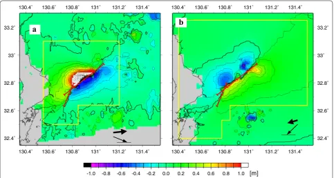
Beppu–Shimabara graben (Tada 1984), where north– south extension is dominant, and the major shear zone in Kyusyu detected by Matsumoto et al. (2015), where east– west compression is important as well as north–south extension. The aftershock activity and InSAR data (Fig. 2) also support that the fault rupture occurred mainly along the Futagawa fault, but the Hinagu fault moved, too. Cen-troid moment tensor (CMT) solution determined by the Global CMT Project (Ekström et al. 2012) shows that the earthquake (Mw 7.0) has a significant nondouble-couple component, which cannot be explained by slips on a sin-gle flat plane.
The geometry of an inland active fault is often not well constrained; even if a clear fault trace has been observed, it is not easy to well constrain the dip angle of it. In the case of the Kumamoto earthquake, vigorous aftershocks
Open Access
*Correspondence: [email protected]
are spatially distributed and do not clearly align on fault planes (the JMA unified earthquake catalog). For a large earthquake in a remote area, it is more difficult to determine the fault dip angle because of the poor deter-mination of the location of seismicity. When we can-not constrain the fault geometry, the inversion analysis to estimate the slip distribution on the fault becomes nonlinear. In such a case, the dip angle has often been obtained by minimizing the square misfit under the assumption of a uniform slip on a rectangular fault (e.g.,
Árnadóttir and Segall 1994; Wright et al. 2003; Schmidt and Bürgmann 2006). It is not guaranteed, however, that the dip angle determined under the assumption of a uni-form slip gives the best estimate for a spatially variable slip distribution.
In such situations, synthetic aperture radar interferom-etry (InSAR) data give valuable information in estimating fault slip distribution as well as fault geometry, because they can provide spatially very dense crustal displace-ment data even in a remote area, where the coverage of
Global Navigation Satellite System (GNSS) and seismic networks is sparse. In May 2014, the Japan Aerospace Exploration Agency (JAXA) launched Advanced Land Observation Satellite 2 (ALOS-2) that equipped Phased Array type L-band Synthetic Aperture Radar 2 (PAL-SAR-2). ALOS-2 can acquire images with a much shorter interval than the previous satellite (ALOS-1), owing to a shorter recurrence interval (14 days) of the satellite orbit and a wider look angle (a ScanSAR mode). ALOS-2 can also make observation in both right and left directions, which enhances the opportunities to obtain different line-of-sight (LOS) displacements. Because of that, it has become much easier to obtain InSAR images with differ-ent LOS displacemdiffer-ent vectors soon after a large earth-quake, which significantly reduces the contamination of postseismic deformation.
As mentioned above, at least two faults moved in the case of the Kumamoto earthquake. In general, slip on a fault affects the estimate of the slip on another fault in the inversion analysis. So, we must simultaneously solve this complicated inverse problem. The nonlinearity of the inverse problem, however, is still not significant, when we can assume a flat fault plane for each fault. The unknown parameters that cause nonlinearity are only the
dip angles of the two faults owing to relatively clear fault traces. So, in this study, we extend the method of Fuka-hata and Wright (2008) for the case of a two-fault system. With the method of Fukahata and Wright (2008), we can simultaneously determine the optimal dip angle of a fault and the slip distribution on it, based on Akaike’s Bayes-ian information criterion (ABIC) by regarding the dip angle as a hyperparameter. The method has been applied to several earthquakes, such as the 1995 Dinar, Turkey (Fukahata and Wright 2008), the 2008 Wenchuan, China (Enomoto et al. 2010), the 2008 Iwate-Miyagi nairiku, Japan (Fukahata 2009), and the 2010 Haiti (Hashimoto et al. 2011). If this extension has success, the method becomes a powerful tool in clarifying the slip distribu-tion, even though a complicated rupture like the Kuma-moto earthquake occurred in a remote area with sparse GNSS and seismic networks.
Inversion method
For the problem to estimate slip distribution of an earth-quake, when the fault geometry is unknown, as stated above, the inverse problem is nonlinear. In this case, the observation equation that relates data d to model param-eters m is written in the following form:
130.4˚ 130.4˚
130.6˚ 130.6˚
130.8˚ 130.8˚
131˚ 131˚
131.2˚ 131.2˚
131.4˚ 131.4˚
32.4˚ 32.6˚ 32.8˚ 33˚
33.2˚
a
130.4˚ 130.4˚
130.6˚ 130.6˚
130.8˚ 130.8˚
131˚ 131˚
131.2˚ 131.2˚
131.4˚ 131.4˚
32.4˚ 32.6˚ 32.8˚ 33˚ 33.2˚
-1.0 -0.8 -0.6 -0.4 -0.2 0.0 0.2 0.4 0.6 0.8 1.0
b
[m]
f is a vector of a nonlinear function of m and includes Green’s function that gives surface displacement for a given slip in an elastic half-space. m consists of the parameters that represent the fault geometry p and the fault slip distribution a. e is error that consists of obser-vation and modeling errors. Because the inverse problem becomes linear for a given fault geometry, Eq. (1) can be rewritten as
where H is a N×M matrix that depends on p; N and M are the number of data and the number of model param-eters excluding p, respectively. Because we consider that slip occurs on two flat faults and that only the dip angle
δi (i = 1, 2) of each fault is unknown among the fault parameters p, we can express Eq. (2) as
where ai represents the slip distribution on ith fault and
Hi are the corresponding coefficient matrix.
We also use smoothness condition as a prior con-straint. The smoothness condition should be applied to slip distribution on each fault; then, the roughness r, through which the smoothness is defined, is written in the following form:
where Gi is a Mi×Mi matrix that represents the
smooth-ness condition, and Mi is the number of model
param-eters ai.
Using newly defined H, G, and a, we can obtain the expression of ABIC in the same form as eq. (20) of Fuka-hata and Wright (2008). Here, as mentioned above, we treat the dip angles, δ1 and δ2, as hyperparameters like the weight of smoothing. The weight of smoothing is also taken in the same way as in Fukahata and Wright (2008). The values of δ1, δ2 and the smoothing parame-ter that give ABIC minimum are adopted as the optimal ones (Akaike 1980). In the search of the global minimum of ABIC that is a function of δ1, δ2 and the smoothing parameter, we first take a coarse grid that spans a very
(1)
wide range of these parameters, and then change the grid intervals finer and finer around the ABIC minimum. Once, we obtain the optimal values of the dip angles and smoothing parameter, we can obtain the optimal values of the usual model parameters a that give slip distribu-tion on the faults by a usual linear inversion (Yabuki and Matsu’ura 1992; Fukahata and Wright 2008).
InSAR data
JAXA is operating a satellite ALOS-2 that equipped PALSAR-2, which is a L-band SAR emitting microwave of the wavelength of 23.6 cm. Because L-band SAR has a capability to penetrate to the ground through heavy vegetation, we can expect high coherence. We collected ALOS-2/PALSAR-2 images acquired before and after the Kumamoto earthquake sequence. We applied two-pass differential interferometry to available pairs of images with Gamma® software with ASTER GDEM ver. 2 (Tachi-kawa et al. 2011) and obtained interferograms. All inter-ferograms were flattened to reduce errors and unwrapped using the branch-cut algorithm. In this paper, we use interferograms of ScanSAR images acquired with right (path 135–650; Fig. 2a) and left (path 124–700; Fig. 2b) looking from ascending orbits, because these images cover the entire source region and give us different view of deformation from both east and west. The detailed information on the statistics of ALOS-2/PALSAR-2 Scan-SAR images used in this study is given in Table 1. Note that these InSAR data include the displacement due to not only the main shock (Mw 7.0) but also other sources including the largest foreshock (Mw 6.2).
These InSAR data images show large discontinuities in LOS displacement along the Futagawa fault. The right-looking image (Fig. 2a) shows that the south side of the fault moves to the satellite and the north side of the fault moves away from the satellite. The difference in LOS displacement amounts to 2.6 m. The left-looking image (Fig. 2b) shows mostly the opposite motion, but the amplitude of the LOS displacement is much smaller. This means that the fault slip motion is mainly right lateral, but with significant vertical slip components; the north block subsides and the south block uplifts. We can also see clear difference in displace-ments across the Hinagu fault, which is consistent with the findings of surface rupture along the northernmost part of it. Surface displacement in Aso caldera is also significant, particularly in the southwestern part.
Table 1 Statistic of ALOS-2/PALSAR-2 ScanSAR images used in this study
Path/frame Pre-event acquisition Postevent acquisition Perpendicular baseline (m) Heading (°) Incidence angle (°)
Many local surface deformations possibly related to landslides were induced by the Kumamoto earthquake. These local movements often cause loss of coherence. Therefore, we excluded such areas during unwrapping from InSAR data images, but this trial was not per-fect. So, in the inversion analysis, we only used the data enclosed by the yellow lines in Fig. 2a, b to reduce the effect of the contamination of signals related to landslides and other error sources.
We subsample the InSAR data using quadtree algo-rithm (Jónsson et al. 2002). The minimum and maximum block sizes are about 700 m and 5 km, respectively. The total number of data used in the inversion analysis is about 1900 for the image of Fig. 2a and about 1000 for Fig. 2b. Because InSAR data commonly have spatially well-correlated errors, we take the covariance compo-nents of InSAR data into account in the same way as in Fukahata and Wright (2008). That is, we assume that the covariance components exponentially decrease with the distance between InSAR data points.
Results
By referring to the observed surface ruptures as well as the InSAR images, we set the surface traces of the two faults as shown in Figs. 1 and 2. The strikes of the Fut-agawa and Hinagu faults are taken to be 232° and 203°, respectively. The length of the Futagawa and Hinagu faults is 40 and 20 km, respectively, and the depth of the faults is 16 km. Because of intensive surface deformation, we do not use the InSAR data within about 2 km from the model fault traces. We focus on the broad feature of fault slip distribution by neglecting very complicated deformation near the fault traces. As for basis functions, we use bicubic B-splines with an interval of 2 km in both (horizontal and depth) directions. In the computation of Green’s function, we assume a homogenous elastic half-space of a Poisson solid with a rigidity of 3.43 × 10¹⁰ Pa.
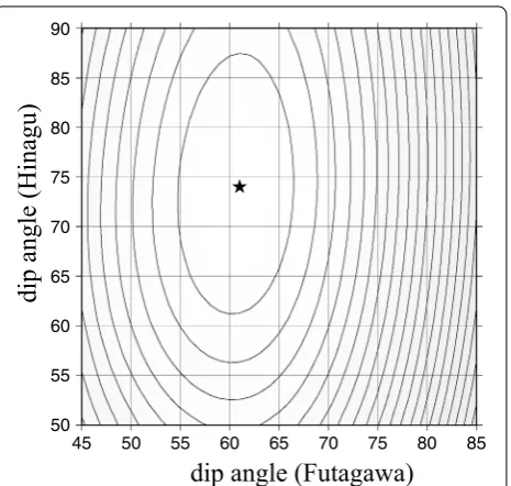
Under this condition, we compute the values of ABIC and plot them in a contour map with a contour interval of 2 in ABIC (Fig. 3). The point of the ABIC minimum, shown by the star, gives the best estimates for the dip angles of the Futagawa and Hinagu faults. Because the difference of one free hyperparameter corresponds to 2 in the value of ABIC (Akaike 1980), a difference of 2 in ABIC has statistical significance. So, the dip angles are estimated to be 61° ± 6° for the Futagawa fault and 74° ± 12° for the Hinagu fault. The mutual depend-ence on these estimates is very weak, as shown in Fig. 3. Hence, at least in this case, we find that the dip angles can be almost independently determined. The value of ABIC also depends on another hyperparameter, the weight of smoothing. In this case, fortunately, we also find that the mutual dependence of the dip angles on the weight
of smoothing is very weak. In the overall range shown in Fig. 3, the optimal value of the smoothing parameter has nearly the same value. The standard deviation of the data error e for the optimal model is about 12 cm.
Figure 4 shows the slip distribution for the optimum ABIC value. The largest slip on the Futagawa fault is over 5 m around the center of the model fault, which is 130.9° in longitude at the Nishihara village. The slip on the Futagawa fault is mainly strike slip, but with a signifi-cant normal slip component that exceeds 3 m around the area of the largest slip. This feature is well consistent with the InSAR data; around the center of the model fault, the shortening of the LOS displacement in the north side of the Futagawa fault in Fig. 2b is much smaller than the neighboring areas along the fault, which is considered to be due to large subsidence in this area. The slip on the Hinagu fault is almost a pure strike slip with a peak of about 2.4 m. The total moment release of the earthquake is estimated to be 4.4 × 10¹⁹ N m. The contribution of the
Hinagu fault is about 20% of it. Thus, from the difference of the moment magnitudes between the largest foreshock (Mw 6.2) and the main shock (Mw 7.0), about one-third of the estimated slip on the Hinagu fault (Fig. 4) would be caused by the largest foreshock.
The slip on the Futagawa fault quickly decreases to zero beyond the intersection with the Hinagu fault. On the other hand, Aso caldera does not have such an effect. The model Futagawa fault intersects with Aso caldera about
−10 km in the horizontal distance. Just inside of Aso
50
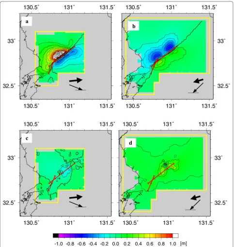
caldera, we can see a local peak of the surface displace-ment. This would be a cause of severe damage in this area. Given the slip distribution (Fig. 4), we can calculate the LOS crustal displacements for the right (Fig. 5a)- and left (Fig. 5b)-looking images. By subtracting the model crustal displacements (Fig. 5a, b) from the observed data (Fig. 2a, b), the residual LOS crustal displacements are obtained (Fig. 5c, d). The residual is mostly smaller than 10 cm that is <1 fringe in the original InSAR data, except for the area near the caldera rim of Aso volcano, where the misfit amounts to 30 cm.
Discussion and conclusions
In the inversion scheme used in this paper, we do not apply the nonnegative condition for slip, because the emergence of negative slip is a good indicator of the goodness in the setting of inversion analysis (Fukahata and Wright 2008; Yagi and Fukahata 2011). In this study, the negative slip corresponds to a left lateral slip and a reverse fault slip. In Fig. 6a, we show a result of slip inversion for the case of only one (Futagawa) fault, instead of a two-fault sys-tem. The slip distribution (Fig. 6a) is fairly similar to the one for the two-fault model (the left diagram of Fig. 4), but we can see a significant negative (reverse fault) slip on the southwestern part of the fault (Fig. 6b). The negative dip slip amounts to about 70 cm, although the strike slip does not have a negative slip component (Fig. 6c). In this inver-sion analysis, we used the same dip angle and smoothing
parameter as the optimal values of the two-fault model. When we use the optimal values in this fault setting, we obtain larger negative slips. On the other hand, when we add the Hinagu fault to the model, we find that the nega-tive slip on the southwestern part of the fault almost completely vanishes away (Fig. 6d). This means that the combination of the Futagawa and Hinagu faults is neces-sary in the inversion analysis of the 2016 Kumamoto earth-quake. In fact, the residuals for the one-fault model are significantly larger near the Hinagu fault (Additional file 1: Figure S1), which was neglected in the one-fault model.
On the other hand, the northeastern part of the Futa-gawa fault has another significant negative slip even for the case of the two faults (Fig. 6d), which well coincides with a relatively large misfit area in the InSAR data (Fig. 5c, d). These things suggest that something is wrong in the set-ting of the inversion. However, we have not been able to find the solution of this problem. For example, linearly distributed surface ruptures were found in the northwest-ern part of Aso caldera (Geospatial Information Author-ity of Japan 2016; Lin et al. 2016). So, we put another fault there, but we still obtained significant negative slips (Additional file 1: Figure S2). The result suggests that the surface ruptures found in the northwestern part of Aso caldera are what we call nontectonic faults and they are unlikely to have a deeper root. We also tried various cases by putting another fault in this area and calculated the slip distribution, but it was difficult to drastically reduce the 0
negative slip as in the southwestern part. More compli-cated fault geometry, curved and/or more than one fault, may be needed. Otherwise, because the negative slip area coincides with the caldera rim of Aso volcano, something
peculiar might happen, due to mass wasting, loose sedi-ment, and/or large contrast of the elastic constants.
We also tried to use pixel offset data, range, and azimuth offsets, of path 23 and path 28 obtained by
130.5˚
130.5˚
131˚
131˚
131.5˚
131.5˚
32.5˚
33˚
a
130.5˚
130.5˚
131˚
131˚
131.5˚
131.5˚
32.5˚
33˚
b
130.5˚
130.5˚
131˚
131˚
131.5˚
131.5˚
32.5˚
33˚
c
130.5˚
130.5˚
131˚
131˚
131.5˚
131.5˚
32.5˚
33˚
-1.0 -0.8 -0.6 -0.4 -0.2 0.0 0.2 0.4 0.6 0.8 1.0
d
[m]
ALOS-2/PALSAR-2. The former is collected on March 7, 2016, and April 18, 2016, and the latter is collected on November 14, 2014, and April 29, 2016. The range offsets are mostly consistent with InSAR data used in this study, though look angles are slightly different, while azimuth offsets give nearly the north–south com-ponent of displacement. By inverting the range and azimuth offset data together with the InSAR data, we obtained a similar result with slightly larger amplitude in slip. However, the result also has more negative slips probably due to larger error, mainly due to inaccurate orbit, included in the pixel offset data. Because of that we avoided to use the pixel offset data in the inversion analysis of this study.
We did not use GNSS data in the inversion analysis, because our primal objective is to develop a method that can be used for a remote area, where dense GNSS and seismic networks are unavailable. We compare the synthetic displacement computed from the slip model (Fig. 4) with observed GNSS data in Additional file 1: Figure S3. Although we can see significant discrepancy at some places, local effects may also be important. For example, the blue vectors for vertical displacements show larger subsidence than the synthetic, but all the points are situated on the sedimentary layer, and so compac-tion might be induced by the shaking of the earthquake. Kamai (2016) also reports that a branch fault that moved at the 2016 Kumamoto earthquake passes through near
0
Futagawa only (1 fault model)
0.5
d Dip Slip (2 fault model)
-0.7
e Strike Slip (2 fault model)
0.5
3. 5 4
by Choyo station (Green’s vectors), which must signifi-cantly affect the displacement there. Considering that the GNSS data are not used in the inversion analysis, the fit-ting to GNSS data (Additional file 1: Figure S3) is not bad. Although there are the problems of negative slip and large misfit around the caldera rim, our solution looks over-all reasonable (almost no negative slip) and the misfit is also small. InSAR data are well inverted to slip on the Futagawa and Hinagu faults. So, with the method developed in this study, we can reasonably estimate the slip distribution on faults for an earthquake that ruptures more than one fault in a remote area. In general, InSAR data better constrain total slip distribution on a fault than seismic data (Funning et al. 2014), because usually seismic data are directly related to slip velocities or accelerations on the fault, which must then be integrated in order to obtain slip amount, although seismic data have the ability to clarify the rupture process of an earthquake. For example, the resolution of Yagi et al. (2016) and Asano and Iwata (2016), who used teleseismic P-wave data and near-field strong motion data, respectively, seems to be not enough, although the latter well detected the largest slip area with significant normal slip compo-nents around the center of the Futagawa fault. On the other hand, the shape of the large slip area of Kubo et al. (2016), which becomes shallower from the center of the Futagawa fault to the northeast with little slip below there, is consist-ent with the slip distribution of this study.
Authors’ contributions
YF designed this study, carried out the inversion analysis, and prepared the manuscript. MH analyzed the SAR images. Both authors read and approved the final manuscript.
Acknowledgements
We thank Haruo Horikawa and anonymous reviewers for useful comments. ALOS-2/PALSAR-2 images were provided by JAXA through the Earthquake SAR Working Group (Secretariat: the Geospatial Information Authority). The copy-right and the ownership belong to JAXA. The JMA unified earthquake catalog is produced by JMA in cooperation with the Ministry of Education, Culture, Sports, Science and Technology (MEXT). The GEONET data are provided by the Geospatial Information Authority of Japan. Figures were created with the GMT software by Paul Wessel and Walter H. F. Smith. This study was partly supported by MEXT KAKENHI Grant Nos. 16K05539, 26109001, and 26109003 to YF.
Competing interests
Both authors declare that they have no competing interests.
Received: 1 August 2016 Accepted: 29 November 2016
References
Akaike H (1980) Likelihood and the Bayes procedure. In: Bernardo JM, DeGroot MH, Lindley DV, Smith AFM (eds) Bayesian statistics. University Press, Valencia, pp 143–166
Árnadóttir T, Segall P (1994) The 1989 Loma Prieta earthquake imaged from inversion of geodetic data. J Geophys Res 99:21835–21855
Asano K, Iwata T (2016) Source rupture processes of the foreshock and main-shock in the 2016 Kumamoto earthquake sequence estimated from the kinematic waveform inversion of strong motion data. Earth Planets Space 68:147. doi:10.1186/s40623-016-0519-9
Ekström G, Nettles M, Dziewonski AM (2012) The Global CMT Project 2004–2010: centroid-moment tensors for 13,017 earthquakes. Phys Earth Planet Inter 200–201:1–9
Enomoto M, Hashimoto M, Fukushima Y, Fukahata Y (2010) Analysis of crustal deformation associated with the 2008 Wenchuan, China, Earthquake using ALOS/PALSAR data. J Geod Soc Jpn 56:155–167 (in Japanese with English abstract)
Fukahata Y (2009) Crustal displacements and inversion analysis for slip distri-bution on 2008 Iwate-Miyagi nairiku earthquake, vol 52. Disaster Preven-tion Research Institute Annuals, Kyoto University, Kyoto, pp 131–137 (in Japanese with English abstract)
Fukahata Y, Wright TJ (2008) A non-linear geodetic data inversion using ABIC for slip distribution on a fault with an unknown dip angle. Geophys J Int 173:353–364
Funning G, Fukahata Y, Yagi Y, Parsons B (2014) A method for the joint inversion of geodetic and seismic waveform data using ABIC: application to the 1997 Manyi, Tibet, earthquake. Geophys J Int 196:1564–1579 Geospatial Information Authority of Japan (2016) Information on the 2016
Kumamoto Earthquake. http://www.gsi.go.jp/BOUSAI/H27-kumamoto-earthquake-index.html#dd. Accessed 13 July 2016
Hashimoto M, Fukushima Y, Fukahata Y (2011) Fan-delta uplift and mountain subsidence during the Haiti 2010 earthquake. Nat Geosci 4:255–259 Jónsson S, Zebker H, Segall P, Amelung F (2002) Fault slip distribution of the
1999 Mw 7.1 Hector Mine, California, earthquake, estimated from satellite radar and GPS measurements. Bull Seismol Soc Am 92:1377–1389 Kamai T (2016) Landslide hazards induced by the 2016 Kumamoto earthquake.
Bull Jpn Assoc Earthq Eng 29:27–32 (in Japanese)
Kubo H, Suzuki W, Aoi S, Sekiguchi H (2016) Source rupture processes of the 2016 Kumamoto, Japan, earthquakes estimated from strong-motion waveforms. Earth Planets Space 68:161. doi:10.1186/s40623-016-0536-8 Matsumoto S, Nakao S, Ohkura T, Miyazaki M, Shimizu H, Abe Y (2015) Spatial
heterogeneities in tectonic stress in Kyushu, Japan and their rela-tion to a major shear zone. Earth Planets Space 67:172. doi:10.1186/ s40623-015-0342-8
Additional file
Research group for active faults of Japan (1991) Active faults in Japan. Sheet maps and inventories, revised edn. University of Tokyo Press, Tokyo Schmidt DA, Bürgmann R (2006) InSAR constraints on the source parameters of the
2001 Bhuj earthquake. Geophys Res Let 33:L02315. doi:10.1029/2005GL025109 Sibert L, Simkin T (2002) Volcanoes of the world: an illustrated catalog of
Holocene volcanoes and their eruptions. Smithsonian Institution Digital Information Series GVP-3. http://www.volcano.si.edu/gvp/world Tachikawa T, Hato M, Kaku M, Iwasaki A (2011) The characteristics of ASTER
GDEM version 2, presented in IGARSS, July 2011
Tada T (1984) Spreading of the Okinawa trough and its relation to the crustal deformation in Kyusyu. Zisin-2 37:407–415 (in Japanese with English abstract)
Wessel P, Smith WHF (1998) New, improved version of generic mapping tools released. EOS Trans Am Geophys Union 79:579. doi:10.1029/98EO00426
Wright TJ, Lu Z, Wicks C (2003) Source model for the Mw 6.7, 23 October 2002, Nenana Mountain Earthquake (Alaska) from InSAR. Geophys Res Lett 30:1974. doi:10.1029/2003GL018014
Yabuki T, Matsu’ura M (1992) Geodetic data inversion using a Bayesian information criterion for spatial distribution of fault slip. Geophys J Int 109:363–375
Yagi Y, Fukahata Y (2011) Introduction of uncertainty of Green’s function into waveform inversion for seismic source processes. Geophys J Int 186:711–720