7-10-2014 12:00 AM The Influence of Microstructure on the Corrosion of Magnesium Alloys

(1)

Scholarship@Western

Electronic Thesis and Dissertation Repository

7-10-2014 12:00 AM

The Influence of Microstructure on the Corrosion of Magnesium

Alloys

Robert M. Asmussen

The University of Western Ontario Supervisor

Dr. David Shoesmith

The University of Western Ontario Graduate Program in Chemistry

A thesis submitted in partial fulfillment of the requirements for the degree in Doctor of Philosophy

Follow this and additional works at: https://ir.lib.uwo.ca/etd

Part of the Analytical Chemistry Commons, and the Materials Chemistry Commons

Recommended Citation Recommended Citation

Asmussen, Robert M., "The Influence of Microstructure on the Corrosion of Magnesium Alloys" (2014). Electronic Thesis and Dissertation Repository. 2134.

https://ir.lib.uwo.ca/etd/2134

This Dissertation/Thesis is brought to you for free and open access by Scholarship@Western. It has been accepted for inclusion in Electronic Thesis and Dissertation Repository by an authorized administrator of

(2)

i

OF MAGNESIUM ALLOYS

(Thesis format: Integrated Article)

by

R. Matthew Asmussen

Graduate Program in Chemistry

A thesis submitted in partial fulfillment of the requirements for the degree of

Doctor of Philosophy

School of Graduate and Postdoctoral Studies Western University

London, Ontario, Canada

(3)

ii

This thesis reports a series of investigations into the influence of microstructure

on the corrosion of Mg alloys. Mg alloys are prime candidates for the light-weighting of

automobiles however any extensive applications are limited by their high corrosion rates.

The corrosion resistance is further hindered by the susceptibility of Mg alloys to

microgalvanic coupling occurring between the Mg matrix and the secondary

microstructures in the alloys. This process and the individual contributions to it must be

understood to improve Mg alloy design for automotive applications, develop methods for

extending the lifetime of Mg alloys and developing models to successfully predict the

corrosion behaviour of Mg alloys.

An experimental procedure for tracking corrosion on lightweight alloys has been

developed using a combination of microscopy and corrosion studies using commercial

sand cast magnesium AM50 alloys. Corrosion penetration depths were measured and

characterized with CLSM and SEM/XEDS, respectively. Corrosion depths on α-grains

in the alloys were expressed as a function of their Al content. Al-rich β-phases and

eutectic α-phase microstructures were observed to be most corrosion resistant due to an

enrichment of Al, identified with TEM, near the oxide/alloy interface. Sand cast alloys

were found to be susceptible to major corrosion events in regions with depleted Al

content.

The corrosion of sand, graphite and die cast Mg AM50 alloy were compared in

1.6 wt% NaCl solution to determine the influence of microstructure size and distribution

of Al. The differences in corrosion mechanism were determined using electrochemical

(4)

iii

The corrosion performance improved in the order sand cast < graphite cast < die cast.

This was shown to be due to the increasing tightness of the α-Mg/β-phase/Al-containing

microstructural network, which lead to an increased protection of the surface by

Al-enriched eutectic and a decrease in the probability of initiating a major damage site on an

α-Mg region with low Al content.

Al-Mn intermetallic particles are active cathodes in the microgalvanically-coupled

corrosion of Mg alloys. Domes of corrosion product, mainly Mg(OH)2, collect on the

particles as corrosion proceeds. The electrochemical behaviour (corrosion potential,

potentiodynamic polarization, and potentiostatic measurements) of two Al-Mn

intermetallic materials (Al- 11 wt% Mn and Al-25 wt% Mn) has been studied in 0.275 M

NaCl and 0.138 M MgCl2 solutions to simulate the cathodic behaviour of Al-Mn particles

during the corrosion of a Mg alloy. Following a 20 h polarization at -1.55 V (vs. SCE),

the Al-Mn intermetallic suffered dealloying of Al and the growth of Al hydroxide and

Mn-oxide containing surface layers. A similar electrochemical treatment in MgCl2

solution lead to the accumulation of a Mg(OH)2 layer on the alloy surface which lowers

cathodic reactivity and partially protects the intermetallic from dealloying. This

electrochemical simulation of behaviour experienced on the microscale by Al-Mn

intermetallics on corroding Mg alloys confirms the appearance of corrosion product

domes on Al-Mn intermetallics during the corrosion of Mg alloys is an indication of their

cathodic behaviour.

The corrosion behaviour of Mg alloy ZEK100 was investigated in water and in

(5)

iv

phases. Potentiodynamic polarization measurements showed the corrosion resistance of

the ZEK100 improved with decreasing chloride content. Intermittent immersions in

0.16 wt% NaCl showed corrosion occurred preferentially along grain boundaries

interlinking the secondary phase particles some of which acted as active cathodes

microgalvanically-coupled to the α-Mg matrix. This grain boundary sensitivity appeared

to be a consequence of the depletion of the alloying elements, especially Zn, at these

locations. Of the three types of secondary phase identified, T-phase, Zr and

Fe-containing Zr particles, the latter were the dominant active cathodes. This was

demonstrated by experiments in pure water when grain boundary corrosion was avoided

and active cathodes could be identified by a small surrounding zone of corroded α-Mg

and an accumulated dome of corrosion product on the active particle.

The suppression of the corrosion of AM50 Mg alloys in NaCl solutions was

investigated using galvanic coupling and chronopotentiometric techniques. When

galvanically coupled to pure Mg, sand, graphite and die cast AM50 alloys yielded a net

cathodic current between -15 µA/cm2 and -30 µA/cm2, and limited corrosion damage was

observed on the coupled surfaces compared with uncoupled surfaces. This protective

effect was artificially simulated chronopotentiometrically by applying cathodic current to

the die cast AM50 alloy. Current densities as low as -0.1 µA/cm2 were found to resist the

initiation of extensive corrosion. This effect is attributed to the ability of the applied

current to satisfy the cathodic demand for current at microstructural features such as

Al-Mn intermetallics leading to a temporary decoupling of the microgalvanic linkage

(6)

v

containing 3 mM NaCl using a range of electrochemical techniques including

electrochemical impedance spectroscopy and scanning electrochemical microscopy.

Scanning electron microscopy and energy dispersive X-ray analyses were used to locate

and elementally analyze the microstructural features of the alloy and to locate and

correlate their relationship to SECM mapping. Confocal scanning laser microscopy was

used to observe the nature and distribution of corrosion damage. By switching from an

aqueous corrosion medium to ethylene glycol, it was shown that the corrosion of sand

cast AM50 alloy was significantly suppressed thereby quenching H2 evolution. The

corrosion activity of the AM50 alloy was mapped using the feedback mode of scanning

electrochemical microscopy. Ferrocenemethanol, serving as a redox mediator, can be

used as a cathodic site contrasting agent exposing the reactive anodic areas of the

corroding surface. These studies confirmed that the corrosion mechanism of Mg is the

same in ethylene glycol as it is in water, and that studies in this solvent can be used to

elucidate the reaction features obscured by rapid corrosion in water.

This thesis provides an essential contribution to the understanding of the

microscaled corrosion of Mg alloys. The methodology developed can be further applied

to a wide range of Mg alloys to investigate their behaviour. An ex-situ identifier of

cathodic activity, a corrosion product dome, was confirmed; allowing for ease of

identification of microgalvanic cathodes in future investigations. New approaches to

controlling the corrosion rate of Mg alloys were also reported involving the application of

(7)

vi

(8)

vii

This thesis contains published data. For the work I was the lead investigator and

writer and performed the experimental portions with assistance from:

Chapter 3 P. Jakupi assisted with CLSM experimental design, M. Danaie performed

TEM analysis, G. Botton and D. Shoesmith assisted with editing.

Chapter 4: W. Binns assisted with electrochemical measurements, P. Jakupi and D.

Shoesmith with editing.

Chapter 5: R. Partovi-Nia performed XRD analyses, W. Binns, P. Jakupi and D.

Shoesmith assisted with editing.

Chapter 6 : W. Binns, P. Jakupi and D. Shoesmith assisted with editing.

Chapter 8: W. Binns assisted with electrochemical measurements, SECM was performed

at McGill University by P. Dauphin Ducharme and U. M. Tafashe, J. Mauzeroll, P.

(9)

viii

This thesis would not have been remotely possible without the guidance and

support of my supervisor, Dr. Dave Shoesmith. His mentorship allowed me to grow as a

researcher and made my doctoral studies a fully enjoyable experience. I can’t begin to

express my gratitude in words for the opportunities granted and example set by him

throughout the past 3.5 years. The only way of saying thanks is to take the lessons learnt

from him, in research and life, and continue applying them throughout my career. That,

of course, does not include choice of pro-sports teams to back

The members of the Shoesmith group, past and present, made my time in the lab

productive and highly enjoyable. Specifically, Dr. Pellumb Jakupi who has been a part of

this Mg project since its launch in May 2011 has been an invaluable co-worker and

friend. It was not only corrosion knowledge I gained from working with him, but mainly

the importance of selling yourself and your research to the scientific community and the

importance of going just for one. Jeff Binns, whose introduction to this project coincided

directly with its rapid growth, despite sometimes ruining our aura of success with a

Canadiens hat. Dr. Jian Chen for being a great friend to have in the work place and also

the greatest resource of knowledge I had at my disposal during this time, even when he

had “just one question for me”. Dr. Jaime Noel (old-clyde, new-clyde, nuclide), Dr.

Dmitrij Zagidulin, and Dr. Zack Qin for their contributions, assistance and considerable

knowledge during the term of my thesis.

I must thank my collaborators on this project: Dr. Gianluigi Botton and Dr.

Mohsen Danaie from the Canadian Centre for Electron Microscopy at MacMaster

(10)

ix

stints at both universities during the previous three years.

I owe an indescribable amount of gratitude to my parents, Kim and Brenda

Asmussen, who never pushed or pressured me, let me choose my own path and have been

nothing but supportive along the way. I attribute my successes, both previous and in the

future, to the values and work ethic they have provided me. My siblings, Mike and Nerd,

for the support they offer and friendship I can always count on from both of them. And

to all my friends near and far, for the good times, the bad times and that one time…..

For her love, encouragement and witty bant…..ah who am I kidding, to Susan for

being the best addition to my life and always reminding me no matter how tough things

got, it was probably worse in Petawawa.

And for their contributions to my sanity over the past couple of years, I would like

to thank the makers of great craft beer everywhere, Hot Italian Sandwiches, Shmokey

Rob’s, smooth (and needed) drams of scotch, DDP Yoga and the country roads around

(11)

x

This thesis is dedicated to my two biggest supporters,

The two men whom I try to mold myself after every day of my life,

The two men who instilled my character and drive,

And the two men who I wish were here to see this achievement,

(12)

xi

Abstract ... ii

Co-authorship Statement ... vii

Acknowledgements ... viiii

Table of Contents ... xi

List of Symbols and Acronyms ... xix

List of Tables ... xxii

List of Figures ... xxiiii

Chapter One - Introduction ... 1

1.1 Introduction ... 1

1.2 Magnesium and its Alloys ... 7

1.3 Aqueous Corrosion ... 10

1.3.1 Thermodynamics of Corrosion ... 10

1.3.2 Kinetics of Corrosion ... 16

1.4 Corrosion of Magnesium and its Alloys ... 22

1.4.1 Corrosion of Mg ... 22

1.4.2 The Corroding Surface of Mg and its Alloys ... 24

1.4.3 Magnesium’s Great White Buffalo: The Negative Difference Effect and Mg+ .... 26

(13)

xii

1.4.5.1 Aluminum ... 30

1.4.5.2 Other Alloying Elements ... 31

1.4.6 Corrosion Behaviour of Mg Alloys ... 33

1.4.7 Microstructural Effects on Corrosion ... 35

1.4.7.1 Grain Size ... 36

1.4.7.2. Al-Mn Intermetallics ... 37

1.4.7.3 β-phase ... 37

1.5 Scope of Thesis ... 39

1.6 References ... 41

Chapter Two - Experimental: ... 55

2.1 Microscopy ... 55

2.1.1 Scanning Electron Microscopy (SEM)... 55

2.1.1.1 Instrumentation ... 55

2.1.1.2 SEM Experimental Details ... 57

2.1.2 Focused Ion Beam (FIB) ... 59

2.1.3 Confocal Laser Scanning Microscopy (CLSM) ... 60

2.1.3.1 Instrumentation ... 60

2.1.4 Transmission Electron Microscopy (TEM) ... 62

(14)

xiii

2.2 Sample Preparation ... 63

2.3 Intermittent Immersion Experiments ... 66

2.4 Chromium Treatment of Mg Alloys ... 68

2.5 Electrochemistry ... 70

2.5.1 Electrochemical Measurements ... 70

2.5.2 Electrochemical Impedance Spectroscopy (EIS) ... 72

2.5.3 EIS Experimental Details ... 75

Chapter Three – Tracking the Corrosion of Sand Cast AM50 Mg Alloys in Chloride Environments ... 79

3.2 Experimental ... 80

3.2.1 Sample Preparation ... 80

3.2.2 Instrumentation ... 81

3.2.3 Tracking Corrosion on the Microscale ... 82

3.2.4 Surface Montage Imaging ... 82

3.3 Results ... 83

3.3.1 Corrosion Behaviour of Sand Cast AM50 Alloys in 1.6 wt. % NaCl... 83

(15)

xiv

3.4 Discussion ... 101

3.5 Summay and Conclusions ... 102

Chapter Four – The Microstructural Effects on Corrosion of AM50 Magnesium Alloys ... 106

4.2.1 Sample Preparation ... 107

4.2.2 Instrumentation ... 108

4.2.3 Intermittent Immersion Experiments ... 109

4.2.4 Electrochemical Analysis... 110

4.3 Results ... 111

4.3.1 Alloy Characterization ... 111

4.3.2 Electrochemical Behaviour ... 115

4.3.3 Corrosion Behaviour in 1.6 wt. % NaCl ... 118

4.5 Summary and Conclusions ... 127

(16)

xv

The Behanviour of Al-Mn Alloys in NaCl and MgCl2 ... 133

5.2.1 Materials ... 135

5.2.3 Surface Analysis ... 136

5.3 Results ... 137

5.3.1 Al-Mn Intermetallics ... 137

5.3.3 Surface Behaviour ... 143

Chapter Six – The Influence of Microstructure on the Corrosion of Mg Alloy ZEK100 ... 162

(17)

xvi

6.2.4 Intermittent Immersion Experiments... 165

6.3 Results ... 165

6.3.1 Surface Imaging ... 165

6.3.2 Electrochemical Effect of Chloride Ion Concentration ... 168

6.3.3 Intermittent Immersions in Chloride Solutions ... 168

6.3.4 Intermittent Immersions in Pure Water ... 181

Chapter Seven – Sacrifical Anode and Cathodic Protection of Mg Alloys ... 196

7.2. Experimental ... 197

7.2.2 Microscopy ... 198

7.2.3 Galvanic Coupling Experiments ... 198

7.2.4 Galvanostatic Control ... 198

7.3 Results ... 199

7.3.1 AM50 Alloy Coupled to Pure Mg... 199

(18)

xvii

Chapter Eight – Reducing the Corrosion Rate of Mg Alloys Using Ethylene Glycol for Advanced Elctrochemical Imaging ... 220

8.2.1 Materials ... 221

8.2.4 Electron Microscopy ... 223

8.2.5 Scanning Electrochemical Microscopy (SECM) ... 223

8.3 Results ... 224

8.3.1 AM50 Alloy Microstructure ... 224

8.3.3 Corrosion Process Control ... 228

8.3.4 Microstructure Behaviour in Ethylene Glycol ... 230

8.3.5 Scanning Electrochemical Microscopy in Ethylene Glycol ... 232

(19)

xviii

Chapter Nine – Summary and Future Work ... 248

9.1 Summary ... 248

9.2 Future Work ... 252

(20)

xix Symbols

Α transfer coefficient

a activity

β Tafel coefficient

b Tafel slope

C capacitance

d diameter

e- electron

E electrochemical potential

ECORR corrosion potential

E° standard potential

ΔE electrochemical potential difference

F Faraday’s constant

ΔGrxn Gibbs free energy change

Ksp solubility product

I absolute current

ICORR corrosion current

Io exchange current

i current density

j imaginary number

λ wavelength

m mass

(21)

xx

η overpotential

θ phase angle

R universal gas constant

Rp polarization resistance

t time

µ chemical potential

µ° standard chemical potential

ν stoichiometric coefficient

V applied potential

ω angular frequency

wt% weight percent

Z impedance

Z’ real impedance

Z” imaginary impedance

Acronyms

AC alternating current

AOI area of interest

ASTM American Society for Testing of Materials

BSE backscattered electrons

CLSM confocal laser scanning microscopy

GM General Motors Corporation

EELS electron energy loss spectrometer

(22)

xxi

EIS electrochemical impedance spectroscopy

FcMeOH ferrocenemethanol

FcMeOH+ ferroceniummethanol

LEIS localized electrochemical impedance spectroscopy

FIB focused ion beam

MEC microelectrochemical cell

NDE negative difference effect

PDP potentiodynamic polarization

RE rare earths

SECM scanning electrochemical microscopy

SCE saturated calomel electrode

SHE standard hydrogen electrode

SE secondary electrons

SEM scanning electron microscopy

SKPFM scanning Kelvin probe force microscopy

STEM scanning transmission electron microscopy

SVET scanning vibrating electrode technique

TEM transmission electron microscopy

UWO University of Western Ontario

XEDS energy dispersive x-ray spectroscopy

(23)

xxii

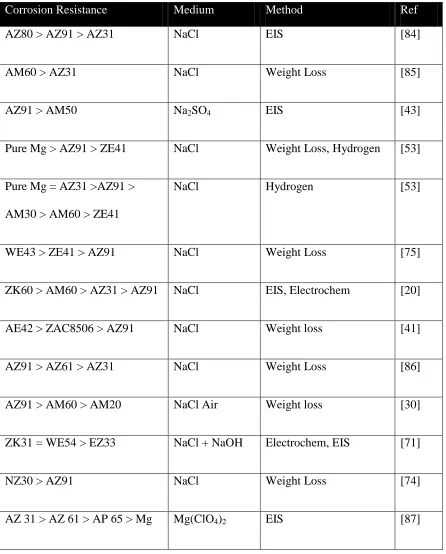
Table 1. 1 - List of common alloy elements and their effect in Mg alloy systems ... 8

Table 1. 2 - List of common Mg alloys and their applications ... 9

Table 1. 3 - The electrochemical series showing the standard reduction potentials for

elements relevant to this thesis [61] ... 29

Table 1. 4 - List of comparative corrosion rates of Mg alloys ... 34

Table 5. 1 - Quantitative XEDS data of the major elements from the corresponding

(24)

xxiii

Figure 1. 1 - a) Predicted fuel consumption by automotive fleet in Canada b) resulting

emission by-product production (ton x 105 CO2, NOx, CO. SO2 tons) ... 2

Figure 1. 2 - Canadian green house gas emissions by sector . ... 3

Figure 1. 3 - improvement in fuel economy (orange) and engine efficiency (red) from the

inception of fuel efficiency regulations to the present ... 5

Figure 1. 4 - the relationship between fuel economy and vehicle weight ... 6

Figure 1. 5 - Pourbaix diagram for the Al-water system at 25 °C and [Al3+] = 10-6 M .. 13

Figure 1. 6 - - Butler-Volmer relationship for a reversible metal dissolution/deposition

reaction. The solid line represents the measurable current and the dashed lines are the

partial currents for the two reactions ... 18

Figure 1. 7 - Butler-Volmer relationship for a metal dissolution/deposition reaction and

an oxidant/reductant reaction. When coupled, the anodic component of one reaction and

the cathodic component of the other have equal currents at ECORR ... 19

Figure 1. 8 - Current-potential relationships for the anodic and cathodic half reactions

plotted as Evans diagrams. The red markers indicate a system with an accelerated anodic

process... 21

Figure 1. 9 - Pourbaix diagram for the Mg-water system ... 23

Figure 1. 10 - Schematic of the accumulated corrosion product on Mg materials showing

an outer platelet-like layer of Mg(OH)2 and an inner layer of MgO ... 25

Figure 2. 1 - Schematic of a scanning electron microscope …….………56

Figure 2. 2 - Schematic showing the excitation volume caused by an incident electron

(25)

xxiv

Figure 2. 4 - Customized setup for CLSM analyses of corroded samples. ... 61

Figure 2. 5 - SEM BSE micrographs showing an AM50 Mg alloy surface in different

stages of sample preparation and the gradual revealing of the alloy microstructure at a)

1200 grit SiC, b) 2400 grit SiC c) 4000 grit SiC, d) 3-μm diamond paste and e) colloidal

silica polishing steps. ... 65

Figure 2. 6 - Experimental set up for intermittent immersion experiments. ... 65

Figure 2. 7- SEM images showing relocating of a selected AOI on a ZEK100 Mg alloy:

a) location of AOI relative to scratch, b) the selected AOI, c) the surface with the scratch

following a 24 h immersion in 0.16 wt% NaCl, d) the corroded AOI ... 67

Figure 2. 8 - SEM BSE micrographs of a AM60 Mg alloy following 48 h of immersion

in 1.6 wt% NaCl showing; a) the corrosion damage observed in the middle region of the

sample and b) identical corrosion damage located near the artificial scratch. ... 69

Figure 2. 9 – CLSM micrographs of a) a colloidal silica polished AM50 Mg alloy

displaying residual scratches marked with green arrows, b) following 96 h of immersion

in 1.6 wt% NaCl; the green arrows show the same residual scratches are still visible .... 69

Figure 2. 10 - 3D CLSM micrograph of an AZ31 Mg alloy surface exposed for 48 h in

0.16 wt% NaCl: a) with the accumulated corrosion product on the surface and b)

following removal of the corrosion product with chromium treatment ... 71

Figure 2. 11 - SEM micrographs of an AM50 sand cast sample a) after 12 h of

immersion in 1.6 wt % NaCl and removal of the corrosion product and b) after a 12 h

subsequent exposure of a location where major damage has occurred as a consequence of

(26)

xxv

experiment; θ indicates the phase angle between the two signals ... 73

Figure 2. 13 - Example of the estimation of Rp from a Nyquist EIS plot. Using the experimental data (red) the semicircle is extrapolated to the real axis (Z’) to find Rp .... 73

Figure 3. 1 - a) SEM backscatter image of a selected area of interest (AOI) on a sand cast

AM50 alloy and the corresponding EDX maps for b) Mg, c) Al, d) Mn ... 84

Figure 3. 2 - SEM and CLSM images of the AOI on an AM50 sample corroded through

successive wet-dry cycles following a) 0 h, b) 24 h, c) 48 h, d) 72 h and e) 96 h exposure.

The intermetallic marked with the arrow in a) is displayed in Figure 3.5. ... 85

Figure 3. 3- SEM micrograph of a sand cast corroded surface after 96 h continuous

exposure in 1.6 wt% NaCl ... 87

Figure 3. 4 - Progress of corrosion near a β-phase region following a) 24 h, b) 48 h, c) 72

h, and d) 96 h of immersion in 1.6 wt% NaCl ... 89

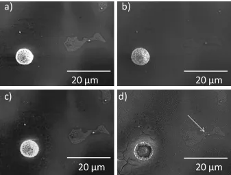
Figure 3. 5 - Progress of corrosion near an Al-Mn intermetallic from Figure 2a)

following a) 24 h, b) 48 h, c) 72 h, d) 96 h of immersion in 1.6 wt% NaCl. The white

arrow in d) shows a Al-Mn intermetallic with no corrosion product dome. ... 90

Figure 3. 6 - Identification of the location of α-grains on sand cast AM50 alloys using

EDX mapping. Grains were numbered for further analysis shown in Figure 3.8. ... 92

Figure 3. 7- a) CLSM image showing the location of a depth profile line scan in green

(bottom to top) and b) the corresponding changes in depth throughout the successive

(27)

xxvi

as a function of corrosion exposure time. ... 94

Figure 3. 9 - a) A FIB cross section of a β-phase region including the adjacent only

slightly corroded region after 96 h of corrosion: b) a TEM slide of the selected region; c)

O, Mg and Al EDX maps of the area marked in green; d) similar EDX maps of the red

area shown in b). ... 95

Figure 3. 10 - a) an AOI on a sand cast AM50 alloy prior to corrosion, which was

subsequently immersed for 24 h in 1.6 wt% NaCl: b) the AOI (red box) following the

immersion surrounded by a major corrosion event... 96

Figure 3. 11 - a) Montage image of a polished sand cast AM50 surface and images of the

same area following b) 2 h, c) 3h and d) 4h of immersion in 1.6 wt% NaCl. New damage

sites are marked with arrows... 98

Figure 3. 12 - Progression of areas which sustained major corrosion events: the corrosion

damage is observed to penetrate into the alloy but not to spread across the surface. ... 100

Figure 4. 1 - a) SEM image of a polished sand cast AM50 sample and the corresponding

EDX maps showing the distribution of b) Al, c) Mg and d) Mn throughout the area of

interest ... 112

Figure 4. 2 - a) SEM image of a polished graphite cast AM50 alloy and the

corresponding EDX maps showing the elemental distribution of b) Al, c) Mg and d) Mn

... 113

Figure 4. 3 - a) SEM image of a polished die cast AM50 sample and the corresponding

(28)

xxvii

die cast (red) AM50 alloys in 1.6 wt% NaCl at a scan rate of 0.5 mV/s after 20 min at

ECORR ... 116

Figure 4. 5 - Progression of ECORR of the polished sand cast (green), graphite cast (blue)

and die cast (red) AM50 alloys recorded in 1.6 wt% NaCl ... 116

Figure 4. 6 - Nyquist plots for the sand cast (green), graphite cast (blue) and die cast

(red) alloys recorded in 1.6 wt% NaCl after 10 h exposure... 117

Figure 4. 7 - a): SEM micrographs and CLSM images of the sand cast AM50 alloy after

a sequence of 24 h intermittent immersions in 1.6 wt% NaCl The red arrow identifies

domes of corrosion product appearing over sites of higher cathodic activity, b) SEM

micrographs and CLSM images of the graphite cast AM50 alloy after a sequence of 24 h

immersions in 1.6 wt% NaCl c) SEM micrographs and CLSM images of the die cast

AM50 alloy after a sequence of 24 h immersions in 1.6 wt% NaCl. The red arrows

indicate the location of a major corrosion event ... 119

Figure 4. 8 - SEM montage micrographs of the graphite cast AM50 after a) polishing, b)

2 h and c) 4 h intermittent immersions in 1.6 wt% NaCl. The red arrow in c) shows the

first major event to initiate ... 121

Figure 4. 9 - SEM montage micrographs of die cast AM50 after a) polishing, b) 2 h and

c) 4 h intermittent immersions in 1.6 wt% NaCl ... 121

Figure 4. 10 - Stereo micrographs of the a) sand, b) graphite and c) die cast AM50 alloys

following a 24 h immersion in 1.6 wt% NaCl. The white blotches on the sand and

graphite cast is the accumulation of corrosion product in the α-Mg regions while damage

(29)

xxviii

Figure 5. 1 - a) SEM micrograph of a polished AZ31 Mg alloy surface, b) SEM

micrograph of the Al-Mn intermetallic marked with the white arrow in (a), c) XEDS

spectra of the locations marked in (b), d) SEM micrograph of the domes of corrosion

product that appeared above the Al-Mn intermetallic particles marked with the red arrow

in (a) following 24 h immersion in 0.275 M NaCl ... 138

Figure 5. 2 - a) I) SEM backscatter micrograph of the a) Al-11Mn and b) Al-25 Mn

surface following polishing and the corresponding XEDS maps for II) Al, III) Si and IV)

Mn ... 140

Figure 5. 3 - Evolution of ECORR over a 12 h period of immersion in 0.275 M NaCl and

0.138 M MgCl2 for the Al-11Mn and Al-25Mn electrodes ... 142

Figure 5. 4 - PDP scans recorded on the Al-11Mn and Al-25Mn intermetallics in 0.275

M NaCl and 0.138 M MgCl2 from ECORR to -1.55 V at a scan rate of 1 mV/s ... 142

Figure 5. 5 - Potentiostatic current density vs. time profiles recorded on the Al-11Mn and

Al-25Mn electrodes at -1.55 V in 0.138 M MgCl2 and 0.275 M NaCl ... 143

Figure 5. 6 - optical micrographs of the Al-11Mn surface following a 20 h exposure to a)

0.275 M NaCl at ECORR, b) 0.138 M MgCl2 at ECORR , b) 0.275 M NaCl at -1.55 V, and c)

0.138 M MgCl2 at -1.55 V ... 144

Figure 5. 7 - a) SEM micrograph of the surface of the Al-11Mn electrode and b) the

corresponding XEDS spectra recorded after 20 h cathodic polarization at -1.55 V in 0.275

(30)

xxix

polarization at -1.55 V in 0.275 M NaCl. The oxide/base metal interface is marked with

the dashed line b) corresponding XEDS spectra for the locations indicated in (a) ... 147

Figure 5. 9 - a) SEM micrograph of the Al-11 Mn surface following cathodic

polarization for 20 h at -1.55 V in 0.138 M MgCl2, b) FIB cross section through the

surface layer with the red dotted line denoting the substrate/layer interface and c) XEDS

spectra recorded at the locations labelled in (b) ... 149

Figure 5. 10 - spectra identifying the phases present on the Al-11Mn electrodes after

cathodic polarization in (a) 0.275 M NaCl and (b) 0.138 M MgCl2 solution ... 150

Figure 6. 1 - a) BSE SEM micrographs of the ZEK100 surface. An intermetallic particle

is marked with the red arrow. The corresponding XEDS maps for b) Mg, c) Zn, d) Zr 166

Figure 6. 2 - a) SEM micrographs of the particle marked by the blue arrow in Figure 1a),

b) SEM micrograph of the particle marked with the red arrow in Figure 1a); and c) the

XEDS spot analysis of the corresponding areas marked in the SEM images ... 167

Figure 6. 3 - a) BSE SEM micrograph of the particle in Figure 2 (b) and the

corresponding XEDS maps for b) Mg, c) Nd and d) Zn ... 169

Figure 6. 4 – Potentiodynamic polarization scans recorded on a freshly polished ZEK100

sample at a scan rate of 0.167 mV/s following 1 h at ECORR in 1.6 wt% NaCl (black), 0.16

wt% NaCl (red) and 0.016 wt% NaCl ... 170

Figure 6. 5 - SE SEM micrographs of a ZEK100 sample following a) 24 h, and b) 48 h

(31)

xxx

solution. At 24 h the sample was removed for analysis, and then re-immersed again in a

new solution for an additional 24 h... 171

Figure 6. 7 - SEM micrographs of a selected area of interest on a ZEK100 sample: a)

and d) original polished surface : after 24 h of immersion (b) and e)) and 48 h of

immersion (c) and f)) in a 0.16 wt% NaCl solution. The red arrows are reference points

for two particles present in the AOI. ... 173

Figure 6. 8 - 2.5D CLSM micrographs of an AOI on the ZEK100 following a) 24 h and

b) 48 h immersion in a 0.16 wt% NaCl solution. A3D CLSM reconstruction of the AOI

following c) 48 h immersion in a 0.16 wt% NaCl solution and d) following a chrome

treatment to remove corrosion product ... 175

Figure 6. 9 – SE SEM micrographs of the ZEK100 sample surface after 48 h of

immersion in a 0.16 wt% NaCl solution showing a) the grain boundary regions filled with

corrosion product, b) following removal of the corrosion product, c) magnified image of

the corroded grain boundary ... 176

Figure 6. 10 - SE SEM micrograph of a) a corrosion product dome present on the

ZEK100 after 48 h corrosion in a 0.16wt% NaCl solution , and b) following removal of

the corrosion product showing the particles beneath the deposit: XEDS maps for c) Zn, d)

Nd, e) Zr, f) Fe ... 178

Figure 6. 11 - a) SEM image of two particles on the ZEK100 surface prior to corrosion

and the corresponding XEDS maps for b) Mg, c) Zr, d) Fe, e) Nd, f) Zn ... 179

Figure 6. 12 – a) SE SEM micrograph of the particles shown in Figure 11 following 6 h

(32)

xxxi

cathodic behaviour of the particle shown in the red box in (b): and the corresponding

XEDS maps of the site for d) Mg, e) Zr, f) Fe ... 180

Figure 6. 13 – The progress of corrosion of on a ZEK100 sample in NanoPureTM water

monitored by SEM showing an AOI after a) 24 h, b) 48 h, c) 96 h, d) 192 h: the progress

of corrosion around the particle at the bottom of the AOI after e) 24 h, f) 48 h, g) 96 h, h)

192 h of immersion ... 182

Figure 6. 14 – a) BSE SEM micrograph of the ZEK100 surface after 192 h of immersion

in water, b) BSE SEM micrograph of the area marked with the red box in (a) and the

corresponding XEDS maps for c) Zn, d) Nd, e) Zr and f) O, g) SE SEM micrograph of a

separate particle on the ZEK100 surface and its corresponding XEDS maps for h) Zr and

i) Fe ... 183

Figure 6. 15 – a) SE SEM micrograph of a corrosion product dome on the surface of the

ZEK100 sample after 192 h of immersion in NanoPure water: b) SE SEM micrograph of

a FIB cross at ¼ depth into the dome, c) FIB cross section at a location deeper into the

dome; d) SEM image revealing particle below corrosion product dome (marked with red

arrow), e) XEDS spectrum of the region marked with the red box in d) ... 185

Figure 6. 16 – Stereo micrographs comparing the bulk corrosion damage on the ZEK100

following a) 24 h of exposure in 0.16wt% NaCl and b) 192 h of exposure in NanoPureTM

water. The rolling direction (RD) of the samples is indicated with the arrow. ... 187

Figure 7. 1 - Coupling current-time profiles measured on a galvanic couple between

(33)

xxxii

shown in the inset... 200

Figure 7. 2 - Stereomicrographs showing the distribution of corrosion damage following

a 48 h immersion uncoupled in a1.6 wt% NaCl solution of a) sand cast , b) graphite cast ,

c) die cast AM50 alloys and following 48 h of galvanic coupling of the d) sand cast, e)

graphite cast and f) die cast AM50 alloys to pure Mg ... 202

Figure 7. 3 - Chronopotentiometric profiles recorded on the die cast AM5O in a 1.6 wt%

NaCI solution with applied cathodic current densities of -100 µA/cm2 (red), -1 µA/cm2

(green) and -0.1 µA/cm2 ( blue) ... 203

Figure 7. 4 - Stereomicrographs of the die cast AM50 alloy following 96 h of immersion

in a1.6 wt % NaCl solution: a) immersion with no electrochemical control, b) -100

µA/cm2 , c) -1 µA/cm2 and d) -0.1 µA/cm2 applied cathodic currents. ... 205

Figure 7. 5 - SEM micrographs of die cast AM 50 following 96 hr of immersion in a

1.6wt% NaCl solution: a) natural corrosion conditions; b) -1 μA/cm2 cathodic current

applied; c) -0.1 μA/cm2 cathodic current applied. ... 206

Figure 7. 6 - a) The progression of ECORR on a die cast AM50 alloy (blue) and potential

recorded with an applied current hold of -10 μA (red) in a 1.6 wt% NaCl solution. The

black arrow marks the location of a significant corrosion event. Stereomicrographs

showing the surface of die cast AM50 alloy after exposure at b) ECORR and c) -10μA

galvanostatic hold and d) magnified view of the corrosion track initiated ... 208

Figure 7. 7 - Chronopotentiometric plots recorded the die cast AM50 alloy in a 1.6 wt %

(34)

xxxiii

alloy : a) naturally corroding AM50 surface and b) a chronopotentiometrically controlled

surface ... 213

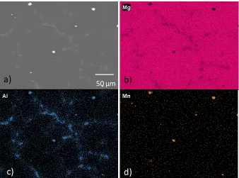
Figure 8. 1 - The microstructure of a sand cast AM50 Mg alloy displaying the common

microstructural features in a) SEM BSE image, and XEDS maps of (b) Mg, (c) Al, and

(d) Mn. A β-phase structure is marked in the images with a green arrow and an Al-Mn

intermetallic particle with a red arrow. ... 225

Figure 8. 2 - Evolution of ECORR measured on a sand cast AM50 Mg alloy in 3 mM

NaCl in water (black) and ethylene glycol (red) ... 227

Figure 8. 3 - A PDP scan measured on a sand cast AM50 Mg alloy in 3 mM NaCl in

ethylene glycol (red) and 3 mM NaCl in water ... 227

Figure 8. 4 - Progression of ECORR measured on a sand cast AM50 Mg alloy over a 48 h

exposure period in 3 mM NaCl + ethylene glycol with 2 mL additions of water made

after 3 h and 25 h. ... 229

Figure 8. 5 - Nyquist plots recorded on a sand cast AM50 Mg alloy after 20 h exposure

in 3 mM NaCl in water (black) and ethylene glycol (red). Inset: magnification of the high

frequency response in the aqueous solution ... 229

Figure 8. 6 - a) Progress of ECORR measured on a sand cast AM50 Mg alloy in 3 mM

NaCl + ethylene glycol. EIS measurements were made just before and after the addition

of 25 mL of water at ~ 2h: (b) Nyquist plots, and (c), (d) Bode plots recorded just before

(35)

xxxiv

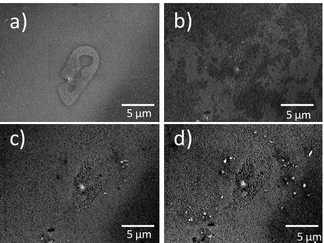
polished surface, b) following 72 h in 0.016 wt% NaCl in ethylene glycol, c) an Al-Mn

intermetallic marked in (a), d) the intermetallic following exposure having collected a

mass of corrosion product ... 233

Figure 8. 8 - Montage SEM map recorded on a sand cast AM50 Mg alloy. The red box

shows the location chosen for SECM measurements ... 234

Figure 8. 9 -area. The red arrow indicates two Al-Mn particles used to relocate this area

in images. (a) A cyclic voltammogram recorded on the Pt microelectrode in 1 mM

FcMeOH in ethylene glycol at 10 mV/s; (b) approach curves recorded at locations 1 and

2 (Figure 10 (a)) and the theoretically fitted approach curves ( and ) . I and II show

the calculated approach curves for a diffusion limited reaction and an insulating

unreactive surface, respectively. ... 236

Figure 8. 10 -(a) SECM map recorded on a sand cast AM50 Mg alloy in 1 mM FcMeOH + ethylene glycol using a Pt microelectrode polarized at 500 mV located 10 μm above

the surface and rastered across the surface at 10 µm/s: (b) an overlay of SEM and SECM

images of the same ... 236

Figure 8. 11 - (a) SEM BSE micrograph of the AOI on the sand cast AM50 Mg alloy

following the SECM measurement shown in Figure 10; and (b) SEM SE micrograph of

the AOI. Red arrows identify the same Al-Mn intermetallics in each micrographk ... 238

Fi gure 8. 12 - 3D CLSM micrographs of a) AM50 Mg alloy exposed for 24 h in

ethylene glycol and b) the AOI on the AM50 Mg alloy following the SECM

(36)

xxxv

(37)

Chapter One

Introduction 1.1 Introduction

Roads in Canada cover a distance of 1.4 million km, the equivalent of three and a

half trips to the moon [1]. As a result of this vast coverage the transportation sector

accounts for ~30 % of Canada’s energy demand, a level which is continuously growing

[2]. The petroleum demand of the transportation industry in Canada has grown from 79.6

million tons in 1990 to 103.1 million tons in 2011 [1]. Figure 1.1 (a) shows the expected

fuel consumption by the automotive contribution to the transportation sector up to

2035 [1]. An increase in gasoline consumption is expected up to 2025, after which it is

predicted to decrease to current levels by 2035. The emission by-products of petroleum

based fuels (CO2, CO, NOx) are harmful to the environment and detrimental to air quality

in urban areas. Figure 1.1 (b) shows the predicted annual Canadian production of these

by-products, and a direct trend between emission production and gasoline consumption

can be observed. By comparison to other sectors in Canada, the contribution to green

house gas emissions by the transportation sector is the largest and expected to grow,

Figure 1.2 [3].

In order to disturb the predicted trend, and lessen the environmental strain created

by the automotive industry two main approaches are being pursued: 1) improvements in

fuel efficiency and 2) powering the automotive fleet with alternative fuel sources.

Beginning in the mid-1970’s as a response to petroleum embargoes and increased

competition from foreign automotive manufacturers, both Canada and the United State

(38)

Figure 1. 1 - a) Predicted fuel consumption by automotive fleet in Canada b) resulting

emission by-product production (ton x 105 CO2, NOx, CO. SO2 tons) [1].

(39)

(40)

vehicle fleet has met these standards and out-performed the U.S. fleet annually [4]. The

implementation of these laws have resulted in decreased fuel consumption and improved

engine efficiency through improved vehicle, engine and drive train design, Figure 1.3 [4].

Alternative fueled, electric and hybrid vehicles have also been introduced to the market

with sales increasing annually. Restrictions in Li-ion battery technology, as well as

relatively low mileage per charge, have limited low cost and vast implementation of

electric vehicles in North America (~150 km) [5].

Specifically, General Motors (GM) addressed this environmental concern and is

set to reduce the CO2 footprint of individual vehicles by 20% by 2020 [6].

Complementing fuel and engine technology advancement to meet this goal is the

introduction of alternate structural materials in automobiles. A reduction in overall

weight improves the fuel efficiency of vehicles, as shown in Figure 1.4 [7]. GM has

acknowledged this benefit and will reduce the weight of vehicles by up to 15% by 2017

[6]. The most direct approach to lowering vehicle weight is replacement of steel and

other heavy fabrication materials in vehicles with lightweight materials such as Al alloys,

and the focus of this work, Mg alloys.

Auto-racing was the first vehicle sector to use lightweight Mg alloys in the

1920’s, and Volkswagen became the first commercial vehicle to include Mg alloys on its

Beetle in 1936 [8]. Today Mg alloys are included in the construction of a variety of

vehicle components such as front end carriers, brackets, seats, wheels, transfer cases and

instrument panels on a range of vehicles from the Ford F150 to the Chevrolet Corvette.

To meet the auto industry’s goal of weight reduction an increase in vehicle make up

(41)

Figure 1. 3 - improvement in fuel economy (orange) and engine efficiency

(42)

(43)

to investigate the microstructure influenced corrosion behaviour of lightweight Mg alloys

which are included or are candidates for inclusion in the vehicle fleet.

1.2 Magnesium and its Alloys

The primary advantage of Mg and Mg alloys is their light weight, with a density

of 1.74 g/cm3 [7]. This is 35 % lighter than Al (2.7 g/cm3) and nearly five times lighter

than steel (7.9 g/cm3) [8]. Pure Mg has poor physical properties and alloying is necessary

to tailor these properties to the specific requirements of a lightweight system.

Magnesium alloys are also ductile, easily castable and have good damping characteristics

[9]. These properties have led to its presence as a structural material in automobiles,

aircraft, aerospace, ballistics, electronics, bio-implants and armor [7, 9-10].

Mg is alloyed with many other elements to garner selected characteristics and the

common alloying elements, and the reason for their use, are shown in Table 1.1.

Varying the compositions of the additives can generate alloys fit for a desired

application. Much work has been done in the development of Mg alloys and new

compositions are constantly being developed to fill the lack of fundamental knowledge of

magnesium alloys [9]. Some recent developments have seen the introduction of

Mg-Zn-Sm [16], Mg-As [17], Mg-Li [18], Mg-Sr [19], Mg-Gd [20] in the past year. These

(44)

Table 1. 1 - List of common alloy elements and their effect in Mg alloy systems

Element Alloy Designation Properties Ref

Ag Q Improve elevated temperature

properties and creep when present with rare earths

[11]

Al A Improve castability, precipitation

hardeners produced, corrosion protection

[11], [12]

Ca X Grain refinement, improves creep

resistance, improve high temperature properties

[11], [13], [14]

Rare Earths (Ce, La, Nd)

E Improve creep resistance, castability, grain refining, age hardening

[13], [15]

Si S Improves creep resistance [13]

Sr J Improve creep resistance [14]

Mn M Purification [12]

Y W Improve tensile properties, grain

refining

[13]

Zn Z Ductility and castability [13]

(45)

Table 1. 2 - List of common Mg alloys and their applications

Name Composition

(Balance Mg, wt%)

Example Uses Ref

AZ31 3% Al-1% Zn-0.20%Mn Aircraft fuselage, cell phones, laptops

[7], [20]

AZ91 9% Al- 0.7 % Zn, 0.13 % Mn

Door mirror brackets, valve and cam covers, die casting

[9], [20]

AM50 5% Al- 0.13 % Mn trace Si Steering wheel arm, seats [9]

AM60 6% Al- 0.13 % Mn Car seat frames, steering wheel, inlet manifolds

[9][20]

ZE41 4% Zn – 1 % Nd Ballistics, aircraft parts [9]

QE22 2% Ag – 2% Nd Aerospace [21]

ZK 60 6% Zn - <1 % Zr Military components, tent poles, sports equipment

[9]

WE 43 4.3 % Y – 3 % RE – 0.4 % Zr

Helicopter transmission, race car

[22], [23], [24]

(46)

One of the factors (along with cost and formability) standing in the way of

extended application of Mg alloys is their poor corrosion resistance. Overcoming this

deficiency begins with fully understanding the processes influencing the corrosion of Mg

and its alloys.

1.3 Aqueous Corrosion

1.3.1 Thermodynamics of Corrosion

In the corrosion process of a material an interfacial reaction occurs between the

material and its environment, in which the material is oxidized and an environmental

species (H2O, O2) is reduced. The two processes form an electrochemical redox couple

and, as an example: the corrosion of Mg materials in aqueous environments involves the

coupling of two reactions [25]:

Anodic: Mg  Mg2+

+ 2 e- (1.1)

Cathodic: 2 H2O+ 2 e-  H2 + 2 OH- (1.2)

The driving force for the corrosion process is the difference in equilibrium

potentials for the two coupled half reactions. The tendency for the reaction to proceed is

given by the molar Gibbs free energy change (ΔGrxn):

(1.3)

Where µp and µr are the product and reactant chemical potentials and νp and νr are the

(47)

(1.4)

in (1.4) R is the universal gas constant, 8.314 J K-1mol-1, T is the temperature, µ° is the

standard chemical potential of the species and a is the activity of the species. The Gibbs

free energy of an electrochemical reaction at equilibrium can be defined as:

(1.5)

where n is the number of moles of electrons exchanged in the reaction, F is Faraday’s

constant (96485 C∙mol-1) and ΔE is the potential difference between the electrodes

carrying the anodic and cathodic reactions (ΔE = Ered – Eox). Combining the three

equations, 1.3, 1.4, and 1.5 yields the equilibrium potential (Ee) for a half reaction

expressed by the Nernst equation. For dissolution of a metal species the equilibrium

potential is defined as:

M(s)  Mn+ + n e- 1.6

1.7

and for its coupled cathodic process, the equilibrium potential is:

Ox + n e-  Red 1.8

1.9

where E° is the standard potential for the half reaction and a is the activity of the species.

The common way to display the Nernst equation for chemical and electrochemical

reactions of a material in aqueous environments is on a plot of potential vs. pH, known as

(48)

The equilibrium between Al and water will be used as an example since the

behaviour of Al is essential to portions of this work. The Al metal dissolution reaction is

given by the reduction reaction:

Al3+(aq) + 3 e-  Al(s) E°= -1.66 V (vs SHE) (1.10)

The Nernst equation for the reaction is:

(1.11)

Substituting in the known values gives (converting ln to log)

(1.12)

For a given temperature and Al3+ concentration, is constant and independent

of pH and will show up as a horizontal line in the Pourbaix diagram. The Pourbaix

diagram of Al is shown in Figure 1.5 with E displayed vs. the saturated calomel electrode

(-0.242 V vs. SHE) at [Al3+] = 10-6 M. The transition between Al and Al3+ is denoted by

the red line in Figure 1.5. At the conditions on the red line Al and Al 3+ will be in

equilibrium with one another while at potentials above this line, the Al metal is not stable

and will dissolve as Al3+, and the Al will continue to dissolve until a new equilibrium is

established in the system. At potentials below this line the Al exists as metallic Al and is

(49)

a)

b)

Figure 1. 5 - Pourbaix diagram for the Al-water system at 25 °C and

(50)

Metal dissolution reactions are not limited to solely electrochemical reactions and

can involve water, protons, oxygen and other species. In this system, Al can react with

water to form Al2O3 in the reaction:

Al2O3(s) + 6 H+(aq) + 6 e-  2 Al(s) + 3 H2O(l) Eo = -1.55 V (vs SHE) (1.13)

for which the Nernst equation is,

(1.14)

and can be rearranged to:

(1.15)

Now the equilibrium potential of this reaction is dependent on pH due to the involvement

of protons, and will show up as a straight line with a slope of -0.059, marked in green in

Figure 1.5. Above this line, Al2O3 is the stable species, while below it, metallic Al is

stable. This equilibrium line between Al and Al2O3 theoretically extends into the stability

region of Al3+ defined previously. Al3+ and Al2O3 can convert between one another via

the following reaction:

2 Al3+(aq) + 3 H2O(l)  Al2O3(s) + 6 H+(aq) (1.16)

This equilibrium reaction is a chemical reaction, and is independent of potential and

depends only on the solubility product of the equilibrium, Ksp.

(51)

In Figure 1.5, a [Al3+] = 10-6 M was used to construct the Pourbaix diagram and

substitution of this value into the Ksp equation reveals this equilibrium is established at

pH = 3.9. Therefore a vertical line, the blue line in Figure 1.5, represents the pH at which

Al3+ and Al2O3 are in equilibrium with one another. The lines for the other reactions

involving Al, Al  AlO2- and Al2O3  AlO2- are calculated in a similar fashion.

There are two more lines of interest in the Pourbaix diagram, shown as orange

dashes labelled (a) and (b) in Figure 1.5. These lines represent the oxidative and

reductive decomposition of water in the following two reactions:

2 H2O + 2 e-  H2 + 2 OH- (a) (1.18)

2 H2O  O2 + 4 H+ + 4 e- (b) (1.19)

The equilibrium potentials for these reactions are also defined by the Nernst

equation, are pH dependent and appear as lines with slopes of -0.059. In the region

between the two lines water is stable. However, if the reacting surface is polarized to a

potential below (line (a)) or above (line (b)) the line, the water reaction can be the

coupled reaction to the metal species reaction. For example, the equilibrium line for

Al3+/Al is at a potential below the water equilibrium line for water reduction up to pH 4.

Due to this scenario, Al is thermodynamically unstable in H2O at pH <4 and will oxidize

to Al3+ by coupling to the reduction of water. Between pH 4 and 9, Al will form a solid

Al2O3 that could protect the metal from corrosion. This oxide will grow when Al

oxidation is coupled with water reduction. Above pH 9, Al can corrode once again to

AlO2- in water. Pourbaix diagrams are highly informative for the identification of

possible species existing in a corrosion system, however care must be taken in

(52)

layer determine the extent of its protection to the base metal. The Pourbaix diagram also

lacks kinetic information about the reacting system, which will be discussed in the next

section.

1.3.2 Kinetics of Corrosion

When anodic and cathodic half reactions are coupled in a corrosion process they

form a short circuited galvanic cell. The positive current from the anodic half reaction(s)

(metal dissolution) is (are) equal and opposite in sign to the cathodic current from the

reduction of the oxidant(s). This current is carried via electrons in the metal and by ions

in solution. The resulting corrosion current, ICORR, is defined as:

ICORR = Ianodic = | Icathodic | (1.20)

If ICORR is known, Faraday’s law can be applied to calculate the amount of

material corroded:

(1.21)

where n is mol of electrons passed, F is Faraday’s constant (96485 C∙mol-1

), m is the

mass of corroded material (g), M is the molecular weight of the material (g∙mol-1

) and t is

the exposure time (s). However, the ICORR is not readily measurable with an ammeter as

the current flowing at the corroding surface is short circuited. Electrochemical analyses

can be employed to determine ICORR and ECORR information about the corroding system.

Focusing on a reversible metal dissolution/deposition reaction, M  Mn+

+ n e-, the

Butler-Volmer equation, equation 1.22, shows the current-potential relationship for the

(53)

(1.22)

where α is the transfer coefficient, η is the overpotential for the half reactions (a measure

of how far away from the equilibrium potential, Ee, the reaction is), Io is the exchange

current. Figure 1.6 graphically demonstrates the Butler-Volmer relationship for this

reversible process. The solid line is the measureable current while the dashed lines are

the partial currents for the two half reactions. At sufficiently large overpotentials (η = E

– Ee) one of the half reactions dominates and the measured current becomes equal to IA or

IC. However, near Ee, both half reactions are occurring and the measured current is the

sum, IA + (-IC).

For a sufficiently high anodic overpotential, the cathodic component of the

Butler-Volmer equation (far right term in equation 1.22) becomes negligible and the

Butler-Volmer equation condenses to:

(1.23)

which can be written logarithmically as,

Log Ia = log Io + 2.303

η (1.24)

A plot of log Ia vs η would yield a straight line with an intercept Io and a slope given by,

(54)

Reduction:

M

n+

_{+ n e}

-



_M

Oxidation:

M



M

n+

_{+ n e}

-I

o

E

e

η

Current

Potential

Figure 1. 6 - - Butler-Volmer relationship for a reversible metal dissolution/deposition

reaction. The solid line represents the measurable current and the dashed lines are the

(55)

E_e- cathodic

E_e- anodic

E_CORR

I_c

I_a

Po

ten

ti

al

Current Anodic

Cathodic

Oxidation:

MMn+_{+ n e}

-Reduction:

Mn+_{+ n e}-__M

Reduction:

Ox + n e-__Red

Oxidation:

RedOx + n e

-Figure 1. 7 - Butler-Volmer relationship for a metal dissolution/deposition reaction and an

oxidant/reductant reaction. When coupled, the anodic component of one reaction and the

(56)

This term is deemed the Tafel coefficient, β. The same procedure can be carried out at

high cathodic overpotentials.

For a corrosion reaction the anodic half of one reaction (e.g., the metal dissolution

reaction) couples with the cathodic half of another (the oxidant reduction) reaction. If the

equilibrium potentials of the two reactions are sufficiently separated then these reactions

will be irreversible and only one of the two exponential terms in the respective

Butler-Volmer equations will be required. A Butler-Butler-Volmer-like equation can be written for the

corrosion reaction,

(1.26)

where αa and αc are the anodic and cathodic half reaction transfer coefficients and ηa and

ηc are the anodic and cathodic half reactions. Figure 1.7 shows the coupling of two half

reactions and their Butler-Volmer relationship. The potential established by the coupled

reactions under open circuit conditions is the corrosion potential (ECORR). At this

potential both the anodic current (Ia) from the metal dissolution reaction and cathodic

current (Ic) from the reduction of the oxidant are equal to one another. Both of the half

reactions are polarized away from their respective Ee until equal currents are established.

The overpotentials (η) in equation 1.26 are given by the difference between Ee and ECORR

for the two half reactions involved.

The influence of the kinetics of the two half reactions on ECORR is best shown in

an Evans diagram of potential vs. log I, Figure 1.8. The ECORR of a system, and the

resulting ICORR, can be shifted as the half reaction kinetics are altered. In a corroding

(57)

Po

ten

ti

al

Log Current

ECORR

Oxidation:

MMn+_{+ n e}

-Reduction:

Ox + n e-_Red

Ee- cathodic

E_e- anodic

I_CORR

ECORR

I_CORR

Figure 1. 8 - Current-potential relationships for the anodic and cathodic half reactions

plotted as Evans diagrams. The red markers indicate a system with an accelerated anodic

(58)

anodic reaction kinetics are accelerated (red line) in which case higher currents would be

observed at lower potential, ECORR is lowered to a less positive value, and ICORR would

increase. A commonly applied trend is a decrease in ECORR corresponds to an increase in

ICORR.

1.4 Corrosion of Magnesium and its Alloys

1.4.1 Corrosion of Mg

The corrosion of Mg appears a simple process, but is heavily debated. The

simplicity of the general corrosion behaviour of Mg is seen in the Mg-H2O Pourbaix

diagram, Figure 1.9 [28]. Mg can only exist in its metallic state at very low potentials

( < -2.4 V vs. SHE), and will be oxidized to Mg2+ above this potential. Mg(OH)2 is the

thermodynamically stable corrosion product above pH 8, and should be controlled by its

Ksp (5.6 x 10-12). This is an unusually straightforward system compared with many other

metal-H2O systems [26]. Two species are listed in the Pourbaix diagram whose existence

is debatable (denoted with a ? in Figure 1.9): univalent Mg+ and MgOx. Their importance

will be discussed in subsequent sections.

With the equilibrium potential for Mg oxidation positioned well below the water

stability region in the Pourbaix diagram (line (a)), the reduction of water is a readily

available cathodic reaction to drive Mg. The corrosion half reactions are commonly

reported as [25]:

Anode : Mg(s)  Mg2+ + 2 e- (1.27)

(59)

(60)

which combine to yield the overall reaction of [29]:

Mg(s) + 2 H2O(l)  Mg2+(aq) + 2 OH-(aq) + H2(g) (1.29)

Since the difference in Ee between the two half reactions is extremely large the corrosion

kinetics are fast and the generation of OH- will increase the interfacial pH eventually

leading to the deposition of Mg(OH)2,

Mg2+(aq) + 2 OH-(aq)  Mg(OH)2(s) (1.30)

However, since H2 is also formed, gas evolution from the Mg surface prevents the

depositing Mg(OH)2 from forming a compact layer, and the resulting deposited corrosion

product has a broken, porous, platelet-like structure, which does not passivate the Mg

surface [30-32].

1.4.2 The Corroding Surface of Mg and its Alloys

The corrosion products formed on Mg and its alloys have been reported to be an

outer layer of Mg(OH)2 and an inner compact layer of MgO [30-35], and this structure is

shown schematically in Figure 1.10 [36]. It has been suggested that the MgO is a

“protective” air form film on the material surface, but this has not been unequivocally

demonstrated [37]. On alloy surfaces, a mixed Mg/Al oxide has been identified [38] and

shown to be present in the outermost regions of the corrosion product layer [31]. At the

base of this layer it has been reported that an Al layer is formed [33, 36, 39] and is linked

to the corrosion resistance. In Zn-containing Mg alloys, a accumulated Zn layer has also

been reported to form at the corrosion product/alloy interface which has also been

(61)

Figure 1. 10 - Schematic of the accumulated corrosion product on Mg materials

(62)

Mg alloys does not occur homogeneously with areas covered by substantial deposits, and

domes of corrosion product developing as corrosion progresses [28, 40].

This accumulated corrosion product layer does not passivate the alloy under non

alkaline conditions (< pH 13) [41] due to its porous nature [42]. However, the

development of the corrosion product layer has been linked to decreased corrosion rates

[33, 43] most likely a consequence of reduced cathodic kinetics [40, 44].

1.4.3 Magnesium’s Great White Buffalo: The Negative Difference Effect and Mg+

In the Pourbaix diagram for the Mg-H2O system, unipositive Mg+ is commonly

included although its existence is commonly debated in the literature. It is claimed that

the existence of Mg+ as an intermediate in Mg corrosion can be attributed to the peculiar

behaviour of Mg under anodic polarization. It would normally be expected that when Mg

is polarized to a potential anodic to ECORR by the imposition of an applied current, two

effects would be expected: 1) the anodic half reaction rate should be increased (oxidation

of Mg to Mg2+), and 2) the cathodic half reaction rate should be decreased (reduction of

H2O water to H2). However, the measured amount of H2(g) evolved when an anodic

current is applied is higher than the amount evolved at ECORR: this has been termed the

negative difference effect (NDE) [45]. The widely reported explanation of this effect

involves the participation of unipositive Mg species (Mg+) in the corrosion process [12,

37, 42-43, 45-49]. In electrochemical reactions involving more than one electron, it is

rare that electron transfer occurs in a single step [25], and it has been suggested that Mg

is initially oxidized to Mg+, which subsequently undergoes a chemical reaction to evolve

(63)

Mg  Mg+

+ e- (1.29)

Mg+ + H2O  Mg2+ + OH- + ½ H2 (1.30)

The proposed explanation for this effect is that the anodic current applied

increases the generation of Mg+ which can either be further oxidized to Mg2+or evolve

more H2 by reaction (1.32), despite the applied anodic polarization. However, the

presence of Mg+ as a surface species has never been spectroscopically identified or

analytically isolated [25]. The existence of Mg+ is based on the observation that

permanganate is reduced on an anodically polarized Mg alloy surface in Na2SO4, and the

assumption that the only available reducing agent would be Mg+ [50]. Recently, it has

been shown that at the negative potentials around the ECORR of Mg (~ -1.6 V vs SCE),

SO42- is converted to SO2, making this the reducing agent for permanganate rather than

Mg+ [51].

Recent investigations have called the unipositive Mg+ explanation into question

[25, 52-58], on the basis that the amount of evolved hydrogen does directly correlate to

the amount of dissolved Mg (as Mg2+) based on measured corrosion rates via mass loss,

hydrogen collection and electrochemical measurements. No chemical step appears to be

involved since the Faradaic ratio between the amount of Mg dissolved and the integrated

applied current is nearly equal to one [58]. It has been suggested that the increased H2

evolved under anodic control is a result of an increased cathodic capability of the Mg

electrode as it is oxidized [57,59] and possibly through enrichment of elements which are

cathodic to Mg [60].

It is reasonable to presume that the sites cathodically active on a corroding Mg