Abstract. Density of supercooled water at elevated pressure is interesting because of the strong anomalies which can be explained by existence of a liquid-liquid critical point in the region of supercooled water. In order to provide accurate data for density at these conditions a procedure was developed to calibrate the course of the inner cross section of a capillary along its length. Further, the image analysis for the sub-pixel evaluation of meniscus postion is described.
1 Introduction
A new experimental setup for measurement of density in supercooled liquids has been built at the Institute of Ther-momechanics in Prague. The apparatus is a significant con-tribution to extensive effort to determine thermodynamic properties of supercooled water, for following previous ex-perimental studies of density [1], [2] and [3]. The prop-erties of supercooled water are important from practical point (meteorology, climate models, cryobiology) and the-oretical point of view as well (as an experimental evidence of the existence of second critical point [4]). The measure-ment is based on the thermal expansion under specified pressure and temperature (for a detailed description see [7]). To achieve deep supercooling, the volume of liquid should be as small as possible. Therefore, synthetic fused silica capillary was applied.
The capillary manufacturer Macherey-Nagel GmbH & Co. KG presents a capillary inner diameter of 0.320 mm, with claimed uncertainty+/- 4.9μm. However, for a pre-cise density measurement in our apparatus the develop-ment of the cross-section along the capillary length is es-sential. Present paper describes an apparatus and data pro-cessing necessary to measure the capillaries cross-section area of the capillaries.
2 Measurement method
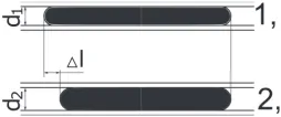
A drop of mercury is inserted into a capillary. Due to its high surface tension the mercury remains in one slug over the experiment. At a specific position the mercury occupies a given volume and so a specified length, like in figure 4. If the slug is moved to another position the length changes due to the diameter change. To use effectively such a method it is assumed, that the diameter change over a short length is small. A similar principle was used already in the 19th century for calibration of mercury thermometers, like presents Maxwell in his book [5].
a e-mail:[email protected] b e-mail:
[email protected] c e-mail:
[email protected] d e-mail:
Figure 1.Comparison of two diameters with the same mercury slug.
3 Experimental setup
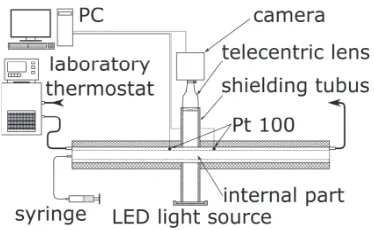
A special setup shown in figure 2, was developed to imple-ment the calibration method.
The capillary is fixed to a groove in a specially pre-pared Plexiglas ruler shown in figure 3. The groove is made such that the upper surface of the capillary touches the plane which is defined by the upper side of the ruler. Above the groove tiny holes were located, which were used as a length coordinate. The ruler is inserted in to a brass block with an observation window. The observation window in the block is equipped with a fixed precise glass scale for determination of the mercury slug length. To ensure a con-stant temperature for the measurement, the brass block is equipped with tempering channels and it is insulated from the outside. The tempering channels were attached to a lab-oratory thermostat. To monitor the temperature at the ob-servation region two Pt100 TRD elements were inserted and the data were continuously recorded along the mea-surement.
A gas tight Hamilton syringe is connected via a silicon hose at one end to the capillary to allow movements of the mercury slug to a required position.
For length measurements of the mercury slug inside the capillary a monochromatic digital laboratory camera with an attached high resolution telecentric lens with minimized optical aberration effect is used. The pictures were saved directly to a computer and later evaluated.
The measurement proceeds in the following way. The capillary is filled with a mercury drop and the ruler is in-serted in the brass block so that, the desired capillary zone is visible in the camera. Commonly is the ruler position set so, that in the middle of the picture is visible the rulers position hole. For the first time of a new measured set is the camera focused on the capillary and scale, they both
Figure 2.Experimental setup overview.
Figure 3.Detail view on the internal part.
located within the focused deep of field. The laboratory thermostat is turned on and set on 25◦C. The temperature was stable to 0.05◦C.
The mercury slug is pushed by the syringe to the re-quired position in the camera view. If the temperature is stabilized, the required picture could be taken. In figure 4 is shown a typical image.
After images at all ruler coordinate points were taken, images were evaluated.
4 Image analysis
Figure 4 shows an image with all demanded elements nec-essary for the complete data analysis. A ruler coordinate point with its number, scale and capillary with the mercury slug had to be present. The camera sensors horizontal and vertical lines had to be aligned with the capillary and scale. The maximal tolerated deviation for a horizontal line is up to three pixels in vertical direction over the whole image. That had a negligible impact on the results (less than 2μm on the whole range).
The evaluation is mostly automatized and could be di-vided in few main parts. Determination of the picture res-olution, finding the position of the ruler coordinate point, finding the capillary and determine the menisci.
It’s assumed, that the image set taken at measurements is processed at once.
To understand the following sections it is appropriate to know how matlab handles common images. A monochro-matic 8 bit image is a common matrix. Its size corresponds to the resolution and every element represents a light level value. The light level is an unsigned 8 bit integer variable. The value of zero could be interpreted as totally black. Then small graduation of light intensity moves up to 255 which mean totally white. It should be mentioned, that matlab also support only two state eq. black and white pic-tures (0 is black, 1 is light), colored picpic-tures (which were
Figure 4.Image for data analysis.
used for result visualization for the user who checks the data) and 16 bit pictures (if the source had the capability to capture images with finer light level resolution, ie. up to 65 636 levels).
4.1 Pixel size
For every image is the pixel size computed, to ensure every time correct values.
For a fast and a robust evaluation the user had to draw a rectangle over the whole scale for the first image. The se-lection is applicable for the whole set, because now visible movement of the scale is present for the whole time.
Now the long horizontal line is searched. The light in-tensity values across every horizontal line in the user se-lected rectangle is summed and stored with its vertical po-sition. The line with the lowest sum of light intensities is the searched.
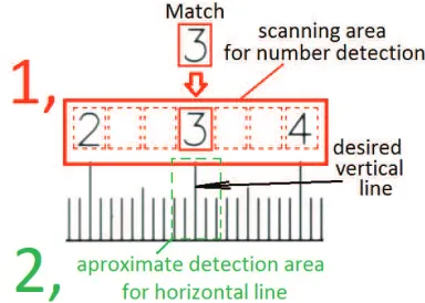
In the next step the position of defined scale numbers had to be found. That’s necessary to find the approximate position of desired vertical lines (the longer vertical lines right beneath the numbers). Lin’s concordance correlation coefficient [6] is used to determine the right number. Also Pearson’s correlation coefficient could be used. The results for all tested methods were the same.
For a given set of images were needed reference im-ages. They had to be created for the first time of an eval-uation. If the same numbers were present in another set of images, the reference images don’t have to be recreated (for all tested sets worked well, the first taken reference images).
Now every number had a reference image.
Figure 5.Detection of scale number and the position of the de-sired vertical line.
marked as unfindable. Partially is this step shown as one in figure 5.
In the next step, the longer vertical line below the scale number is searched. In a defined area, like it is shown in step two in figure 5, the minimum median value of the image matrix columns is searched. The median is used to discard potential dirty spots or scratches in the searching area. The column with the lowest median value represents the searched line.
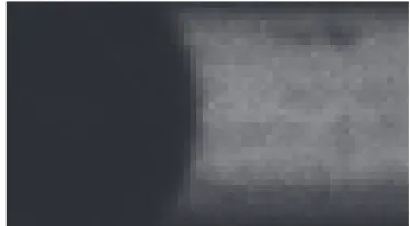
The now defined position for the given line is rough, because the criterion is not sufficiently confident. The scale lines in reality are not only one pixel width, align exactly with the camera points and were not totally dark. Com-monly the lines were little transparent and had a width up to five pixels with a smooth transition boarder, like could be seen in figure 6. To identify the center of the line an area, little wider than the line and only 50 point high is taken for further evaluation. Now were taken column median values of the light intensity from that part. All points which fall into a light range between 0 to 85% of the line intensity range were used for a polynomial fit of second order. The inflection point is the searched middle of the line with and sub pixel accuracy. For the smoothness were used number with an order of 0.01 pixel, but in real it is slightly lower. The comparison for a line, which has it center approximate in the middle of pixel column is to see in figure 6. The bro-ken line represents the computed median values, where the continuous line shows the fitted curve. Another interesting thing is the transparency of the line, which is good to see. Because the minimum for the lines falls only to a
Another interesting thing which is to see from the chart is the permeability of the scale line, because the lowest value evaluated by the median is not something about zero, but 110. That is about a half in the intensity range.
Not every time looks the line like in figure 9, but some-times the signal could look like in figure 11. The light value, between two points is similar, with a higher ten-dency to the point on the right. So with the interpolation, the setting point is selected about 1/4 of the distance be-tween the point from the right point, which approximately corresponds to the expected value.
The mentioned workflow is repeated totally for six times, common for numbers 2, 3, 4, 16, 17, and 18, so if one line value is bad detected it would be out selected by the last task. Now all pairs of numbers which had a farther diff er-ence than ten were evaluated to get the number of pixels per mm, see equation 1. WhereΔliis the difference of two
Figure 6.Enlarged detail of a line.
Figure 7.Median comlumn values of light intensity of a line like in figure 6.
Figure 8.Median comlumn values of light intensity of a line with a unclearer center postion.
numbers above the vertical scale lines,Δxiis the horizontal number of pixels between the two vertical lines (due to the mentioned method that number don’t have to be integers) andRi is the resolution or number of pixels for 1 mm in the end the value ofR−1is the searched size in mm for one pixel.
Ri= ΔΔxi li.
(1)
4.2 Ruler coordinate point
Figure 9.Median of light intensity for a cut of horizontal lines on the left edge.
the required circle. If no circle is founded, the value of the sensitivity is slightly increased and the function is started again. That process is repeated until at least one circle is found. If the sensitivity value reaches 1, the loop is stopped and the circle position is set to ”not present”. If more than one circles are detected, the user had to select the right one in the check part implemented in the post processing part.
4.3 The mercury slug
For the first picture in the set, a rectangle area of the capil-lary with the mercury slug had to be drawn. Now a vertical search for the capillary is started. Figure 9 shows median values of horizontal lines inside the selected area. The zone of the capillary had a typical progress. The light intensity decrease from the maximum, rise a little (the area where the light shine trough), decrease and rise to the maximum. The two minimums had every time a minimal size of 10 pixels. A similar progress could be expected for all pic-tures.
A cycle in the detection function was written, to get the upper edge of the capillary. The upper edge is defined by detection of an interval where light intensity decrease for the first time to a value below 20% of the given range for at least 10 pixels. For the bottom line is used the same workflow, but the cycle goes from bellow. That rough but fast detection is used to shorten the investigation area for the next step.
To find the left and right meniscus relative exactly, the correlation coefficient of Lin was used. Pearson’s coeffi -cient was tested too, with the same results. For that pur-poses existing two reference images, one of every menis-cus. The scanning area is defined by the detected capillary boarders and the systematics is the same like mentioned in section 4.1. The approach again worked well for all tested images and eliminates the problem with sometimes occur-ring spots of dirt and scratches.
Finally the meniscus top had to be found. The process will be explained on figure 10.
Before the process will be explained a detailed investi-gation on the transition area in the image had to be done. Figure 11 shows a chart of horizontal line light intensity progress with the horizontal coordinate. The meniscus lo-cation could be determined, but not easily and exactly enough. Now the transition is about 6 to 7 pixels. Figure 12 come handy here. It shows light intensities along vertical lines
Figure 10.The founded meniscus.
Figure 11.Horizontal line light intensities for right meniscus.
Figure 12.Vertical line light intensities for right meniscus.
from the observed areas. Here is nice to see the slow rise of the intensities. A roughly shape of the meniscus could be seen. Another thing that could be observed in the two pic-ture is the maximal light intensities at the horizontal lines, where the inner diameter of the capillary ends, due the cap-illary curvature.
A definition had to be determined to get the accurate position for the meniscus boarder. To use also the area with the lower light values, it was chosen to define the boarder location where the intensity of the line becomes exactly the half value of the line range in the observed area. So a threshold value was computed for every horizontal line. Those values were used to transform the image to a two state matrix. In the first stage was from the two state ma-trix detected the position where the threshold value was exceeded.
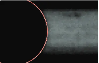
Figure 13.Meniscus with osculation circle.
threshold value was exceeded. That criterion is acceptable, because the system and compared data remain the same over the whole evaluation of the one set.
The received position data of the meniscus were taken for a polynomial fit of the second order. And the curve top is decided as the meniscus top. That is also done be-cause sometimes some spots with lover light intensity in the meniscus area occur which could else totally devalue the data and result in misleading values. To detect the data health an osculation circle is constructed at the curve top. If the radius of that circle is in and range of 0.75 to 1.25 to the capillary range, the data were considered as satisfying, else they were discarded.
In figure 13 is shown the resulted osculation circle of the meniscus in figure 10
4.4 Data health inspection
Despite all protection mechanisms a small possibility of wrong detection remains. To ensure that only correct data will be used for the final evaluation, the user had to do a visual check of the whole set.
For that purpose is written a script. It shows the orig-inal source image which had overlaid the elements which should be checked. Figure 14 shows the whole inspection picture, for ruler coordinate point 0 (the only one without a number). There is nice to see the fit of the ruler coordinate point. The osculation circle of the left meniscus shows ok too. The right meniscus osculation curve is too huge, so the image results were not usable.
Although the fault was known before, the image was totally preceded and shown to the user. Based on the crite-ria, the image in figure 14 is automatic discarded due the inspection. Multiple detected ruler coordinate points could be corrected here. Or image values which possible fooled the checking mechanisms could be manually out sorted. For that purposes a more detailed view is used due the check, like in figure 13. Necessary accompanying infor-mation like file name, coordinate point number etc. where shown in the console.
5 Results
The dependence of the mercury slug center positions to its length, represent indirect the searched parameter. A repre-sentative result is shown in 15. Because some points were measured two times and the values don’t match exactly, some of the data had a visible small jump. Finally it is to
Figure 14.Image for user inspection.
Figure 15.Vertical line light intensities for right meniscus.
Figure 16.Relative variation of the cross section area.
see that the mercury slug is longer in the first part of the capillary and decrease in the second half.
The cross section area is the desired parameter, but it could be only computed as a relative ratio, because the vol-ume of the mercury slug is unknown. The ratio of the cross section A A
reference is direct related to the length ratio
Lreference
L , like is mentioned in equation 2. The index reference sym-bols represent a chosen reference length or diameter. The reference length is determined as the median value of the whole measured set.
In figure 16 is presented the relative percentage change of the area to the reference area. The progress of the cross section area is inverted to the length of the mercury slug like it was expected.
A Areference =
Lreference
L . (2)
It was expected that the capillaries had not a totally equal diameter eq. cross section over the whole length. The experiment shows it pretty good in figure 16. The deviation for the measured capillary goes from -2 to 6 % of the cross section.
evaluation are proper for cross-section determination along the capillary tube.
Acknowledgements
The authors gratefully acknowledge a support by grant No. GAP101/11/1593 of the of the Czech Science Foundation. Participation in IAPWS activities was supported by grant No. LA09011 of the Ministry of Education, Youth and Sport of the Czech Republic.
The project has been also supported by internal grant 902129 from the Institute of Thermomechanics AS CR, v.v.i, and the institutional support RVO:61388998.
References
1. T. Sotani, J. Arabas, H. Kubota, M. Kijima, High Temp. High Pressures32(2000)
2. B. Guignon, C. Aparicio, P. D. San, J. Chem. Eng. Data 55(2010)
3. O. Mishima, J. Chem. Phys.133(2010)
4. V. Holten, C. E. Bertrand, M. A. Anisimov, J. V. Sen-gers, J. Chem. Phys.136(2012)
5. J. C. Maxwell,Theorie der W¨arme, (1878),
6. L. I. K. Lin, A concordance correlation coefficient to evaluate reproducibility Biometrics45, (1989),