A Forward-Reverse Brascamp-Lieb Inequality: Entropic Duality and Gaussian Optimality

A Forward-Reverse Brascamp-Lieb Inequality:

Entropic Duality and Gaussian Optimality

Jingbo Liu1*, Thomas A. Courtade2, Paul W. Cuff3, Sergio Verdú1

1 _{Department of Electrical Engineering, Princeton University, Princeton, NJ, 08544;}

{jingbo,verdu}@princeton.edu

2 _{Department of Electrical Engineering and Computer Sciences, University of California, Berkeley, Berkeley,}

CA, 94720-1770; [email protected] 3 _{Renaissance Technologies; [email protected]}

* Correspondence: [email protected]

Abstract: Inspired by the forward and the reverse channels from the image-size characterization 1

problem in network information theory, we introduce a functional inequality which unifies 2

both the Brascamp-Lieb inequality and Barthe’s inequality, which is a reverse form of the 3

Brascamp-Lieb inequality. For Polish spaces, we prove its equivalent entropic formulation using 4

the Legendre-Fenchel duality theory. Capitalizing on the entropic formulation, we elaborate on a 5

“doubling trick” used by Lieb and Geng-Nair to prove the Gaussian optimality in this inequality for 6

the case of Gaussian reference measures. 7

Keywords: Brascamp-Lieb inequality; hypercontractivity; functional-entropic duality; Gaussian 8

optimality; network information theory; image size characterization 9

1. Introduction 10

The Brascamp-Lieb inequality and its reverse [1] concern the optimality of Gaussian functions in 11

a certain type of integral inequality.1These inequalities have been generalized in various ways since 12

their discovery, nearly 40 years ago. A modern formulation due to Barthe [5] may be stated as follows:2 13

Brascamp-Lieb Inequality and Its Reverse([5, Theorem 1]). Let E, E1, . . . , Embe Euclidean spaces, and Bi:E→Eibe linear maps. Let(ci)mi=1and D be positive real numbers. Then theBrascamp-Lieb inequality

Z m

∏

fci

i (Bix)dx≤D m

∏

Z

fi(xi)dxi c_i

, (1)

for all nonnegative measurable functions fi on Ei, i = 1, . . . ,m, holds if and only if it holds whenever fi, i = 1, . . . ,m are centered Gaussian functions3. Similarly, for F a positive real number, thereverse Brascamp-Lieb inequality, also known asBarthe’s inequality4,

Z

sup

(yi): ∑mi=1ciB∗iyi=x

m

∏

fci

i (yi)dx≥F m

∏

Z

fi(yi)dyi ci

, (2)

for all nonnegative measurable functions fion Ei, i =1, . . . ,m, holds if and only if it holds for all centered 14

Gaussian functions. 15

1 _{Not to be confused with the “variance Brascamp-Lieb inequality” (cf. [2][3][4]), which generalizes the Poincaré inequality.} 2 _{[5, Theorem 1] actually contains additional assumptions, which make the best constantsDandFpositive and finite, but are}

not really necessary for the conclusion to hold ([5, Remark 1]).

3 _{A centered Gaussian function is of the formx7→exp(r−x}>_{Ax), whereAis a positive semidefinite matrix andr∈}

R.

4 _B∗

i denotes the adjoint ofBi.

For surveys on the history of both the Brascamp-Lieb inequality and Barthe’s inequality and their applications, see e.g. [6][7]. The Brascamp-Lieb inequality can be seen as a generalization of several other inequalities, including Hölder’s inequality, the sharp Young inequality, the Loomis-Whitney inequality, the entropy power inequality (cf. [6] or the survey paper [8]), hypercontractivity and the logarithmic Sobolev inequality [9]. Furthermore, the Prékopa-Leindler inequality can be seen as a special case of the Barthe’s inequality. Due in part to their utility in establishing impossibility bounds, these functional inequalities have attracted a lot of attention in information theory [10][11][12][13][14][15][16][17], theoretical computer science [18][19][20][21][22], and statistics [23][24][25][26][27][28], to name only a small subset of the literature. Over the years, various proofs of these inequalities have been proposed [1][29][30][31]. Among these, Lieb’s elegant proof [29], which is very close to one of the techniques that will be used in this paper, employs a doubling trick that capitalizes on the rotational invariance property of the Gaussian function: if f is a one-dimensional Gaussian function, then

f(x)f(y) = f

x_√−y 2

f

x_√+y

2

. (3)

Since (1) and (2) have the same structure modulo the direction of the inequality, a common viewpoint is to consider (1) and (2) as dual inequalities. This viewpoint successfully captures the geometric aspects of (1) and (2). Indeed, it is known that

D·F=1 (4)

as long asD,F<∞[5]. Moreover, bothDandFare equal to 1 under Ball’sgeometric condition[32]:E1, . . . ,Emare dimension 1 and

m

∑

ciBiB∗i =I (5)

is the identity matrix. While fruitful, this “dual” viewpoint does not fully explain the asymmetry 16

between the forward and the reverse inequalities: there is a sup in (2) but not in (1). 17

This paper explores a different viewpoint. In particular, we propose a single inequality that unifies 18

(1) and (2). Accordingly, we should reverse both sides of (2) to make the inequality sign consistent 19

with (1). To be concrete, let us first observe that (1) and (2) can be respectively restated in the following 20

more symmetrical forms (with changes of certain symbols): 21

• For all nonnegative functionsgand f1, . . . ,fmsuch that

g(x)≤ m

∏

f_jcj(Bjx), ∀x, (6)

we have

Z

Eg≤D m

∏

Z

Ej

fj !c_j

. (7)

• For all nonnegative measurable functionsg1, . . .gland f such that l

∏

gbi

i (zi)≤ f( l

∑

we have

l

∏

Z

Ei

gi bi

≤D

Z

Ef. (9)

Note that in both cases, the optimal choice of one function (f org) can be explicitly computed from the constraints, hence the conventional formulations in (1) and (2). Generalizing further, we can consider the following problem: letX,Y₁, . . . ,Ym,Z1, . . . ,Zlbe measurable spaces. Consider measurable maps φj:X → Yj, j = 1, . . . ,mandψ: X → Zi,i = 1, . . . ,l. Letb1, . . . ,bl andc1, . . . ,cmbe nonnegative real numbers. Letν1, . . . ,νl be measures on Z1, . . . ,Zl, andµ1, . . . ,µm be measures onY1, . . . ,Ym, respectively. What is the smallestD > 0 such that for all nonnegative f1, . . . ,fmonY1, . . .Ymand g1, . . . ,glonZ1, . . . ,Zl satisfying

l

∏

gbi

i (ψi(x))≤ m

∏

f_jcj(φj(x)), ∀x, (10)

we have

l

∏

Z

gidνi bi

≤D m

∏

Z

fjdµj cj

? (11)

Except for special case ofl=1 (resp.m=1), it is generally not possible to deduce a simple expression 22

from (10) for the optimal choice ofgi(resp. fj) in terms of the rest of the functions. We will refer to (11) 23

as aforward-reverse Brascamp-Lieb inequality. 24

One of the motivations for considering multiple functions on both sides of (11) comes from 25

multiuser information theory: independently but almost simultaneously with the discovery of the 26

Brascamp-Lieb inequality in mathematical physics, in the late 1970s, information theorists including 27

Ahslwede, Gács and Körner [33][34] invented theimage-sizetechnique for proving strong converses 28

in source and channel networks. An image-size inequality is a characterization of the tradeoff of 29

the measures of certain sets connected by given random transformations (channels). Although not 30

the way treated in [33][34], an image-size inequality can essentially be obtained from a functional 31

inequality similar to (11) by taking the functions to be (roughly speaking) the indicator functions of 32

sets. In the case of (10), theforward channelsφ1, . . . ,φmand thereverse channelsψ1, . . . ,ψl degenerate 33

into deterministic functions. In this paper, motivated by information theoretic applications similar 34

to those of the image-size problems, we will consider further generalizations of (11) to the case 35

of random transformations. Since the functional inequality is not restricted to indicator functions, 36

it is strictly stronger than the corresponding image-size inequality. As a side remark, [35] uses 37

functional inequalities that are variants of (11) together with a reverse hypercontractivity machinery to 38

improve the image-size plus blowing-up machinery of [36], and shows that the non-indicator function 39

generalization is crucial for achieving the optimal scaling of the second-order rate expansion. 40

Of course, to justify the proposal of (11) we must also prove that (11) enjoys certain nice 41

mathematical properties; this is the main goal of the present paper. Specifically, we focus on two 42

aspects of (11): equivalent entropic formulation and Gaussian optimality. 43

In the mathematical literature (e.g. [31][37][38][33][39][40][41][42][43])) it is known that certain 44

integral inequalities are equivalent to inequalities involving relative entropies. In particular, Carlen, 45

Loss and Lieb [44] and Carlen and Cordero-Erausquin [31] proved that the Brascamp-Lieb inequality 46

is equivalent to the superadditivity of relative entropy. In this paper we prove that the forward-reverse 47

Brascamp-Lieb inequality (11) also has an entropic formulation, which turns out to be very close to 48

the rate region of certain multiuser information theory problems (but we will clarify the different in 49

the text). In fact, Ahlswede, Csiszár and Körner [36][34] essentially derived image-size inequalities 50

corresponding entropic inequality is more involved than the forward case considered in [31] beyond the 52

case of finiteX,Y_j,Z_i, and certain machineries from min-max theory appear necessary. In particular, 53

the proof involves a novel use of the Legendre-Fenchel duality theory. Next, we give a basic version of 54

our main result on the functional-entropic duality (more general versions will be given later).In order 55

to streamline its presentation, all formal definitions of notation are postponed to Section2. 56

Theorem 1(Dual formulation of forward-reverse Brascamp-Lieb inequality). Assume that 57

i) m and l are positive integers, d∈R,X is a compact metric space; 58

ii) bi ∈(0,∞),νiis a finite Borel measure on a Polish spaceZi, and QZi|X is a random transformation fromX 59

toZi, for each i=1, . . . ,l; 60

iii) cj ∈(0,∞),µjis a finite Borel measure on a Polish spaceYj, and QYj|Xis a random transformation from 61

X toYi, for each j=1, . . . ,m; 62

iv) For any (PZi)

l

i=1 such that ∑li=1D(PZikνi) < ∞, there exists PX such that PX → QZi|X → PZi, 63

i=1, . . . ,l and∑m_j=1D(PY_jkµj)<∞, where PX →QYj|X →PYj, j=1, . . . ,m. 64

Then the following two statements are equivalent: 65

1. If the nonnegative continuous functions(gi),(fj)are bounded away from0and satisfy l

∑

biQZi|X(gi)≤

m

∑

cjQYj|X(fj) (12)

then

l

∏

Z

gidνi bi

≤exp(d) m

∏

Z

fjdµj cj

(13)

2. For any(PZ_i)such that D(PZ_ikνi)<∞5, i=1, . . . ,l, l

∑

biD(PZikνi) +d≥inf_P X

m

∑

cjD(PYjkµj) (14)

where PX →QYj|X →PYj, j= 1, . . . ,m, and the infimum is over PX such that PX → QZi|X →PZi, 66

i=1, . . . ,l. 67

Next, in a similar vein as the proverbial result that “Gaussian functions are optimal” for the 68

forwardor the reverse Brascamp-Lieb inequality, we show in this paper that Gaussian function 69

functions are also optimal for the forward-reverse Brascamp-Lieb inequality, particularized to the case 70

of Gaussian reference measures and linear maps. The proof scheme is based on rotational invariance 71

(3), which can be traced back in the functional setting to Lieb [29]. More specifically, we use a variant 72

for the entropic setting introduced by Geng and Nair [45], thereby taking advantage of the dual 73

formulation of Theorem1. 74

5 _{Of course, this assumption is not essential (if we adopt the convention that the infimum in (14) is+∞when it runs over an}

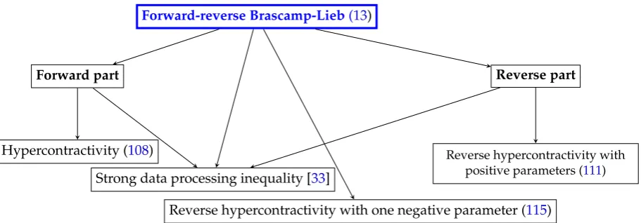
Forward-reverse Brascamp-Lieb(13)

Forward part

Strong data processing inequality [33]

Reverse hypercontractivity with one negative parameter (115) Reverse part

Hypercontractivity (108) _{Reverse hypercontractivity with}

positive parameters (111)

Figure 1. The forward-reverse Brascamp-Lieb inequality generalizes several other functional inequalities/information theoretic inequalities. For more discussions on these relations see the extended version [7].

Theorem 2. Consider b1, . . . ,bl,c1, . . . ,cm,D∈(0,∞). Let E1, . . . ,El,E1, . . . ,Embe Euclidean spaces, and letBji: Ei→Ejbe a linear map for each i∈ {1, . . . ,l}and j∈ {1, . . . ,m}. Then, for all continuous functions

fj:Ej →[0,+∞), gi: Ei→[0,∞)satisfying l

∏

gbi

i (xi)≤ m

∏

f_jcj l

∑

Bjixi !

, ∀x1, . . . ,xl, (15)

we have

l

∏

Z

gi bi

≤D m

∏

Z

fj cj

, (16)

if and only if for all centered Gaussian functions f1, . . . ,fm,g1, . . . ,glsatisfying(15), we have(16). 75

As mentioned, in the literature on the forward or the reverse Brascamp-Lieb inequalities, it is 76

known that a certain geometric condition (5) ensures that the best constant equals 1. Next, we also 77

identify a particular case where the best constant in theforward-reverseinequality equals 1: 78

Theorem 3. Let l be a positive integer, and let M := (mji)1≤j≤l,1≤i≤l be an orthogonal matrix. For any nonnegative continuous functions(fj)lj=1(gi)li=1onRsuch that

l

∏

gi(xi)≤ l

∏

fj l

∑

mjixi !

, ∀xl ∈Rl, (17)

we have

l

∏

gi(x)dx≤ l

∏

fj(x)dx. (18)

The rest of the paper is organized as follows: Section2defines notation and reviews some basic 79

theory of convex duality. Section3proves Theorem1and also presents its extensions to the settings 80

of noncompact spaces or general reverse channels. Section4proves the Gaussian optimality in the 81

entropic formulation, under a certain “non-degenerate” assumption where the linear mapsBji’s are 82

argument in AppendixFlets the noise vanish, which, combined with the equivalence between the 84

functional and entropic formulations, establishes Theorem2and Theorem3. 85

2. Review of the Legendre-Fenchel Duality Theory 86

Our proof of the equivalence of the functional and the entropic inequalities uses the 87

Legendre-Fenchel duality theory, a topic from convex analysis. Before getting into that, a recap 88

of some basics on the duality of topological vector spaces seems appropriate. Unless otherwise 89

indicated, we assume Polish spaces and Borel measures6. Of course, this covers the cases of Euclidean 90

and discrete spaces (endowed with the Hamming metric, which induces the discrete topology, making 91

every function on the discrete set continuous), among others. Readers interested in discrete spaces 92

only may refer to the (much simpler) argument in [47] based on the KKT condition. 93

Notation1. LetX be a topological space. 94

• Cc(X)denotes the space of continuous functions onX with a compact support; 95

• C0(X)denotes the space of all continuous functions f onX that vanish at infinity (i.e. for any 96

e>0 there exists a compact setK ⊆ X such that|f(x)|<eforx∈ X \ K); 97

• Cb(X)denotes the space of bounded continuous functions onX; 98

• M(X)denotes the space of finite signed Borel measures onX; 99

• P(X)denotes the space of probability measures onX. 100

We considerCc,C0andCbas topological vector spaces, with the topology induced from the sup 101

norm. The following theorem, usually attributed to Riesz, Markov and Kakutani, is well-known in 102

functional analysis and can be found in, e.g. [48][49]. 103

Theorem 4(Riesz-Markov-Kakutani). IfX is a locally compact,σ-compact Polish space, the dual7of both 104

Cc(X)and C0(X)isM(X). 105

Remark1. The dual space ofCb(X)can be strictly larger thanM(X), since it also contains those linear 106

functionals that depend on the “limit at infinity” of a functionf ∈Cb(X)(originally defined for those 107

f that do have a limit at infinity, and then extended to the wholeCb(X)by the Hahn-Banach theorem; 108

see e.g. [48]). 109

Of course, anyµ∈ M(X)is a continuous linear functional onC0(X)orCc(X), given by f 7→

Z

fdµ (19)

where f is a function inC0(X)orCc(X). As is well known, Theorem4states that the converse is also true under mild regularity assumptions on the space. Thus, we can view measures as continuous linear functionals on a certain function space;8this justifies the shorthand notation

µ(f):= Z

fdµ (20)

which we employ in the rest of the paper. This viewpoint is the most natural for our setting since in 110

the proof of the equivalent formulation of the forward-reverse Brascamp-Lieb inequality we shall use 111

the Hahn-Banach theorem to show the existence of certain linear functionals. 112

6 _{A Polish space is a complete separable metric space. It enjoys several nice properties that we use heavily in this section,}

including Prokhorov theorem and Riesz-Kakutani theorem (the latter is related to the fact that every Borel probability measure on a Polish space is inner regular, hence a Radon measure). Short introductions on the Polish space can be found in e.g. [37][46].

7 _{The dual of a topological vector space consists of all continuous linear functionals on that space, which is naturally also}

topological vector space (with the weak∗topology).

8 _{In fact, some authors prefer to construct measure theory bydefininga measure as a linear functional on a suitable measure}

Definition1. LetΛ: Cb(X) → (−∞,+∞] be a lower semicontinuous, proper convex function. Its Legendre-Fenchel transformΛ∗:C_b(X)∗ →(−∞,+∞]is given by

Λ∗_{(`):= sup} u∈Cb(X)

[`(u)−Λ(u)]. (21)

Letνbe a nonnegative finite Borel measure on a Polish spaceX, and define the convex functional

onCb(X):

Λ(f):=logν(exp(f)) (22)

=log

Z

exp(f)dν. (23)

Then, note that the relative entropy has the following alternative definition: for anyµ∈ M(X),

D(µkν):= sup f∈C_b(X)

[µ(f)−Λ(f)] (24)

which agrees with the more familiar definitionD(µkν):=µ(logd_dµ

ν)whenνis a probability measure,

113

by the Donsker-Varadhan formula (c.f. [46, Lemma 6.2.13]). Ifµis not a probability measure, then 114

D(µkν)as defined in (24) is+∞. 115

Given a bounded linear operatorT:Cb(Y)→Cb(X), the dual operatorT∗:Cb(X)∗→Cb(Y)∗is defined in terms of

T∗µX:Cb(Y)→R;

f 7→µX(T f), (25)

for anyµX∈Cb(X)∗. SinceP(X)⊆ M(X)⊆Cb(X)∗,Tis said to be aconditional expectation operator 116

ifT∗P∈ P(Y)for anyP∈ P(X). The operatorT∗is defined as the dual of a conditional expectation 117

operatorT, and in a slight abuse of terminology, is said to be arandom transformationfromX toY. 118

For example, in the notation of Theorem1, ifg∈ Cb(Y)andQY|X is a random transformation 119

fromX toY, the quantityQY|X(g)is a function onX, defined by taking the conditional expectation. 120

Also, ifPX ∈ P(X), we writePX→QY|X →PYto indicate thatPY∈ P(Y)is the measure induced on 121

Y by applyingQY|XtoPX. 122

Remark 2. From the viewpoint of category theory (see for example [51][52]), Cb is a functor 123

from the category of topological spaces to the category of topological vector spaces, which is 124

contra-variant because for any continuous, φ: X → Y (morphism between topological spaces), 125

we haveCb(φ):Cb(Y)→Cb(X),u7→u◦f whereu◦φdenotes the composition of two continuous 126

functions, reversing the arrows in the maps (i.e. the morphisms). On the other hand,Mis a covariant 127

functor andM(φ):M(X) → M(Y),µ 7→ µ◦φ−1, whereµ◦φ−1(B) := µ(φ−1(B))for any Borel 128

measurableB ⊆ Y. “Duality” itself is a contra-variant functor between the category of topological 129

spaces (note the reversal of arrows in Fig.2). Moreover,Cb(X)∗ =M(X)andCb(φ)∗=M(φ)ifX 130

andY are compact metric spaces andφ:X → Y is continuous. Definition2can therefore be viewed 131

as the special case whereφis the projection map: 132

Definition2. Supposeφ:Z1× Z2→ Z1,(z1,z2)7→z1is the projection to the first coordinate. 133

• Cb(φ):Cb(Z1)→Cb(Z1× Z2)is called acanonical map, whose action is almost trivial: it sends a 134

function ofzito itself, but viewed as a function of(z1,z2). 135

• M(φ):M(Z1× Z2)→ M(Z1)is calledmarginalization, which simply takes a joint distribution 136

to a marginal distribution. 137

The Fenchel-Rockafellar duality (see [37, Theorem 1.9], or [53] in the case of finite dimensional 138

Theorem 5. Assume that A is a topological vector space whose dual is A∗. Let Θj: A → R∪ {+∞},

j=0, 1, . . . ,k, for some positive integer k. Suppose there exist some(uj)kj=1and u0:=−(u1+· · ·+uk)such that

Θj(uj)<∞, j=0, . . . ,k (26) andΘ0is upper semicontinuous at u0. Then

− inf `∈A∗

" _k

∑

Θ∗ j(`)

#

= inf u1,...,uk∈A

"

Θ0 −

k

∑

uj !

+ k

∑

Θj(uj) #

. (27)

For completeness, we provide a proof of this result, which is based on the Hahn-Banach theorem 140

(Theorem6) and is similar to the proof of [37, Theorem 1.9]. 141

Proof. Letm0be the right side of (27). The≤part of (27) follows trivially from the (weak) min-max inequality since

m0= inf u0,...,uk∈A

sup `∈A∗

( _k

∑

Θj(uj)−`( k

∑

uj) )

(28)

≥ sup `∈A∗

inf u0,...,uk∈A

( _k

∑

Θj(uj)−`( k

∑

uj) )

(29)

=− inf `∈A∗

" _k

∑

Θ∗ j(`)

#

. (30)

It remains to prove the≥part, and it suffices to assume without loss of generality thatm0>−∞. Note that (26) also implies thatm0<+∞. Define convex sets

Cj:={(u,r)∈ A×R: r>Θj(u)}, j=0, . . . ,k; (31)

B:={(0,m)∈A×R: m≤m0}. (32)

Observe that these are nonempty sets because of (26). AlsoC0has nonempty interior by the assumption thatΘ0is upper semicontinuous atu0. Thus, the Minkowski sum

C:=C0+· · ·+Ck (33) is a convex set with a nonempty interior. Moreover, C∪B = ∅. By the Hahn-Banach theorem (Theorem6), there exists(`,s)∈ A∗×Rsuch that

sm≤` k

∑

uj !

+s k

∑

rj. (34)

For anym ≤ m0and(uj,rj) ∈ Cj, j = 0, . . . ,k. From (32) we see (34) can only hold whens ≥ 0. Moreover, from (26) and the upper semicontinuity ofΘ0atu0we see the∑kj=0ujin (34) can take value in a neighbourhood of 0 ∈ A, hences 6= 0. Thus, by dividingson both sides of (34) and setting `← −`/s, we see that

m0≤ inf u0,...,uk∈A

" −`

k

∑

uj !

+ k

∑

Θj(uj) #

(35)

=− " _k

∑

Θ∗ j(`)

#

which establishes≥in (27). 142

Theorem 6(Hahn-Banach). Let C and B be convex, nonempty disjoint subsets of a topological vector space A. 143

1. If the interior of C is non-empty, then there exists`∈ A∗,`6=0such that sup

u∈B

`(u)≤ inf

u∈C`(u). (37)

2. If A is locally convex, B is compact, and C is closed, then there exists`∈ A∗such that sup

u∈B

`(u)< inf

u∈C`(u). (38)

Remark3. The assumption in Theorem6thatChas nonempty interior is only necessary in the infinite 144

dimensional case. However, even ifAin Theorem5is finite dimensional, the assumption in Theorem5

145

thatΘ0is upper semicontinuous atu0is still necessary, because this assumption was not only used in 146

applying Hahn-Banach, but also in concluding thats6=0 in (34). 147

3. The Entropic-Functional Duality 148

In this section we prove Theorem1and some of its generalizations. 149

3.1. CompactX 150

We first state a duality theorem for the case of compact spaces to streamline the proof. Later we 151

show that the argument can be extended to a particular non-compact case.9Our proof based on the 152

Legendre-Fenchel duality (Theorem5) was inspired by the proof of the Kantorovich duality in the 153

theory of optimal transportation (see [37, Chapter 1], where the idea was credited to Brenier). 154

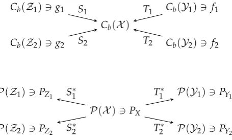
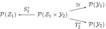
Recall from Section2that a random transformation (a mapping between probability measures) 155

is formally the dual of a conditional expectation operator. SupposePYj|X = T ∗

j, j = 1, . . . ,mand 156

P_Zi|X =S∗i,i=1, . . . ,l.

Cb(X) Cb(Z1)3g1

Cb(Z2)3g2

Cb(Y1)3 f1

Cb(Y2)3 f2 S1

S2

T1

T2

P(X)3PX P(Z₁)3PZ1

P(Z2)3PZ2

P(Y₁)3 PY1

P(Y2)3 PY2

S∗₁

S∗₂

T₁∗

T₂∗

Figure 2.Diagrams for Theorem1. 157

Proof of Theorem1. We can safely assumed=0 below without loss of generality (since otherwise 158

we can always substituteµ1←exp

d c1

µ1). 159

1)⇒2) This is the nontrivial direction which relies on certain (strong) min-max type results. In Theorem5, put10

Θ0:u∈Cb(X)7→ (

0 u≤0;

+∞ otherwise. (39)

Then,

Θ∗

0:π∈ M(X)7→ (

0 π≥0;

+∞ otherwise. (40)

For eachj=1, . . . ,m, set

Θj(u):=cjinf logµj exp 1 cjv

!!

(41)

where the infimum is overv∈Cb(Y)such thatu=Tjv; if there is no suchvthenΘj(u):= +∞ 160

as a convention. Observe that 161

• Θ_jis convex: indeed given arbitraryu0andu1, suppose thatv0andv1respectively achieve 162

the infimum in (41) foru0and u1 (if the infimum is not achievable, the argument still 163

goes through by the approximation and limit argument). Then for anyα ∈ [0, 1],vα := 164

(1−α)v0+αv1satisfiesuα=Tjvαwhereuα:= (1−α)u0+αu1. Thus, the convexity ofΘj 165

follows from the convexity of the functional in (23); 166

• Θ_j(u)>−∞for anyu∈Cb(X). Otherwise, for anyPXandPYj :=T ∗

jPXwe have D(PYjkµj) =sup

v

{PYj(v)−logµj(exp(v))} (42)

=sup v

{PX(Tjv)−logµj(exp(v))} (43)

= sup u∈C_b(X)

(

PX(u)− 1 cjΘj

(cju) )

(44)

= +∞ (45)

which contradicts the assumption that∑m

j=1cjD(PYjkµj)<∞in the theorem; 167

• From the steps (42)-(44), we seeΘ∗_j(π) = cjD(Tj∗πkµj)for any π ∈ M(X), where the 168

definition ofD(·kµj)is extended using the Donsker-Varadhan formula (that is, it is infinite 169

when the argument is not a probability measure). 170

Finally, for the given(PZ_i)l_i=1, choose

Θm+1: u∈Cb(X)7→ (

∑l

i=1PZi(wi) ifu=∑

l

i=1Siwifor somewi∈Cb(Zi);

+∞ otherwise. (46)

Notice that 171

• Θ_m+1is convex; 172

• Θm+1is well-defined (that is, the choice of(wi)in (46) is inconsequential). Indeed if(wi)li=1 is such that∑l

i=1Siwi =0, then l

∑

PZ_i(wi) = l

∑

S∗_iPX(wi) (47)

= l

∑

PX(Siwi) (48)

=0, (49)

where PX is such thatS∗_iPX = PZ_i,i = 1, . . . ,l, whose existence is guaranteed by the 173

assumption of the theorem. This also shows thatΘm+1>−∞. 174

•

Θ∗

m+1(π):=sup u

{π(u)−Θm+1(u)} (50)

= sup w1,...,wl

(

π l

∑

Siwi !

− l

∑

PZ_i(wi) )

(51)

= sup w1,...,wl

( _l

∑

S∗_iπ(wi)− l

∑

PZ_i(wi) )

(52)

= (

0 ifS∗_iπ=PZ_i, i=1, . . . ,l;

+∞ otherwise. (53)

Invoking Theorem5(where theujin Theorem5can be chosen as the constant functionuj≡1, j=1, . . . ,m+1):

inf

π:π≥0,S∗_iπ=P_Zi

m

∑

cjD(Tj∗πkµj)

=− inf

vm_,wl_:∑m

j=1Tjvj+∑il=1Siwi≥0 "_m

∑

cjlogµj exp 1 cjvj

!! +

l

∑

PZ_i(wi) #

(54)

wherevmdenotes the collection of the functionsv1, . . . ,vm, and similarly forwl. Note that the left side of (54) is exactly the right side of (14). For anye>0, choosevj∈ Cb(Yj),j=1, . . . ,m andwi ∈Cb(Zi),i=1, . . . ,lsuch that∑jm=1Tjvj+∑li=1Siwi ≥0 and

e− m

∑

cjlogµj exp 1 cjvj

!! −

l

∑

PZi(wi)> inf

π:π≥0,S∗_iπ=P_Zi m

∑

cjD(Tj∗πkµj) (55)

Now invoking (13) with fj :=exp_c1

jvj

,j=1, . . . ,mandgi :=exp−1 biwi

,i=1, . . . ,l, we upper bound the left side of (55) by

e− l

∑

bilogνi(gi) + l

∑

biPZ_i(loggi)≤e+ l

∑

biD(PZ_ikνi) (56)

where the last step follows by the Donsker-Varadhan formula. Therefore (14) is established since 175

2)⇒1) Sinceνiis finite andgiis bounded by assumption, we haveνi(gi)<∞,i=1, . . . ,l. Moreover (13) is trivially true whenνi(gi) =0 for somei, so we will assume below thatνi(gi)∈(0,∞)for eachi. DefinePZ_i by

dPZ_i dνi

= gi νi(gi)

, i=1, . . . ,l. (57)

Then for anye>0,

l

∑

bilogνi(gi) = l

∑

bi[PZi(loggi)−D(PZikνi)] (58)

< m

∑

cjPYj(logfj) +e−

m

∑

cjD(PYjkµj) (59)

≤e+ m

∑

cjlogµj(fj) (60)

where 177

• (59) uses the Donsker-Varadhan formula, and we have chosenPX,PYj :=T ∗

jPX,j=1, . . . ,m such that

l

∑

biD(PZikνi)>

m

∑

cjD(PYjkµj)−e (61)

• (60) also follows from the Donsker-Varadhan formula. 178

The result follows sincee>0 can be arbitrary. 179

180

Remark4. Condition iv) in the theorem imposes a rather strong assumption on(Si): for simplicity, 181

consider the case where|X |,|Zi| < ∞. Then Condition iv) assumes that for any(PZ_i), there exists 182

PXsuch thatPZ_i =S∗_iPX. This assumption is certainly satisfied when(Si)are induced by coordinate 183

projections; the case ofl=1 andP_Z|Xbeing a reverse erasure channel gives a simple example where 184

PZ|Xis not a deterministic map. 185

Next we give a generalization of Theorem1which alleviates the restriction on(Si): 186

Theorem 7. Theorem1continues to hold if Condition iv) therein is weakened to the following: 187

• For any PXsuch that D(S∗iPXkνi)<∞, i=1, . . . ,l, there existsP˜Xsuch that S∗iP˜X =S∗iPXfor each i 188

and∑m_j=1cjD(T_j∗PX˜ kµj)<∞for each j. 189

and the conclusion of the theorem will be replaced by the equivalence of the following two statements: 190

1. For any nonnegative continuous functions(gi),(fj)bounded away from0and such that l

∑

biSiloggi≤ m

∑

cjTjlogfj (62)

we have

inf

(g˜i): ∑li=1biSilog ˜gi≥∑li=1biSiloggi

l

∏

ν_ibi(gi˜)≤exp(d) m

∏

µ c_j

2. For any(PX)such that D(S∗_iPXkνi)<∞, i=1, . . . ,l, l

∑

biD(S∗iPXkνi) +d≥ inf ˜

PX:S∗iP˜X=S∗iPX

m

∑

cjD(Tj∗P˜Xkµj). (64)

In AppendixAwe show that Theorem7indeed recovers Theorem1for the more restricted class 191

of random transformations. 192

Proof. Here we mention the parts of the proof that need to be changed: upon specifying(fj)and(gi) right after (55), we select(g˜i)such that

l

∑

biSilog ˜gi ≥ l

∑

biSiloggi (65)

l

∑

bilogνi(g˜i)≤ m

∑

cjlogµj(fj) +e. (66)

Then, in lieu of (67), we upper-bound the left side of (55) by

2e− l

∑

bilogνi(g˜i) + l

∑

biPZi(log ˜gi)≤2e+

l

∑

biD(PZikνi) (67)

which establishes the 1)⇒2) part. For the other direction, for eachi∈ {1, 2, . . . ,l}define

Λi(u):= inf ˜

gi>0 :biSilog ˜gi=u

bilogνi(g˜i). (68)

Then following essentially the same proof as that ofΘjin (41), we see thatΛiis proper convex and

Λ∗

i(π) =biD(S∗iπkµj). (69) Moreover let

Λl+1(u):= (

0 ifu=−∑biSiloggi;

+∞ otherwise. (70)

ThenΛ∗_l+1(π) =−∑biS∗iπ(loggi). Using the Legendre-Fenchel duality we see that for anye>0,

inf

(g˜i):∑li=1biSilog ˜gi≥∑li=1biSiloggi

l

∑

bilogνi(gi˜)

= inf u₁,...,u_l+1

(

Θ0 −

l+1

∑

ui !

+ l+1

∑

Λi(ui) )

(71)

=sup

π

( −

l+1

∑

Θ∗ i(π)

)

(72)

=sup

π≥0

( −

l+1

∑

Θ∗ i(π)

)

(73)

=sup

π≥0

( _l

∑

biSi∗π(loggi)− l

∑

biD(S∗iπkνi) )

(74)

≤ l

∑

biS∗_iPX(loggi)− l

∑

≤ m

∑

cjTj∗PX˜ (logfj)− m

∑

cjD(Tj∗PX˜ kµj) +2e (76)

≤2e+ m

∑

cjlogµj(fj) (77)

where 193

• To see (75) we note that the sup in (74) can be restricted toπwhich is a probability measure, since 194

otherwise the relative entropy terms in (74) are+∞by its definition via the Donsker-Varadhan 195

formula. Then we selectPXsuch that (75) holds. 196

• In (76), we have chosen ˜PXsuch that

S_i∗PX˜ =S∗_iPX, 1≤i≤l; (78) l

∑

biD(S∗_iPX)> m

∑

cjD(T_j∗PX˜ kµj)−e, (79)

and then applied the assumption (62). The result follows sincee>0 can be arbitrary. 197

198

Remark5. The infimum in (14) is in fact achievable: For any(PZi), there exists aPXthat minimizes 199

∑m

j=1cjD(PYjkµj)subject to the constraintsS ∗

iPX =PZi,i=1, . . .m, wherePYj :=T ∗

jPX,j=1, . . . ,m. 200

Indeed, since the singleton{PZ_i}is weak∗-closed andS∗_i is weak∗-continuous11, the setTl

i=1(Si∗)−1PZi 201

is weak∗-closed in M(X); hence its intersection withP(X) is weak∗-compact in P(X), because 202

P(X)is weak∗-compact by (a simple version for the setting of a compact underlying spaceX of) 203

the Prokhorov theorem [54]. Moreover, by the weak∗-lower semicontinuity ofD(·kµj)(easily seen 204

from the variational formula/Donsker-Varadhan formula of the relative entropy, cf. [55]) and the 205

weak∗-continuity ofT_j∗,j=1, . . . ,m, we see that∑m

j=1cjD(Tj∗PXkµj)is weak∗-lower semicontinuous 206

inPX, and hence the existence of a minimizingPXis established. 207

Remark6. Abusing the terminology from min-max theory, Theorem1may be interpreted as a “strong 208

duality” result which establishes the equivalence of two optimization problems. The 1)⇒2) part is the 209

non-trivial direction which requires regularity on the spaces. In contrast, the 2)⇒1) direction can be 210

thought of as a “weak duality” which establishes only a partial relation but holds for more general 211

spaces. 212

3.2. NoncompactX 213

Our proof of 1)⇒2) in Theorem1makes use of the Hahn-Banach theorem, and hence relies 214

crucially on the fact that the measure space is the dual of the function space. Naively, one might want to 215

extend the the proof to the case oflocally compactX by consideringC0(X)instead ofCb(X), so that the 216

dual space is stillM(X). However, this would not work: consider the case whenX =Z1×, . . . ,×Zl 217

and eachSi is the canonical map. ThenΘm+1(u)as defined in (46) is+∞unlessu ≡ 0 (because 218

u ∈ C0(X) requires thatu vanishes at infinity), thusΘ∗m+1 ≡ 0. Luckily, we can still work with 219

Cb(X); in this case`∈Cb(X)∗may not be a measure, but we can decompose it into`=π+Rwhere 220

π∈ M(X)andRis a linear functional “supported at infinity”. Below we use the techniques in [37, 221

Chapter 1.3] to prove a particular extension of Theorem1to a non-compact case. 222

Theorem 8. Theorem1still holds if 223

• The assumption thatX is a compact metric space is relaxed to the assumption that it is a locally compact 224

andσ-compact Polish space; 225

• X =_∏l_i=1Z_iand Si:Cb(Zi)→Cb(X), i=1, . . . ,l are canonical maps (see Definition2). 226

Proof. The proof of the “weak duality” part 2)⇒1) still works in the noncompact case, so we only need to explain what changes need to be made in the proof of 1)⇒2) part. LetΘ0be defined as before, in (39). Then for any`∈Cb(X)∗,

Θ∗

0(`) =sup u≤0

`(u) (80)

which is 0 if`is nonnegative (in the sense that`(u)≥0 for everyu≥0), and+∞otherwise. This 227

means that when computing the infimum on the left side of (27), we only need to take into account of 228

those nonnegative`. 229

Next, letΘm+1be also defined as before. Then directly from the definition we have

Θ∗

m+1(`) = (

0 if`(_∑iSiwi) =∑iPZi(wi), ∀wi∈Cb(Zi),i=1, . . .l;

+∞ otherwise. (81)

For any`∈C∗<sub>b</sub>(X). Generally, the condition in the first line of (81) does not imply that`is a measure. However, if`is also nonnegative, then using a technical result in [37, Lemma 1.25] we can further simplify:

Θ∗

m+1(`) = (

0 if`∈ M(X)andS∗<sub>i</sub>`=PZi, i=1, . . . ,l;

+∞ otherwise. (82)

This further shows that when we compute the left side of (27) the infimum can be taken over`which 230

is a coupling of(PZi). In particular, if`is a probability measure, thenΘ ∗

j(`) =cjD(Tj∗`kµj)still holds 231

with theΘjdefined in (41),j=1, . . . ,m. Thus the rest of the proof can proceed as before. 232

Remark7. The second assumption is made in order to achieve (82) in the proof. 233

4. Gaussian Optimality 234

Recall that the conventional Brascamp-Lieb inequality and its reverse ((1) and (2)) state that 235

centered Gaussian functions exhaust such inequalities, and in particular, verifying those inequalities is 236

reduced to a finite dimensional optimization problem (only the covariance matrices in these Gaussian 237

functions are to be optimized). In this section we show that similar results hold for the forward-reverse 238

Brascamp-Lieb inequality as well. Our proof uses the rotational invariance argument mentioned in 239

Section1. Since the forward-reverse Brascamp-Lieb inequality has dual representations (Theorem8), 240

in principle, the rotational invariance argument can be applied either to the functional representation 241

(as in Lieb’s paper [29]) or the entropic representation (as in Geng-Nair [45]). Here, we adopt the latter 242

approach. We first consider a certain “non-degenerate” case where the existence of an extremizer is 243

guaranteed. Then, Gaussian optimality in the general case follows by a limiting argument (AppendixF), 244

establishing Theorem2and Theorem3. 245

4.1. Non-Degenerate Forward Channels 246

This subsection focuses on the following case: 247

Assumption1. • Fix Lebesgue measures(µj)m_j=1and Gaussian measures(νi)l_i=1onR; 248

• non-degenerate (Definition3below) linear Gaussian random transformation(PYj|X)

m

j=1(where 249

• (Si)li=1are induced by coordinate projections; 251

• positive(cj)and(bi). 252

Definition3. We say(QY1|X, . . . ,QYm|X)isnon-degenerateif eachQYj|X=0is annj-dimensional Gaussian 253

distribution with invertible covariance matrix. 254

Given Borel measuresPX_ionR,i=1, . . . ,l, define

F0((PX_i)):=inf PX

m

∑

cjD(PYjkµj)−

l

∑

biD(PXikνi) (83)

where the infimum is over Borel measuresPXthat has(PXi)as marginals. Note that (83) is well-defined 255

since the first term cannot be+∞under the non-degenerate assumption, and the second term cannot 256

be−∞. The aim of this subsection is to prove the following: 257

Theorem 9. sup_(P

Xi)F0((PXi)), where the supremum is over Borel measures PXionR, i=1, . . . ,l, is achieved 258

by some Gaussian(PXi)

l

i=1, in which case the infimum in(83)is achieved by some Gaussian PX. 259

Naturally, one would expect that Gaussian optimality can be established when(µj)mj=1and(νi)li=1 260

are either Gaussian or Lebesgue. We made the assumption that the former is Lebesgue and the latter is 261

Gaussian so that certain technical conditions can be justified more easily. More precisely, the following 262

observation shows that we can regularize the distributions by a second moment constraint for free: 263

Proposition 10. sup_(P

Xi)F0((PXi))is finite and there existσ 2

i ∈(0,∞), i=1, . . . ,l such that it equals sup

(P_Xi):E[Xi2]≤σi2

F0((PXi)). (84)

Proof. when µj is Lebesgue and PYj|X is non-degenerate, D(PYjkµj) = −h(PYj) ≤ −h(PYj|X) is 264

bounded above (in terms of the variance of additive noise ofPYj|X). Moreover,D(PXikνi)≥0 whenνi 265

is Gaussian, so sup_(P

Xi)F0((PXi))<∞. Further, choosing(PXi) = (νi)and using the covariance matrix 266

to lower bound the first term in (83) shows that sup_(P

Xi)F0((PXi))>−∞. 267

To see (84), notice that

D(PX_ikνi) =D(PXikν 0

i) +E[ıν_i0kνi(X)] (85)

=D(PXikν 0

i) +D(νi0kνi) (86)

≥D(ν_i0kνi) (87)

where ν0_i is a Gaussian distribution with the same first and second moments as Xi ∼ PXi. Thus 268

D(PX_ikνi)is bounded below by some function of the second moment ofXiwhich tends to∞as the 269

second moment ofXitends to∞. Moreover, as argued in the preceding paragraph the first term in 270

(83) is bounded above by some constant depending only on(PY_j|X). Thus, we can chooseσi2 > 0, 271

i = 1, . . . ,llarge enough such that ifE[Xi2] > σi2for some ofithen F0((PXi)) < sup(P_Xi)F0((PXi)), 272

irrespective of the choices ofPX1, . . . ,PXi−1,PXi+1, . . . ,PXl. Then theseσ1, . . . ,σlare as desired in the 273

proposition. 274

The non-degenerate assumption ensures that the supremum is achieved: 275

Proposition 11. Under Assumption1, 276

2. If(P_Yj|Xl)m_j=1are non-degenerate (Definition3), then the supremum in(84)is achieved by some Borel 278

(PX_i)_il₌₁. 279

The proof of Proposition 11 is given in Section E. After taking care of the existence of the 280

extremizers, we get into the tensorization properties which are the crux of the proof: 281

Lemma 12. Fix(P

X_i(1)),(PX(_i2)),(µj),(Tj),(cj)∈[0,∞)

m_{, and let S}

jbe induced by coordinate projections. Then

inf P

X(1,2):S ∗⊗2

i PX(1,2)=PX_i(1)×PX(_i2)

m

∑

cjD(P Y_j(1,2)kµ

⊗2 j ) =

∑

t=1,2 m

∑

cj inf

P X(t):S

∗

iP_X(t)=P

X(_it)

D(P

Y_j(t)kµj) (88)

where for each j,

P

Y_j(1,2):=T ∗⊗2

j PX(1,2) (89)

on the left side and

P_Y(t)

j

:=T_j∗⊗2P_X(t) (90)

on the right side, t=1, 2. 282

Proof. We only need to prove the nontrivial≥part. For anyP_X(1,2)on the left side, chooseP_X(t)on the

right side by marginalization. Then

D(P_Y(1,2)

j

kµ⊗2_j )−

∑

D(P_Y(t)

j

kµj) =I(Y_j(1);Y_j(2)) (91)

≥0 (92)

for eachj. 283

We are now ready to show the main result of this section. 284

Proof of Theorem9. 1. Assume that(P_X(1)

i

)and(P_X(2)

i

)are maximizers ofF0(possibly equal). Let P_X1,2

i :

=P

X(_i1)×PX(_i2). Define

X+ := √1 2

X(1)+X(2); (93)

X− := √1 2

X(1)−X(2). (94)

Define(Y_j+)and(Y_j−)analogously. ThenY_j+|{X+ =x+,X−=x−} ∼QYj|X=x+ is independent 285

ofx−andY_j−|{X+=x+,X− =x−} ∼QY_j|X=x−is independent ofx+. 286

2. Next we perform the same algebraic expansion as in the proof of tensorization:

2

∑

F0

P_X(t)

i l

i=1 !

= inf

P X(1,2):S

∗⊗2

j PX(1,2)=PX(_j1,2)

∑

cjD(P_Y(1,2)

j

kµ⊗2_j )−

∑

biD(P_X(1,2)

i

kν_i⊗2) (95)

= inf

P_X+_X−:S_j∗⊗2P_X+_X−=P_X+

j X−j

∑

cjD(PY_j+Y_j−kµ ⊗2 j )−

∑

i

biD(PX+_i X−_i kν ⊗2 i )

≤ inf P_X+_X−:S_j∗⊗2P_X+_X−=P_X+

j X − j

∑

D(P_Y+

j kµj) +D(PYj−|X+kµj|PX

+) −

∑

D(P_X+

i kνi) +D(PX

−

i |X

+

i kνi|PX

+ i ) i (97) ≤

∑

D(P_Y?+

j

kµj) +D(P_Y?−

j |X+

kµj|P_X?+)

−

∑

bihD(P_X?+

i

kνi) +D(P_X?−

i |X+

kνi|P_X?+)

i

(98)

=F0

P_X?+

i l

i=1 + Z F0 P_X?−

i |X+ l

i=1

dP_X?+ (99)

≤ 2

∑

F0

P_X(t)

i l

i=1 !

(100)

where 287

• (95) uses Lemma12. 288

• (97) is because of the Markov chainY_j+−X+−Y_j−(for any coupling). 289

• In (98) we selected a particular instance of couplingP_X+_X−, constructed as follows: first we select an optimal couplingPX+ for given marginals(P_X+

i ). Then, for anyx

+_{= (x}+

i )li=1, let PX−_|X+_=x+ be an optimal coupling of(P_X−

i |X

+

i =x

+

i ).

12 _{With this construction, it is apparent}

thatX_i+−X+−X_i−and hence D(P_X−

i |X

+

i kνi|PX

+

i ) =D(PX−i |X+kνi|PX

+). (101)

• (99) is because in the above we have constructed the coupling optimally. 290

• (100) is because(P_X(t)

i)maximizesF0,t=1, 2. 291

3. Thus in the expansions above, equalities are attained throughout. Using the differentiation technique as in the case of forward inequality, for almost all(bi),(cj), we have

D(P_X−

i |X

+

i kνi|PX

+

i ) =D(PX

+

i kνi) (102)

=D(P_X−

i kνi), ∀i (103)

where (103) is because by symmetry we can perform the algebraic expansions in a different way to 292

show that(P_X−

i )is also a maximizer ofF0. ThenI(X

+

i ;X −

i ) =D(PX−_i |X_i+kνi|PX+_i )−D(PX_i−kνi) = 293

0, which, combined with I(X_i(1);X_i(2)), shows that X(_i1)andX(_i2)are Gaussian with the same 294

covariance. Lastly, using Lemma12 and the doubling trick one can show that the optimal 295

coupling is also Gaussian. 296

297

4.2. A Geometric Forward-Reverse Brascamp-Lieb Inequality 298

In this section we give a sketch of the proof of Theorem3which is simple but certain ‘technicalities” 299

are not justified. A detailed proof is deferred to AppendixF. 300

Proof Sketch for Theorem3. By duality (Theorem8) it suffices to prove the corresponding entropic inequality. The Gaussian optimality result in Theorem9assumed Gaussian reference measures on the output and non-degenerate forward channels in order to simplify the proof of the existence of

12 _{For a justification that we can select optimal couplingP}

minimizers; however, supposing that Gaussian optimality extends beyond those technical conditions, then we see that it suffices to prove that for any centered Gaussian(PXi),

l

∑

h(PX_i)≤sup P_Xl

l

∑

h(PY_j) (104)

where the supremum is over GaussianP_Xl with the marginalsPX₁, . . . ,PX_l, andYj :=∑l_i=1mjiXi. Let

ai :=E[Xi2]and choosePXl =∏l_i=1PX_i, we see (104) holds if

l

∑

logai≤ l

∑

log l

∑

m2_jiai !

, ∀ai >0,i=1, . . . ,l, (105)

where(ai)are the eigenvalues and∑l i=1mjiai

l

i=1are the diagonal entries of the matrix

Mdiag(ai)1≤i≤lM>. (106) Therefore (105) holds.

301

5. Relation to Hypercontractivity and Its Reverses 302

As alluded before and illustrated by Figure1, the forward-reverse Brascamp-Lieb inequality 303

generalizes several other inequalities from functional analysis and information theory; A more 304

complete discussion on these relationships can be found in [7]. In this section, we focus on 305

hypercontractivity, and show how its three cases all follow from Theorem 1. Among these, the 306

case in Section5.3can be regarded as an instance of the forward-reverse inequality that cannot be 307

reduced to either the forward or the reverse inequality alone. It is also interesting to note that, from 308

the viewpoint of the forward-reverse Brascamp-Lieb inequality, in each of the three special cases there 309

ought to be three functions involved in the functional formulation; but the optimal choice of one 310

function can be computed from the other two. Therefore the conventional functional formulations 311

of the three cases of hypercontractivity involve only two functions, making it non-obvious to find a 312

unifying inequality. 313

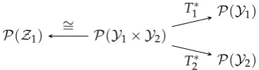
5.1. Hypercontractivity 314

P(Y1× Y2) P(Z1)

P(Y1)

P(Y2) ∼

=

T₁∗

T₂∗

Figure 3.Diagram for hypercontractivity

Fix a joint probability distributionQY1Y2 and nonnegative continuous functionsF1andF2onY1

andY2, respectively, both bounded away from 0. In Theorem1, takel←1,m←2,b1←1,d ←0, f1←F

1

c₁

1 , f2←F

1

c₂

2 ,ν1←QY1Y2,µ1←QY1,µ2←QY2. Also, putZ1=X= (Y1,Y2), and letT1andT2

be the canonical maps (Definition2). The constraint (12) translates to

and the optimal choice ofg1is when the equality is achieved. We thus obtain the equivalence between13 kF1k1

c₁kF2kc1₂ ≥E[F1(Y1)F2(Y2)], ∀F1∈ L

1

c_1(Q

Y1),F2∈ L 1

c_2(Q

Y2) (108)

and

∀PY1Y2, D(PY1Y2kQY1Y2)≥c1D(PY1kQY1) +c2D(PY2kQY2). (109)

This equivalence can also be obtained from Theorem1. By Hölder’s inequality, (108) is equivalent to 315

saying that the norm of the linear operator sendingF1∈ L

1

c_1(QY

1)toE[F1(Y1)|Y2=·]∈ L 1 1−c_2(QY

2)

316

does not exceed 1. The interesting case is₁₋1_c

2 >

1

c1, hence the name hypercontractivity. The equivalent

317

formulation of hypercontractivity was shown in [41] using a different proof via the method of 318

types/typicality, which requires that|Y₁|,|Y₂|<∞. In contrast, the proof based on the nonnegativity 319

of relative entropy removes this constraint, allowing one to prove Nelson’s Gaussian hypercontractivity 320

from the information-theoretic formulation (see [7]). 321

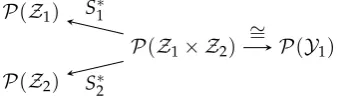
5.2. Reverse Hypercontractivity (Positive Parameters14) 322

P(Z1× Z2) P(Z1)

P(Z2)

P(Y1) S∗₁

S∗₂

∼ =

Figure 4.Diagram for reverse hypercontractivity

LetQZ1Z2 be a given joint probability distribution, and letG1andG2be nonnegative functions on

Z1andZ2, respectively, both bounded away from 0. In Theorem1, takel←2,m←1,c1←1,d←0, g1←G

1

b₁

1 ,g2←G

1

b₂

2 ,µ1←QZ1Z2,ν1←QZ1,ν2←QZ2. Also, putY1=X= (Z1,Z2), and letS1and

S2be the canonical maps (Definition2). Note that the constraint (12) translates to

f1(z1,z2)≥G1(z1)G2(z2), ∀z1,z2. (110) and the equality case yields the optimal choice of f1 for (13). By Theorem1we thus obtain the equivalence between

kG1k1

b₁kG2kb1₂ ≤E[G1(Z1)G2(Z2)], ∀G1,G2 (111)

and

∀PZ1,PZ2,∃PZ1Z2, D(PZ1Z2kQZ1Z2)≤b1D(PZ1kQZ1) +b2D(PZ2kQZ2). (112)

Note that in this setup, ifZ1andZ2 are finite, then Condition iv) in Theorem1is equivalent to 323

QZ₁Z2 QZ1×QZ2. The equivalent formulations of reverse hypercontractivity were observed in [56],

324

where the proof is based on the method of types. 325

13 _{By a standard dense-subspace argument, we see that it is inconsequential thatF}

1andF2in (108) are not assumed to be

continuous nor bounded away from zero. It is also easy to see that the nonnegativity ofF1andF2is inconsequential for

(108).

14 _{By “positive parameters” we mean theb}

5.3. Reverse Hypercontractivity (One Negative Parameter15) 326

P(Z1× Y2) P(Z1)

P(Y1)

P(Y2) S∗₁

∼ =

T₂∗

Figure 5.Diagram for reverse hypercontractivity with one negative parameter

In Theorem1, takel ←1,m←2,c1 ←1,d ←0. LetY1 = X= (Z1,Y2), and letS1andT2be the canonical maps (Definition2). Suppose thatQZ₁Y2 is a given joint probability distribution, and

setµ1←QZ1Y2,ν1←QZ1,µ2←QY2 in Theorem1. Suppose thatFandGbe arbitrary nonnegative

continuous functions onY2andZ1, respectively, which are bounded away from 0. Takeg1←G

1

b_1,

f2←F −1

c_{2. in Theorem1. The constraint (12) translates to}

f1(z1,y2)≥G(z1)F(y2), ∀z1,y2. (113) Note that (13) translates to

kGk1

b₁ ≤QY2Z1(f1)Q

c2

Y2(F

−1

c_{2) (114)}

for allF,G, and f1satisfying (113). It suffices to verify (114) for the optimal choice f1=GF, so (114) is reduced to

kFk 1

−c₂kGkb1₁ ≤E[F(Y2)G(Z1)], ∀F,G. (115)

By Theorem1, (115) is equivalent to

∀PZ₁,∃PZ1Y2, D(PZ1Y2kQZ1Y2)≤b1D(PZ1kQZ1) + (−c2)D(PY2kQY2). (116)

Inequality (115) is called reverse hypercontractivity with a negative parameter in [42], where the 327

entropic version (116) is established for|Z1|,|Y2| < ∞using the method of types. Multiterminal 328

extensions of (115) and (116) (called reverse Brascamp-Lieb type inequality with negative parameters 329

in [42]) can also be recovered from Theorem1in the same fashion, i.e., we move all negative parameters 330

to the other side of the inequality so that all parameters become positive. 331

In summary, from the viewpoint of Theorem1, the results in Section5.1,5.2and5.3are degenerate 332

special cases, in the sense that in any of the three cases the optimal choice of one of the functions in (13) 333

can be explicitly expressed in terms of the other functions, hence this “hidden function” disappears in 334

(108), (111) or (115). 335

Acknowledgments: This work was supported in part by NSF Grants CCF-1528132, CCF-0939370 (Center for 336

Science of Information), CCF-1319299, CCF-1319304, CCF-1350595 and AFOSR FA9550-15-1-0180. Jingbo Liu 337

would like to thank Professor Elliott H. Lieb for teaching the Brascamp-Lieb inequality as well as some techniques 338

used in this paper in his graduate class. 339

Author Contributions:All the authors have contributed to the problem formulation, refinement, structuring or 340

editing of the paper. Most of the sections were written by Jingbo Liu. Parts of the sections on the existence of the 341

minimizer and the Gaussian optimality were written by Thomas Courtade. 342

Conflicts of Interest:The authors declare no conflict of interest. 343

15 _{By “one negative parameter” we mean theb}

Appendix A. Recovering Theorem1from Theorem7as a Special Case 344

Assume thatPX →(PZi)is surjective. Let 1Zi denote the constant 1 function onZi. Define

C := (

(wi):wi∈Cb(Zi), l

∑

inf zi

wi(zi)≥0 )

, (A1)

which is a closed convex cone inCb(Z1)× · · · ×Cb(Zl). Given(gi)we show that∑li=1biSilog ˜gi ≥ ∑l

i=1biSiloggiimplies

(bilog ˜gi−biloggi)li=1∈ C. (A2) Indeed, we can verify that the dual cone

C∗ := (

(πi): l

∑

πi(wi)≥0,∀(wi)∈ C )

(A3)

=

λ(PZ₁, . . . ,PZ_l):λ≥0 . (A4)

Under the surjectivity assumption, we see

l

∑

πi(bilog ˜gi−biloggi)≥0, ∀(πi)∈ C∗. (A5)

Now if (A2) is not true, by the Hahn-Banach theorem (Theorem6) we findπi ∈ M(Zi),i=1, . . . ,l such that

l

∑

πi(bilog ˜gi−biloggi)< inf

(wi)∈C

l

∑

πi(wi) (A6)

so right side of (A6) is not−∞. SinceC is a cone containing the origin, the right side of (A6) hence 345

must be nonnegative, and we conclude that(πi)∈ C∗. But then (A6) contradicts (A5). 346

Appendix B. Existence of Weakly Convergent Couplings 347

Lemma 13. Suppose that for each i = 1, . . . ,l, PX_i is a Borel measure onRand P_X(n_i) converges weakly to 348

some absolutely continuous (with respective to the Lebesgue measure) PX_i as n →∞. If PXis a coupling of 349

(PX_i)1≤i≤l, then, upon extraction of a subsequence, there exist couplings P

(n)

X for(P

(n)

Xi )1≤i≤l which converge 350

weakly to PXas n→∞. 351

Proof. For each integerk≥1, define the random variableW_i[k] :=φk(Xi)whereφk:R→R∪ {e}is

the following “dyadic quantization function”:

φk: x7→ (

b2k_{xc |x| ≤k,x∈/2}−k

Z;

e otherwise, (A7)

and letW[k] := (W_i[k])l_i=1. Denote byW[k] _{:= {−k2}k_{, . . . ,k2}k_{−1,e}the set from whichW}[k] i takes values. Note that sincePX_i is assumed to be absolutely continuous, the set of “dyadic points” has measure zero:

PX_i ∞

[

k=1 2−kZ

!

SinceP_X(n)

i →PXi weakly and the assumption in the preceding paragraph precluded any positive

mass on the quantization boundaries underPXi, for eachk≥1 there exists somen:=nklarge enough

such that

P(n) W_i[k](w)≥

1−1

k

P

W_i[k](w), (A9)

for eachiandw ∈ W[k]_{. Now define a coupling P}(n)

W[k] compatible with the

P(n)

W_i[k] l

i=1

induced by

P_X(n)

i l

i=1, as follows:

P_W(n[)k]:=

1−1

k

P_W[k]+kl−1

l

∏

P(n)

W_i[k]−

1−1 k

P_W[k]

i

. (A10)

Observe that (A10) is a well-defined probability measure because of (A9), and indeed has marginals

P(n) W_i[k]

l

i=1

. Moreover, by the triangle inequality we have the following bound on the total variation

distance

P

(n)

W[k]−P_W[k]

≤

2

k. (A11)

Next, construct16 P_X(n):

P_X(n):=

∑

P(n)

W[k]

wl

∏l i=1P

(n)

W_i[k](wi) l

∏

P_X(n)

i |φ−_k1(wi). (A12)

Observe thatP_X(n) defined in (A12) is compatible with the P(n)

W[k] defined in (A10), and indeed has

marginals(P_X(n)

i )

l

i=1. Since n := nk can be made increasing ink, we have constructed the desired sequence(P(nk)

X )∞k=1converging weakly toPX. Indeed, for any bounded opendyadic cube17 A, using

(A11) and the assumption (A8), we conclude

lim inf k→∞ P

(n_k)

X (A)≥PX(A). (A13)

Moreover, since bounded open dyadic cubes form a countable basis of the topology inRl, we see 352

(A13) actually holds for any open setA(by writingAas a countable union of dyadic cubes, using the 353

continuity of measure to pass to a finite disjoint union, and then apply (A13)), as desired. 354

Appendix C. Upper Semicontinuity of the Infimum 355

The following is a consequence of Lemma13. 356

16 _{We useP|}

Ato denote the restriction of a probability measurePon measurable setA, that is,P|A(B):=P(A ∩ B)for any measurableB.

Corollary 14. Consider non-degenerate(PY_j|X). For each n≥1, i=1, . . . ,l, P

(n)

Xi is a Borel measure onR,

whose second moment is bounded byσ_i2<∞. Assume that P_X(n)

i converges to some absolutely continuous P

? Xi

for each i. Then

lim sup

n→∞ PX:S∗iinfPX=P

(n)

Xi

m

∑

cjD(Tj∗PXkµj)≤ inf PX:Si∗PX=P_Xi?

m

∑

cjD(Tj∗PXkµj). (A14)

Proof. By passing to a convergent subsequence, we may assume that the limit on the left side of (A14) exists. For any couplingP?

Xof(PX?i), by invoking Lemma13and passing to a subsequence, we find a

sequence of couplingsP_X(n)of(P_X(n)

i )that converges weakly toP

?

X. It is known that under a moment

constraint, the differential entropy of the output distribution of a non-degenerate Gaussian channel enjoys weak continuity in the input distribution (see e.g. [45, Proposition 18], [57, Theorem 7], or [58, Theorem 1, Theorem 2]). Thus

lim n→∞

m

∑

cjD(T_j∗P_X(n)kµj) = m

∑

cjD(T_j∗PXkµj) (A15)

and (A14) follows sinceP_X?was arbitrarily chosen. 357

Appendix D. Weak Semicontinuity of Differential Entropy under a Moment Constraint 358

Lemma 15. Suppose(PXn)is a sequence of distributions onRdconverging weakly to PX?, and

E[XnX>n]Σ (A16)

for all n. Then

lim sup n→_∞ h(Xn

)≤h(X?). (A17)

Remark8. The result fails without the condition (A16). Also, related results when the weak convergence 359

is replaced with pointwise convergence of density functions and certain additional constraints was 360

shown in [58, Theorem 1, Theorem 2] (see also the proof of [45, Theorem 5]). Those results are not 361

applicable here since the density functions ofXndo not converge pointwise. They are applicable for 362

the problems discussed in [45] because the density functions of the output of the Gaussian random 363

transformation enjoy many nice properties due to the smoothing effect of the “good kernel”. 364

Proof. It is well known that in metric spaces and for probability measures, the relative entropy is weakly lower semicontinuous (cf. [55]). This fact and a scaling argument immediately show that, for anyr>0,

lim sup

n→∞ h(Xn|kXnk ≤r)≤h(X

?_|kX?_{k ≤r). (A18)}

Letpn(r):=_P[kXnk>r], then (A16) implies

E[XX>|kXnk>r]≤ 1

pn(r)Σ. (A19)

Therefore, since the Gaussian distribution maximizes differential entropy given a second moment upper bound, we have

h(Xn|kXnk>r)≤ 1 2log

(2π)de|Σ|