Elsner, Franz (2010): Search for non-Gaussian Signatures in the Cosmic Microwave Background Radiation. Dissertation, LMU München: Fakultät für Physik

(1)

Search for non-Gaussian

Signatures in the Cosmic

Microwave Background

Radiation

Dissertation

Fakult¨at f¨

ur Physik

Ludwig-Maximilians-Universit¨at M¨

unchen

vorgelegt von

Franz Elsner

aus M¨

unchen

(2)

Erster Gutachter: Prof. Simon White

Zweiter Gutachter: Prof. Jochen Weller

(3)

O gl¨ucklich, wer noch hoffen kann,

Aus diesem Meer des Irrtums aufzutauchen! Was man nicht weiß, das eben brauchte man, Und was man weiß, kann man nicht brauchen.

(4)

(5)

Zusammenfassung

Dem vorherrschenden Paradigma zufolge wurden die beobachteten Anisotro-pien der Mikrowellenhintergrundstrahlung in einer frühen Phase inflationärer Expansion des Universums erzeugt. Die einfachsten Modelle zur Beschrei-bung dieser Ära sagen nahezu perfekt Gaussförmige primordiale Fluktuatio-nen voraus, allerdings könFluktuatio-nen in naheliegender Weise konkurrierende The-orien formuliert werden, die einen wesentlich höheren nicht-Gaussförmigen Beitrag erwarten lassen. Damit wird aus der Suche nach Signaturen dieser Art ein grundlegendes Verfahren, die physikalischen Prozesse während der inflationären Phase des Universums näher zu bestimmen.

(6)

(7)

Abstract

The tremendous impact of Cosmic Microwave Background (CMB) radia-tion experiments on our understanding of the history and evoluradia-tion of the universe is based on a tight connection between the observed fluctuations and the physical processes taking place in the very early universe. Accord-ing to the prevalent paradigm, the anisotropies were generated durAccord-ing the era of inflation. The simplest inflationary models predict almost perfectly Gaussian primordial perturbations, but competitive theories can naturally be constructed, allowing for a wide range in primordial non-Gaussianity. For this reason, the test for non-Gaussianity becomes a fundamental means to probe the physical processes of inflation.

(8)

(9)

Chapter 1 Introduction

1.1 A cosmic review

Since the 1970’s, theoretical cosmology has made substantial progress in pro-viding a comprehensive and consistent description of the history of the uni-verse. With the development of new concepts in particle physics—in partic-ular the gauge theories of weak, electromagnetic, and strong interactions—it was possible to extrapolate the matter equation of state beyond nuclear den-sities. Thereby, the properties of the elementary particles under extreme con-ditions were realized to differ fundamentally from what we observe in the low energy limit. Around that time, the concept of unifying weak, electromag-netic, and strong forces in phase transitions at high energies was introduced, pointing towards the fact that also the understanding of the fundamental interactions had to be revised.

Roughly one decade later, observational cosmology has entered its golden age. With the advent of novel technologies, new experiments became fea-sible resulting in a vastly increasing amount of astronomical data. For ex-ample, the introduction of large telescopes with sensitive spectrographs has led to the compilation of comprehensive galaxy catalogs, containing not only the angular position of the sources, but also additional redshift information (e.g. the Center for Astrophysics Redshift Survey, Huchra et al. 1983; the

Southern Sky Redshift Survey, da Costa et al. 1998; the 2dF Galaxy Redshift Survey, Colless 1999; the Sloan Digital Sky Survey, York et al. 2000; or the

(12)

Figure 1.1: Distribution of galaxies. We show a map of the large scale structure constructed out of the2dF Galaxy Redshift Survey galaxy catalog. The slices are 4◦ _{in thickness (image courtesy of Peacock et al. 2001).}

(13)

(14)

The collation of fundamental results from theory and experiments has finally led to the formulation of the prevalent cosmological paradigm, the so called Λ-Cold Dark Matter (ΛCDM) cosmology (e.g. Linde 1990b; Dodelson 2003; Mukhanov 2005). That is, the evolution of the universe, which emerged in a hot big bang from an initial singularity, is governed by its dark energy and cold dark matter content. The theory is based on the cosmological prin-ciple, the cornerstone of modern cosmology, which postulates homogeneity and isotropy of the universe on scales larger than about 100Mpc. A time-line of the history of the universe according to the standard model can be summarized as follows:

• Planck epoch, t <10−43_s_.

Close to the Planck scale, the classical description of space-time brakes down. Here, a non-perturbative theory of quantum gravity is required. Although promising candidate theories exist (e.g. string theory, loop quantum gravity), the physical processes at the highest energies (T >

1019_GeV_{) remain to be understood.}

• Epoch of grand unification, t_≈10−36_s_.

According to theories of grand unification (GUT), at energies above

T _≈ 1016_GeV _{all fundamental forces except for gravity are unified.} Topological defects and many exotic particle species have probably been produced in this era. The theory of general relativity becomes appropriate to describe the dynamics of the universe.

• Electroweak epoch, t_≈10−10_s_.

The strong force has now decoupled from the electroweak force in a phase transition. Baryon and fermion number violating processes are taking place. The energy scale ofT _≈103_GeV _{is directly accessible to} experiments conducted on present day accelerators.

• Quark epoch, t_≈10−5_s_.

After electroweak symmetry breaking, the fundamental forces have taken their present form. The universe was filled with a hot quark-gluon plasma, containing quarks, leptons and their antiparticles. Ac-cording to the standard model of particle physics, the particle masses emerge from symmetry breaking via the Higgs mechanism.

• Hadron epoch, t_≈10−1_s_.

(15)

The ratio of neutrons to protons freezes out. At about one second after the big bang, neutrinos decouple and start to stream freely through the universe.

• Big bang nucleosynthesis, t _≈102_s_.

As nuclear reaction rates level off, the primordial nucleosynthesis sets in and starts to burn light elements. Besides 25 % of helium, traces of deuterium, lithium, and beryllium have been produced.

• Photon epoch, t_≈109_s_.

Due to the large entropy of the universe, its dominating constituent remains radiation until approximately 60 000yrafter the big bang. Fi-nally, after about 380 000yr, atoms form and the universe becomes transparent, i.e. the mean free path of the CMB photons now is larger than the Hubble radius.

The fundamental parameters of the standard model of cosmology as obtained from a joint analysis of Wilkinson Microwave Anisotropy Probe

(WMAP) data, baryon acoustic oscillations (BAO), and supernova (SN) ex-periments, are provided in table Table 1.1.

In the following, we briefly review the cosmological standard model, some of its problems, and their solutions as proposed within the framework of inflation. An overview with the focus on the discussion of inflation or the CMB radiation is given by, e.g., Mukhanov et al. (1992); Frieman (1994); Lyth & Riotto (1999); Brandenberger (1999); Bartolo et al. (2004); Burgess (2007); Linde (2008); Baumann (2009); Kinney (2009); Bartolo et al. (2010); Brandenberger (2010); Chen (2010); Liguori et al. (2010); Wands (2010). See also the textbooks of, e.g., Linde (1990b); Liddle & Lyth (2000); Dodelson (2003); Mukhanov (2005); Weinberg (2008).

1.2 Standard cosmology

1.2.1 Overview

(16)

Table 1.1: Cosmological parameters from WMAP7 + BAO + SN in ΛCDM cosmology (Komatsu et al. 2010)

Description Symbol Value

Hubble constant H0 69.9±1.3km s−1Mpc−1

Age of the universe t0 13.8±0.1Gyr

Baryon density Ωb 0.0461±0.0015

Dark matter density Ωc 0.232±0.013

Dark energy density ΩΛ 0.722±0.015

Curvature fluctuation amplitude1 _∆

R (2.46±0.09)×10−9

Scalar spectral index ns 0.960±0.13

Redshift of radiation-matter equality zequ 3249±83

Redshift of decoupling zdec 1088.4±1.1

1_at _k _{= 2}_·₁₀−3_Mpc−1

to an adiabatic cool down to the temperature we observe nowadays in the CMB radiation, TCM B = 2.73K (Fixsen et al. 1996).

The quantitative mathematical treatment of this process is based on Friedmann-Lemaˆıtre-Robertson-Walker (FLRW) space-times, the most gen-eral ansatz in agreement with the fundamental symmetries postulated by the cosmological principle (Friedmann 1922, 1924; Lemaˆıtre 1927; Robertson 1935, 1936a,b; Walker 1935). Here, the metric gµν takes a simple form in

comoving spherical coordinates (r, θ, φ),

ds2 =gµνdxµdxν

=dt2₋a(t)2

dr2 1₋κr2 +r

2₍_dθ2_{+ sin}2_θdφ2₎

, (1.1)

where a is the time dependent scale factor, and the parameter κ =₋1,0,1 determines the spatial curvature of the universe to be open, flat, or closed, respectively.

Now, it is straightforward to derive Hubble’s law. Consider an object locally at rest, the physical distance to the origin reads

(17)

Using an overdot to indicate a derivative with respect to physical time, we obtain for the apparent motion

˙

xproper= ˙a xcomoving (1.3)

= a˙

axproper (1.4)

=H xproper, (1.5)

where we have introduced the Hubble parameter H _≡ a/a˙ as factor of pro-portionality. The redshift of objects observed over cosmological distances can therefore be attributed to a global expansion of the universe (Lemaˆıtre 1927; Hubble 1929).

The dynamical evolution of the universe is governed by the Einstein equa-tions (Einstein 1916),

Rµν −

1

2gµνR−Λgµν = 8πG Tµν. (1.6)

Here, the indices run from µ, ν = 0, . . .3, Rµν and R is the Ricci tensor

and Ricci scalar, respectively, and the speed of light was set to unity. We further introduced the cosmological constant Λ, Newton’s constant G, and the energy-momentum tensor, denoted by Tµν. Considering a homogeneous

and isotropic universe (i.e. T = diag(ρ,₋p,₋p,₋p), where ρ is the energy density and pthe pressure), we obtain the Friedmann equations (Friedmann 1922, 1924),

˙

a a

2

+ κ

a2 = 8πG

3 ρ+

Λ

3 (1.7)

¨

a a =−

4πG

3 (ρ+ 3p) + Λ

3 . (1.8)

Combining the two Friedmann equations, we derive the energy conserva-tion equaconserva-tion,

˙

ρ+ 3H(ρ+p) = 0, (1.9)

which may also be written in terms of the of covariant derivative of the energy-momentum tensor, Tµν

;ν = 0.

(18)

of the energy density for different particle species in an evolving universe from Eq. 1.9. For cold, non-relativistic matter (w= 0), we find

ρm ∝a−3, (1.10)

whereas for radiation (w= 1/3), we obtain a different scaling,

ργ ∝a−4. (1.11)

The third relevant case we consider is a cosmological constant with equation of state w=₋1. Here, we get

ρΛ =const. , (1.12)

i.e. the energy density is independent of the evolution of the scale factor. In an expanding universe with Λ > 0, the cosmological constant will therefore eventually dominate over all other species. For the cosmological parameters as provided in Table 1.1, we sketch the evolution of ρm, γ,Λ in Fig. 1.3.

1.2.2 Problems of standard cosmology

Whereas being very successful in explaining important fundamental proper-ties of the universe, the standard model of cosmology is faced with several serious issues that have been the driving force for a major revision. We will discuss three of them in greater detail in the following.

One problem is known as flatness problem, the fact that the total en-ergy density of today’s universe is remarkably close to the critical density,

−0.018 <Ωtot−1≡ρtot/ρcrit−1<0.006 at 2-σ level (Komatsu et al. 2010).

This observation has no natural explanation within the standard model of cosmology. Setting Λ = 0 for simplicity, we rewrite Eq. 1.7 in terms of the critical density ρcrit≡3H2/8πG,

ρ a2₋ρcrita2 =

3κ

8πG

⇔ Ωtot_Ω−1

tot

ρ a2 = 3κ

8πG =const. (1.13)

For an universe dominated by matter or radiation, the product ρ a2 _scales as ρma2 ∝ a−1 or ργa2 ∝ a−2, respectively (Eq. 1.10 et seq.). In order to

(19)

10−4 10−3 10−2 10−1 100 100

105 1010 1015

a

ρ

(a) /

ρ

crit 0

ρ

_Λ

ρ

_γ

ρ

_m

Figure 1.3: Evolution of energy density with scale factor. We show the energy density of radiation (ργ), matter (ρm), and vacuum energy (ρΛ) normalized to the present day critical density ρcrit

0 ≡ 3H02/8πG as a function of the scale factor a. Radiation-matter equality happened around zeq = 3250, the

(20)

be extremely close to the critical density. Extrapolating backwards in time to an energy of aboutT = 1015_GeV_{, for example, the deviation from unity} was bounded by roughly

|Ωtot−1|

Ωtot

<10−50, (1.14)

requiring an extreme amount of fine-tuning.

Another issue is the so calledhorizon problem. Observations of the CMB radiation have revealed a black body spectrum that is extremely isotropic over the entire sky, with characteristic fluctuations of the order 10−5 _(Jarosik et al. 2010). A comparison between the past and the future light cone to recombination,

lp =

Z t0

trec dt

a

≈3t2₀/3(t₀1/3₋t1_rec/3)

lf =

Z trec 0=tBB

dt a

≈3t2₀/3t1_rec/3, (1.15)

reveals the former to be considerably larger than the latter,lp ≫lf (see also

left-hand panel in Fig. 1.4). This poses a serious problem within standard cos-mology; according to Eqs. 1.15, the observable universe would have emerged from a huge number of causally disconnected regions which had never been in thermal equilibrium with each other. The almost perfect isotropy found in CMB radiation experiments remains unexplained.

(21)

x

p

t

t BB − t

REC − t

0 −

l_f

l_p

x

c

t

t BB − t

REC − t

0 −

d c

l f = H −1

Figure 1.4: Qualitative space-time diagrams in standard cosmology. The horizon problem in physical coordinates versus time (left panel): The future light cone lf from big bang to recombination is much smaller than the past

light cone lp from today to recombination. The structure formation problem

in comoving coordinates versus time (right panel): The comoving distance dc

between two clusters is larger than the Hubble radiusc H−1_{at recombination.} (Plots after Brandenberger 1999.)

question of the origin of the primordial density perturbations and the ob-served large scale correlation cannot be answered satisfactorily within the framework of standard cosmology.

(22)

1.3 Inflation

1.3.1 The foundations of inflation

In order to find a natural solution to the problems outlined in Sect. 1.2.2, sci-entists have revised the standard model of cosmology to include the epoch of inflation. This theory makes strict predictions about the large scale structure of the universe on the basis of well understood mechanisms (Guth 1981; Sato 1981; Albrecht & Steinhardt 1982; Linde 1982; Bardeen et al. 1983; Linde 1983; Mukhanov 1985, see also the earlier work of Starobinskiˇi 1980).

The key feature of inflationary cosmology is that the scale factor of the universe underwent a phase of exponential expansion,

a(t)_∝eHt, (1.16)

where the Hubble parameter H stayed (almost) constant over time. The expansion was driven by gravity which acted as a repulsive force during this period. According to the model, inflation set in subsequent to the GUT phase transition at a temperature of roughly 1015_GeV _{and was finished about} 10−33_s _{after the big bang.}

The postulation of such a period allows to easily address the flatness problem of standard cosmology (Linde 1982). Inflation strictly predicts the universe to be flat on cosmological scales, i.e. Ωtot ≡1. Any potentially large

curvature that may have existed prior to the phase of accelerated expansion gets stretched to scales much larger than the Hubble radius and therefore be-comes unobservable. This fact can be described quantitatively using Eq. 1.7. Assuming Λ = 0 for simplicity, we rewrite it to read

Ωtot(a)−1 =

κ

a2_H2 . (1.17)

During inflation,a vastly increased while the Hubble parameterH remained constant; the solution Ωtot = 1 becomes an attractor for any initial spatial

curvature κ. From observations, we find that the scale factor has grown by more than about 60 e-folds during inflation (Baumann 2009), a constraint that can also be obtained from entropy considerations (Brandenberger 1999). Note that we can only provide a lower limit to the expansion rate as an upper bound can neither be inferred from theory, nor from observations.

(23)

x

p

t

t BB − t

REC − t

0 −

l f

l_p

x

p

t

t BB − t

REC − t

0 −

d_c

H −1

l_f

Figure 1.5: Same as Fig. 1.4, but revised to include the epoch of inflation (grayish regions). Solution to the horizon problem in physical coordinates versus time (left panel): Taking into account a period of exponential expan-sion, the future light cone lf encloses the past light cone lp. Solution to

the structure formation problem in physical coordinates versus time (right panel): The distancedc starts out within the Hubble radius, crosses the

hori-zon and re-enters at later time. It never falls outside the future light cone. (Plots after Brandenberger 1999.)

¨

a > 0, such that a finally increased much faster than the cosmic time t (see left-hand panel in Fig. 1.5). As a result, the future light cone from big bang to recombination expanded exponentially and now easily encloses the past light cone to recombination. Therefore, the formerly causally disconnected areas building up the source region of the CMB radiation had been into contact with each other before.

(24)

1.3.2 A simple inflationary model

As we find inflation to be a very promising candidate to solve several problems encountered in standard cosmology, we now address the question of how to realize a phase of exponential expansion on the basis of known physical processes.

For inflation to be realized successfully, the Friedmann (Eq. 1.7) together with the continuity equation (Eq. 1.9) constrain the energy density to be dominated by a fluid with equation of state parameter w = ₋1. Although satisfying this condition, dark energy, today’s dominant contribution to the total energy budget of the universe, could not have been the driving force behind inflation. As its energy densityρΛremains constant during expansion, it was completely negligible in the radiation dominated epoch of the early universe (Fig. 1.3).

A quantitative calculation of the relevant processes relies on classical gen-eral relativity as a method to describe space and time, and quantum field theory (QFT) as a means to describe particle fields and interactions. In gen-eral, QFT deals with matter fields (fermions, spin 1/2 particles), and bosons as gauge bosons with spin 1, or scalar fields with spin 0 (e.g. Ryder 1996; Weinberg 1996; Zee 2003). To discuss the basic properties of the inflationary mechanism, we review a simple model in greater detail in what follows.

In a simple model, one postulates the existence of a dominating scalar field φ, the inflaton. We derive its dynamical evolution from the variation principle assuming the action

S =

Z

d4_x√₋_g

1

2R+Lφ

, (1.18)

where g _≡det(gµν) is the determinant of the metric, and R the Ricci scalar

(e.g. Mukhanov 2005; Baumann 2009). We suppose a minimal coupling to gravity which neglects a back-reaction of the metric to the inflaton field. Variation of the action with respect to the first term results in Eqs. 1.6, the Einstein equations. The Lagrangian _Lφ is constrained by gauge invariance

and renormalizability, and takes the form

Lφ=

1 2g

µν_∂

µφ ∂νφ−V(φ), (1.19)

(25)

tensor by varying the action with respect to the metric results, for a flat space-time, in the φ-depended contribution to the pressure and density,

pφ=

1 2φ˙

2

−V(φ), (1.20)

ρφ=

1 2φ˙

2₊_V₍_φ₎_. _(1.21)

Spatial variations _∇φ have been neglected in the above expressions as they will be smoothed out shortly after the onset of inflation. The equation of state of such a scalar field, p=₋ρ+ ˙φ2_{, shows almost the desired structure.} In the limit of a vanishing kinetic term, i.e. a potential dominated expres-sion for pressure and energy density, an inflationary epoch can be realized. Furthermore, the equation of state offers a natural explanation for the end of inflation. When the kinetic term becomes important, the approximation

w=₋1 brakes down and inflation terminates.

The dynamics of the inflaton field is described by the Klein-Gordon equa-tion

¨

φ+ 3Hφ˙+V′(φ) = 0, (1.22)

which shows the same structure as the equation of motion of a harmonic oscillator with friction term (Linde 1990b). It is now possible to further quantify the conditions for the potentialV under which an inflationary period can be realized. From the Friedman equations (Eq. 1.7 et seq.), we derive an expression for the so called slow-roll parameter ǫ,

¨

a a =−

4πG

3 ρ(1 + 3w) =H2h1₋3/2 (w+ 1)

| {z }

≡ǫ

i

, (1.23)

which can be expressed in terms of the Hubble parameter,

ǫ=₋H˙

H2 . (1.24)

To sustain accelerated expansion, ǫ < 1 is mandatory. For inflation to last long enough, the second time derivative of the inflaton field must be small. This condition is usually expressed in terms of a second slow-roll parameter,

η,

η _{≡ −} φ¨

(26)

Imposing _|φ¨_|<_|3Hφ˙_|, _|φ¨_|<_|V′_| _{is equivalent to the constraint} _|_η_|_<_1.

If the above mentioned conditions are met, i.e.ǫ <1 and_|η_|<1, we find for the dynamical evolution of the variables from Eq. 1.7 and Eq. 1.22

H _≈

r

1 3V(φ)

≈const. (1.26)

˙

φ_{≈ −}V ′

3H, (1.27)

thus, an exponential increase of the scale factor,

a(t)_∝eHt, (1.28)

until inflation terminates when finally ǫ(φf) = 1 is reached. As an example

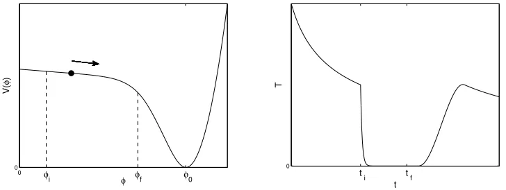
of a potential fulfilling the requirements, a Coleman-Weinberg type potential (Coleman & Weinberg 1973) is shown on the left-hand side in Fig. 1.6.

During inflation, the universe expanded by at least a factor of 1030_{. Its} constituents, i.e. radiation and particles, potentially contributing substan-tially to the energy density prior to inflation, have been extremely diluted. At the end of inflation, the temperature had dropped down to essentially zero; the universe was cold and empty except for the scalar inflaton field. Shortly afterwards, the inflaton decayed completely and all of its energy was injected into the particle sector; this epoch is called reheating (Abbott et al. 1982; Kofman et al. 1994, 1997). During reheating, the temperature increased to about its original value and the universe was repopulated with the precursors of present day particles and radiation. We qualitatively sketch the thermal history of the early universe in the right-hand panel of Fig. 1.6.

Besides from the simple model of a single scalar field as described above, the era of inflation can be realized within a variety of scenarios which only need to mimic a scalar condensate in slow-roll regime. For example, in k -inflation, an exponential expansion is achieved even without a potential term (Armend´ariz-Pic´on et al. 1999; Garriga & Mukhanov 1999). In this models, the inflaton Lagrangian Eq. 1.19 gets modified to contain higher order (i.e. non-quadratic) terms,

Lφ→Lbφ=P(φ, X), (1.29)

whereP is a functional ofX _≡gµν_∂

µφ ∂νφ. To obtain a slow variation of the

(27)

0 0

φ

V(

φ

)

φ_i φ_f φ₀

0

t

T

t_i t_f

Figure 1.6: Qualitative sketch of inflation. Left panel: The inflaton field evolves slowly from its initial false vacuum state atφi to the minimum of the

potential at φ0. Inflation ends atφf, when the kinetic energy of the inflaton

can no longer be neglected. Right panel: Prior to inflation, the temperature decreases moderately with time, T _∝ a−1 _∝ _t−1/2_{. With the onset of the} exponential expansion at ti, particles and radiation get rapidly diluted and

the universe becomes cold and empty. Aftertf, the end of inflation, reheating

increases the temperature to about its original value.

differs generically from the speed of light. In another class of models, the assumption is relaxed that the inflaton field drives both the expansion of the universe and the generation of the primordial perturbation. Motivated by particle physics, in multiple field inflationary models (Linde 1990a; Copeland et al. 1994) at least one additional scalar field χ is introduced which may couple to the inflaton via a modified potential term in the Klein-Gordon equation (Eq. 1.22),

V′(φ)_→Vb′(φ, χ). (1.30)

Likewise, by adding corrections to the Einstein-Hilbert term of the action Eq. 1.18, it is possible to realize inflation entirely within the theory of gravity (Barrow & Ottewill 1983; Starobinskiˇi 1983). With the introduction of higher order spatial curvature terms,

S →Sb=

Z

d4x√₋g

1

2R+c1R

2₊_c

2RµνRµν+. . .

(28)

the equations of motions are no longer of second order only. Thereby, the gravitational field has gained extra degrees of freedom, generically including a scalar field that can imitate the role of the inflaton.

1.4 Inflation and non-Gaussianity

1.4.1 Classification scheme

The properties of the universe after the epoch of inflation are, to a large extent, independent of the details of its actual physical realization. This, on the one hand, makes inflation a robust theory with strict and well testable predictions. On the other hand, if we would like to learn more about the underlying scenario, we are forced to develop and conduct sophisticated ex-periments. On closer inspection, it turns out that there are three general tests inflationary models can be put to: measurements of the tilt of the pri-mordial power spectrum, the test for relic gravitational waves, and the search for primordial non-Gaussianity.

If the inflaton was responsible for both driving the exponential expansion and generating the primordial perturbations, measurements of the spectral tilt and its scale dependence turn out to be a valuable tool to distinguish between various slow-roll models. A deviation from the Harrison-Zeldovich spectral index ns = 1 has been successfully proven by WMAP data (see

Table 1.1) and experiments at the sensitivity level of the Planck satellite mission will significantly constrain the functional form of the inflaton poten-tial. However, if the assumption of a single field in slow-roll approximation is relaxed, measurements of the spectral tilt may lose their predictive power to a large extent (Bartolo et al. 2004).

(29)

exacer-bate the situation. Besides from measuring effects of incident gravitational waves directly, a promising avenue towards a detection is to search for so called B-modes in the polarization signature of the CMB radiation. How-ever, for the time being, it has only been possible to impose upper limits on the strength of primordial gravitational waves (see, e.g., Jenet et al. 2006; Ade et al. 2008; The LIGO Collaboration & The Virgo Collaboration 2009; Komatsu et al. 2010).

The third test for inflationary models is the search for non-Gaussian sig-natures in the primordial perturbations. For the simplest models of inflation, linear theory predicts them to be Gaussian (Maldacena 2003; Creminelli & Zaldarriaga 2004, see also Sect. 1.4.2). Very recently, the full second order treatment of the problem has quantified the corrections to this prediction (Beneke & Fidler 2010; Pitrou et al. 2010); the effect of non-linear mode coupling introduces small non-Gaussian phase correlations. In order to real-ize this lowest possible level of non-Gaussianity, four conditions have to be fulfilled (Bartolo et al. 2004):

• Slow-roll condition. The large friction term in the Klein-Gordon equa-tion (Eq. 1.22) highly suppressed temporal variaequa-tions of the inflaton field, _|φ˙_{| ≪}1.

• Single field model. Both the accelerated expansion of the universe and the generation of the primordial perturbations were driven by a single scalar field.

• Canonical kinetic term. The kinetic term in the inflaton Lagrangian Eq. 1.19 is given by the canonical quadratic term, i.e., T _∝gµν_∂

µφ ∂ν.

• Bunch-Davies vacuum. The evolution of the inflaton field started out from the preferred de Sitter invariant ground state (Bunch & Davies 1978).

If at least one of the above mentioned conditions is violated, the primordial perturbations are no longer expected to be Gaussian. Conversely, a signifi-cant detection of non-Gaussianity in e.g. CMB radiation experiments has the potential to inevitably rule out all single field inflationary models (Creminelli & Zaldarriaga 2004).

(30)

A Gaussian random field is fully described by its power spectrum and no additional information can be extracted from the data set by calculating other statistical quantities. As for a Gaussian field then-point correlation functions vanish exactly ifn is odd, the lowest non-trivial order, the 3-point function, turns out to be a powerful tool to test an arbitrary field for a non-Gaus-sian contribution. For our particular purpose, i.e. for the analysis of CMB radiation data, it turns out to be convenient to consider the corresponding Fourier transform, the so calledbispectrum, which we defined as

hΦ(~k1)Φ(~k2)Φ(~k3)i= (2π)3δ3(~k1 +~k2+~k3)F(k1, k2, k3). (1.32)

Here, Φ is the gauge invariant metric perturbation as introduced by Bardeen (1980), and F(k1, k2, k3) defines the shape function which fully character-izes the momentum dependence of the specific bispectrum signature (Babich et al. 2004; Fergusson & Shellard 2009). Restricted to sub-horizon scales and written in longitudinal (conformal-Newtonian) gauge, the perturbations Φ coincide with the ordinary Newtonian gravitational potential up to a minus sign (Mukhanov 2005).

Dependent on the process responsible for the generation of primordial non-Gaussianity, the function F(k1, k2, k3) in Eq. 1.32 will take different shapes. As a result, it is possible to characterize the functional dependence of the bispectrum in terms of the contribution from different momentum vec-tors according to the underlying physical model responsible for generating the non-Gaussianity. For example, we obtain

Fequ(k1, k2, k3)∝

(k1+k2−k3)(k2+k3−k1)(k3+k1−k2) k1k2k3

(1.33)

for non-Gaussianity of equilateral type, as predicted by inflationary models with modified kinetic term in the inflaton Lagrangian (Babich et al. 2004). Here, a considerable amount of power comes from momentum configurations where k1 ≈ k2 ≈ k3, i.e. from modes that were shifted outside the horizon during inflation at roughly the same time.

(31)

highest energies, it is nevertheless possible to predict the expected contribu-tion to the bispectrum,

Fvac(k1, k2, k3)∝ 1

k3 1k32

+ 1

k3 1k33

+ 1

k3 2k33

+ 3

k2

1k22k32 − 1

k1k22k23 − 1

k1k32k22

− 1

k2k21k32

− 1

k2k23k21

− 1

k3k12k22

− 1

k3k22k21

. (1.34)

Here, the most important configuration of the momenta in the shape function is approximately given by kh ≈ki ≈kj/2 (Chen et al. 2007).

Likewise, if we violate the single field condition, we introduce non-Gaus-sianity of local type,

Floc₍_k

1, k2, k3)∝ 1

k3 1k23

+ 1

k3 1k33

+ 1

k3 2k33

=

P

iki3

Q

iki3

, (1.35)

where most of the power stems from modes which satisfy the squeezed trian-gle configuration, kh ≈ki ≫kj (Babich et al. 2004). The shape functions of

the three inflationary classes discussed are plotted in Fig. 1.7. As they are intrinsically very different, it will be possible to discern between them once a significant detection of non-Gaussianity has been made.

We will concentrate on local non-Gaussianity in the remainder of the thesis. It has been proven to be of particular importance, as a significant detection of that kind of non-Gaussianity would inevitably rule out all sin-gle field inflationary models (Creminelli & Zaldarriaga 2004), irrespective of other details of their realization (e.g. form of the inflaton potential, ground state, kinetic term, or slow-roll condition). The shape function Eq. 1.35 of non-Gaussianity of local type was derived from the characteristic functional form of the primordial perturbations Φ. When perturbatively expanded in the regime of weak non-Gaussianity, multi-field inflationary models predict a specific non-Gaussian signature which is localized in real space (Salopek & Bond 1990; Gangui et al. 1994),

Φ(r) = ΦL(r) +fNL ΦL2(r)− hΦ2L(r)i

. (1.36)

(32)

(33)

limits on the amplitude of non-Gaussianity from the WMAP 7-year data release are

−10< fNL <74

at 2-σ level (Komatsu et al. 2010). This result was derived within a fre-quentist approach by means of a bispectrum estimator (Komatsu et al. 2005; Smith et al. 2009). In the limit of vanishing non-Gaussianity, the estimator is optimal, i.e. it saturates the Cramer-Rao bound.

The data obtained with the Planck satellite mission will allow for a sig-nificant improvement of the error bars by almost one order of magnitude—a Fisher matrix forecast predicts a formal 1-σ error in fNL of about 5 for a CMB radiation temperature only analysis which may be further improved to finally achieve a fNL of 3 if polarization information is taken into account (Yadav et al. 2007).

1.4.2 Single field inflation

For simple inflationary models where only one dynamical field was present, the level of primordial non-Gaussianity from first order perturbation theory is predicted to be very small (Gangui et al. 1994; Maldacena 2003; Creminelli & Zaldarriaga 2004; Lyth 2007; Bartolo et al. 2008). To relate to this result, we follow the arguments in Creminelli & Zaldarriaga (2004) and first define the curvature perturbations1_,_ζ_{, via the spatial components of the metric of} uniform energy density slices,

gij ≡a(t)2e2ζ(t,x)hij(t, x), (1.37)

where hij encodes the tensor perturbations, but will be of no relevance for

our discussion here, i.e. it is save to assume hij =δij.

Interested in the bispectrum ofζ in the squeezed limit, we set k1 ≪k2, k3 without loss of generality and write

hζ(~k1)ζ(~k2)ζ(~k3)i ≈ hζ(~k1)hζ(~k2)ζ(~k3)i_ζ₍_~k₁₎i, (1.38) where the 2-point function _hζ(~k2)ζ(~k3)i is to be evaluated for a given value ζ(~k1).

1

Note, that in the matter dominated era, the curvature perturbations can simply be rewritten in terms of the gauge invariant potential, Φ = 3

(34)

In the relevant regime, i.e. when the modes k2 and k3 are crossing the horizon, k1 is already far outside the horizon and therefore frozen (Salopek & Bond 1990). As a result, it is justified to consider ζ(~k1) =ζB as a purely classical background affecting the metric Eq. 1.37 only on the largest scales. We now consider the real space expression of _hζ(~k2)ζ(~k3)iζB, and expand

it to linear order for small perturbations of the background,

hζ(~x2)ζ(~x3)iζB =hζ(~x₂)ζ(~x₃)i_ζB₌₀+ζB

∂

∂ζBhζ(~x2)ζ(~x3)iζB

ζB₌₀+O((ζ

B₎2₎_.

(1.39) As the wave vector k1 is small with respect to k2 and k3, we first note that the background ζB _{is almost constant over the relevant distances} _~x

2 −~x3. As a result, the small-scale dependency of_hζ(~x2)ζ(~x3)iζB must be attributed

solely to the change of the physical distance as mediated by the metric,

δxphys =aeζ

B

δx. Therefore, it is possible to rewrite the derivative in Eq. 1.39,

∂

∂ζBhζ(x)ζ(0)iζB=x d

dxhζ(x)ζ(0)iζB. (1.40)

Substituting this expression into Eq. 1.39 will lead after a Fourier transfor-mation to the consistency relation (Maldacena 2003)

lim

~k1→0

hζ(~k1)ζ(~k2)ζ(~k3)i ≈(2π)3δ(~k1+~k2+~k3) (1−ns)P(k1)P(k2), (1.41) where we made use of the primordial power spectrum _P(k) and its spectral tilt according to 1₋ns ≡ −dln(k

3_P₍_k₎₎

dlnk . As the spectral tilt is known to be

small, the primordial non-Gaussianity of local type in single field inflationary models is vanishing, fNL <1.

For the calculation presented here, no assumptions on the specific model were made, thus, the result is valid for single field inflation in general. How-ever, in this simple approach, one relies on a strictly classical prescription of the process neglecting quantum mechanical effects. Once the calculation is repeated within a proper field theoretical framework, the above conclusion may not hold in full generality (Ganc & Komatsu 2010).

1.4.3 Generating primordial non-Gaussianity

(35)

a crucial role in the process of generating the primordial perturbations. A simple and well studied model falling within this important class is the curva-ton scenario (Mollerach 1990; Linde & Mukhanov 1997; Moroi & Takahashi 2001; Enqvist & Sloth 2002; Lyth & Wands 2002).

Here, a weakly coupled second scalar field is introduced, the curvaton

χ, which has a small mass during inflation but contributes negligibly to the total energy density. Therefore, its quantum fluctuations initially sources perturbations of isocurvature (entropy) type. After the end of inflation, when the inflaton has already decayed into radiation, the temperature of the universe drops such that the curvaton field’s energy density eventually contributes an important fraction to the total energy density. In this epoch, it becomes a source of curvature fluctuations. It starts to oscillate around the minimum in an approximately quadratic potential. As the curvaton obeys the equation of state of a cold, non-relativistic fluid with equation of state parameter w = 0, its energy density decreases as ρχ ∝ a−3 and therefore

more slowly than that of the radiation (scaling asργ ∝a−4). In order not to

dominate the total energy density at later times, the curvaton is supposed to decay well before the onset of primordial nucleosynthesis. During decay into thermalized radiation, the inhomogeneous density of the curvaton field will finally be converted into primordial adiabatic perturbations.

Besides from generating primordial perturbations after the end of infla-tion, another important difference to the conventional single field model is the fact that the seed fluctuations originally are of isocurvature instead of adiabatic type. As a result, the mechanism responsible for suppressing non-Gaussianity in the single field models is no longer valid. For a more quantita-tive description of the underlying processes in multi-field models in general, we shall review the so called δN formalism in the following (Starobinskiˇi 1985; Salopek & Bond 1990; Sasaki & Stewart 1996; Lyth et al. 2005; Lyth & Rodr´ıguez 2005).

We start out from the definition equation of the curvature perturbation Eq. 1.37. Written in this way, ζ can be interpreted as the perturbation to the scale factor lna(t). Allowing for a spatially inhomogeneous expansion factor, N(t)_→N(t, x), we find that the curvature perturbation encodes the fluctuations in the expansion,

ζ(t, x) =δN

(36)

where we introduced the unperturbed median expansion rate _hN(t, x)_ix ≡

ln_aa₍(_tt)

i). As a rough estimate, one can obtain ζ from the spatial variations in

the duration of the expansion,

ζ _≈H δt

≈Hδχ

˙

χ , (1.43)

whereχis the relevant scalar field, e.g. the inflaton, or the curvaton. Finally, we assume that the dynamical evolution of each patch of the universe is independent of all other patches (‘separate universe’ assumption). With this simplification, the energy is locally conserved (Rigopoulos & Shellard 2003; Lyth et al. 2005).

Given an arbitrary number of light scalar fields with small Gaussian fluc-tuations, χi(x) = ¯χi+δχi(x), we derive an approximate expression for the

small inhomogeneities in the expansion factor,

δN _≈N,iδχi+ 1/2N,ijδχiδχj +O(δχ3), (1.44)

where we defined the partial derivative of N via N,i ≡ ∂N_∂χ_i, and sum over all

repeated indices. We identify the nearly flat power spectrum of the scalar field perturbations (Bunch & Davies 1978),

hδχ(k1)δχ∗(k2)i= (2π)3 H2

_ 2k3 1

δ(k1−k2), (1.45) where we used the Hubble parameter at horizon exit of the corresponding modes,H_. Combining Eq. 1.42 and Eq. 1.44, we conclude for the curvature perturbation power spectrum at first order (Sasaki & Stewart 1996)

hζ(k1)ζ∗(k2)i= (2π)5 Pζ 2k3

1

δ(k1−k2), (1.46)

where

Pζ =

H_ 2π 2_X i N2

,i. (1.47)

In analogy to Eq. 1.36, we introduce the level of non-Gaussianity, fNL, as overall prefactor to a non-linear transform of the curvature perturbations,

ζ(r) =ζL(r) + 3

5fNL ζ 2

L(r)− hζL2(r)i

≡ζL(r) + 3

(37)

Interested in the corresponding expression in momentum space, we rephrase the non-Gaussian term as

ζN L(k) =

Z

d3_p

(2π)3ζL(k+p)ζ

∗

L(p)−(2π)3σ2δ3(k), (1.49) where the second term subtracts the varianceσ2_{of the field to ensure}_h_ζ

N Li=

0. Now, we identify an important non-vanishing contribution to the bispec-trum (Komatsu & Spergel 2001),

hζ(k1)ζ(k2)ζ(k3)i ⊇ hζL(k1)ζL(k2)ζNL(k3)i+ 2 cycl. = 6

5fNL(2π) 3_[_P₍_k

1)P(k2) + 2 cycl.] . (1.50)

On the other hand, we use Eq. 1.44 to expand the expression to fourth order in δχ,

hζ(k1)ζ(k2)ζ(k3)i=N,iN,jN,hhδχi(k1)δχj(k2)δχh(k3)i

+N,iN,jN,hk[hδχi(k1)δχj(k2)δχh(k3)δχk(k3)i+ 2 cycl.]

+_O(δχ4). (1.51)

The first term on the right hand side vanishes as it contains the expectation value of an odd number of independent Gaussian variables. For an explicit expression of the amplitude of non-Gaussianity, we finally obtain (Lyth & Rodr´ıguez 2005; Byrnes et al. 2006; Sasaki et al. 2006)

fNL = 5 6

P

ijN,ijN,iN,j

(P_iN2

,i)2

, (1.52)

where we have used Eq. 1.45 and Eq. 1.47 to rewrite H_ in terms of deriva-tives of N.

An application of this formula to the curvaton scenario as discussed above allows us to predict the range of non-Gaussianity expected in this model. Considering perturbations in the curvaton field around a mean value ¯χ, χ=

¯

χ +δχ, we find for the contribution to the energy density in a quadratic potential (Tseliakhovich et al. 2010)

¯

ρχ ∝ hχ2i

= ¯χ2 +_hδχ2_i, hence

δρχ ¯ ρχ ≈ 2δχ ¯ χ +

δχ2_{− h}_δχ2_i ¯

(38)

Obviously, the above equation resembles the definition equation of local non-Gaussianity, Eq. 1.36. Any non-Gaussian signature in δρχ will finally be

imprinted onto the CMB radiation.

We now define N as expansion factor from the onset of the oscillations of the curvaton field after the end of inflation until its decay. We introduce the ratio of the curvaton energy density compared to the total energy density at decay timetf,

r= ρ

χ f

ρf

. (1.54)

In the following, we focus on the most relevant case, the limit of a radiation dominated universe, r <1.

For a slice of uniform total energy density, the perturbation of the expan-sion factor is given by

δN =rδρ

χ f

4ρχ_f , thus (1.55)

N =rln(ρ

χ f)

4 +C1, (1.56)

where we introduced an arbitrary constant of integration. We now make use of the fact that the curvaton energy density perturbation remains con-stant during the period considered here, and rewrite it as a function of the amplitude of the curvaton field when the oscillation started,χi,

N =rln(1/2m 2

χχ2i)

4 +C1

=rln(χi)

2 +C2, (1.57)

where we have used a quadratic approximation for the potential V(χ), and the particle mass mχ. Finally, we apply Eq. 1.52 to predict the level of

non-Gaussianity of local type in the curvaton scenario,

fNL = 5 6

N,χχ

(N,χ)2

=₋ 3

5r. (1.58)

(39)

bounds (Komatsu et al. 2010). The analysis can be extended to the case of two or more curvaton fields (Assadullahi et al. 2007; Choi & Gong 2007), or to include higher order terms in the curvaton potential, leading to a non-linear dynamical evolution prior to the decay (Enqvist & Nurmi 2005; Huang 2008). As a result, the predicted value of fNL can also become large and positive (Enqvist et al. 2010).

We now review another class of early universe scenarios predicting a sig-nificant level of local non-Gaussianity. The ekpyrotic and cyclic universe models were recently introduced to apply concepts adopted from string the-ory within a cosmological framework (Gordon et al. 2001; Khoury et al. 2001, 2002; Notari & Riotto 2002; Steinhardt & Turok 2002a,b). Although not yet fully understood and still plagued by very serious problems (see, e.g., Kallosh et al. 2001; Lyth 2002; Kallosh et al. 2008; Linde et al. 2010, especially violat-ing the null energy condition turns out to be problematic), these models may offer a way to overcome some shortfallings of inflation. Here, the period of in-flation gets completely replaced by a phase of slow contraction postulated to take place prior to the big bang. It can be shown that during such an epoch, almost scale-invariant scalar perturbations in a flattened region of space can be generated, resolving the problems of standard cosmology (Erickson et al. 2007). In addition to the absence of gravitational waves, a significant level of local non-Gaussianity is predicted, both potentially observational signa-tures that in principle would allow to distinguish ekpyrotic models from the simplest inflationary scenarios.

To realize an ekpyrotic epoch of contraction, we first note that from Eq. 1.9 we can derive the general functional dependence of the energy density of a particle species on the scale factor,

ρ _∝a−3(1+w). (1.59)

In the pre-bounce contracting phase, the existence of a component with a very large equation of state parameter w_≫1 is postulated. Once the scale factor decreases, it will finally dominate over matter (ρm ∝ a−3) and radiation

(ργ ∝ a−4). As a result, the relative energy density of radiation and its

perturbations will decrease until it eventually becomes a negligible fraction of the total energy density; the space becomes flat.

(40)

is necessary (Koyama & Wands 2007; Koyama et al. 2007b). For simplicity, however, we will restrict the discussion to single field ekpyrotic models in the following.

For the self-interaction of the scalar field, a steep, negative potential is required in ekpyrotic scenarios, e.g. of the form (Buchbinder et al. 2007; Lehners et al. 2007)

V(χ) =₋V0e−Cχ, (1.60)

where C is a positive constant. This is a simple parametrization of the po-tential encountered in heterotic M-theory (Hoˇrava & Witten 1996; Witten 1996; Lukas et al. 1999b,a). The original version of ekpyrotic models pro-posed an effective 5-dimensional Universe consisting of two bounding (3+1)-dimensional branes separated through a finite bulk volume. The visible of the two branes corresponds to the usual four-dimensional universe we live in, whereas the hidden brane remains inaccessible (Khoury et al. 2001). Then, the potential Eq. 1.60 induces a force acting along the fifth dimension with a certain probability to make the branes collide. Such an approach, collision, and subsequent phase of recession corresponds to a full cycle in the evolution of the universe with collapse, bounce, and expansion. Here, we will assume a regular bounce during which the curvature perturbations on super-horizon scales remain unaffected. As a result, the entropy perturbations generated during the ekpyrotic phase can be directly mapped to the adiabatic pertur-bations after the bounce.

Following Koyama et al. (2007a); Creminelli & Senatore (2007); Lehn-ers (2010), to quantify the non-Gaussian contribution expected in ekpyrotic models, we neglect the effect of gravity. We consider small perturbations of the scalar field χ around its mean value, χ(x, t) = ¯χ(t) +δχ(x, t), and start out with the evolution equation of the unperturbed spatially invariant field,

¨

χ(t) +V,χ(χ(t)) = 0, (1.61)

and constrain the functional form of the potential by requiring a scale in-variant power spectrum of the field perturbations. For the Fourier modes of the fluctuations, the equation of motion takes the form of a wave equation (Creminelli & Senatore 2007),

¨

δχ+k2₊_V

,χχ(χ)

δχ = 0. (1.62)

In the regime V,χχ <−k2 <0, the solution to Eq. 1.62 stops oscillating and

(41)

obtain a power law solution in this region of parameter space. Adopting this form, one finds the asymptotic behavior of the field perturbations,

δχ(k, t)_∝k−1/2f(kt), (1.63) where the function f(kt) describes the oscillatory behavior of the pertur-bations. To maintain a scale invariant solution after freeze-out, we enforce

δχ(k, t) _∝ t−1 _{and eventually obtain the explicit expression for the second} derivative of the potential

V,χχ =−

2

t2 . (1.64)

Finally, we find the normalized solution to Eq. 1.62,

δχ(k, t) = √1

2k

1₋ i

kt

e−ikt. (1.65)

To derive an explicit expression for the potential, we calculate the time derivative of Eq. 1.61,

...

χ ₋ 2

t2χ˙ = 0, (1.66)

with power law solution ˙χ(t) = ₋2M/t, where we introduced a constant of integration M and neglected the decaying term _∝ t2_{. Integration yields to} the expression

χ(t) =₋2Mlog(₋t) +_C, (1.67)

which we use to replace the time variable in the equation for the potential

V,χχ =−2/t2 in favor of χto finally obtain

V(χ) =₋V0eχ/M, (1.68)

resembling the suggested functional form of the potential in Eq. 1.60. To calculate the level of non-Gaussianity in ekpyrotic models, we adopt the procedure of Maldacena (2003) and write the leading order component in the bispectrum by means of the interaction Hamiltonian,

hδχ(k1)δχ(k2)δχ(k3)i=−i

Z t

−∞h

δχ(k1)δχ(k2)δχ(k3)Hint(t′)idt′+ c.c.,

(42)

The cubic self-interaction is described by

Hint(t) =

V,χχχ

3! δχ 3

=₋2

t2 δχ3

3!M , (1.70)

where we made use of Eq. 1.68. Substituting Eq. 1.65, it is possible to identify the leading order term in the bispectrum for small t (Creminelli & Senatore 2007),

hδχ(k1)δχ(k2)δχ(k3)i= (2π)3δ(k1+k2+k3)

P

iki

Q

iki

1

8Mt4 . (1.71)

The characteristic momentum dependence found here unravels a non-Gaus-sian contribution of local type (cf. Eq. 1.35).

The free choice of the parameter M results in a model dependent non-Gaussian contribution. However, in reasonable scenarios, the expected range of non-Gaussianity lies around ₋50 . fNL . 60 (Lehners & Renaux-Petel 2009)—it is significantly wider than for single field inflationary models.

1.4.4 Secondary sources of non-Gaussianity

Due to a tight coupling between the primordial plasma and photons, non-Gaussianity in the perturbations will leave an imprint onto the CMB ra-diation, opening up the opportunity to construct dedicated tests searching for this signature. However, as various physical mechanisms are capable of modifying the pristine fluctuations in the CMB radiation on their way from recombination at redshift z _≈ 1100 to the detectors at present time (Aghanim et al. 2008), secondary non-Gaussianity of non-primordial origin will be induced. As it is imperative to quantify the expected amount of contamination, these effects have been subject to extensive studies in liter-ature (e.g. by Goldberg & Spergel 1999; Spergel & Goldberg 1999; Verde & Spergel 2002; Castro 2003; Serra & Cooray 2008; Hanson et al. 2009; Khatri & Wandelt 2009; Pitrou 2009).

The most important among all possible contributions to non-primordial non-Gaussianity stems from the correlation between the non-linear integrated Sachs-Wolfe effect2 _{(ISW, Sachs & Wolfe 1967) and weak gravitational} lens-ing. The ISW effect, originating from the time evolution of the gravitational

2

(43)

potential during photon crossing, affects the CMB radiation pattern on large scales. Contrary, lensing induced by galaxy clusters (themselves residing in potential wells), modifies the fluctuations on small scales. The correlation between these two effects will, therefore, peak for squeezed triangle momen-tum configurations, mimicking the shape function of non-Gaussianity of local type. While for WMAP data this mechanism should lead to only a small bias ∆fNL ≈3 (Komatsu et al. 2010) which has not been detected directly (Mun-shi et al. 2009), for the analysis of Planck satellite data the effect will play an important role and may lead to a contribution of up to ∆fNL ≈10 (Mangilli & Verde 2009).

Beyond, radiation from residual point sources has been discussed as pos-sible secondary source of non-Gaussianity. They are either radio sources, lu-minous infrared galaxies, or galaxy clusters inducing spectral distortions due to Compton upscattering of CMB photons via the Sunyaev-Zeldovich effect (Sunyaev & Zeldovich 1970). To reasonable approximation, they have a con-stant bispectrum amplitude which is independent of the multipole moments considered, though their contribution varies in different frequency bands (Ko-matsu et al. 2003). To reduce the effect of radio sources, a point-source mask is usually imposed to the data prior to the analysis, constructed either from the CMB radiation maps themselves, or with the help of dedicated radio surveys as e.g. the GB6 (Gregory et al. 1996), or the PMN surveys (Griffith & Wright 1993). However, as sources can only be detected and removed down to an experiment-specific flux limit, a residual contribution will remain in the data. Recently, an estimate of the contribution of point sources to local non-Gaussianity has been quantitatively specified. The correction is most important at low frequencies but will probably not exceed ∆fNL . 1 for Planck data (Babich & Pierpaoli 2008).

(44)

template, Haslam et al. 1981), Hα line emission maps (free-free template, Finkbeiner 2003), and infrared emission data (dust template, Finkbeiner et al. 1999). To constrain the foreground emission at the frequencies of the CMB radiation experiment, the templates have to be extrapolated assuming a specific spectral index for the component. A comparison between the de-ducedfNL values from raw and cleaned WMAP 7-year data indicates that the smooth components amount for a non-Gaussian signal of about ∆fNL ≈ 10 when a conservative sky mask is imposed (Komatsu et al. 2010). However, the residuals after template marginalization are probably negligible (Smith et al. 2009).

The issue of a different kind of non-Gaussianity, primary non-Gaussianity, has recently been comprehensively addressed in Pitrou et al. (2010) (see also Beneke & Fidler 2010). It specifies the contribution from phase correla-tions arising due to non-linear processes between the end of inflation and recombination. To quantify this contribution, the full second order Boltz-mann equation was solved, including all components of the cosmic fluid. It was found that these effects will induce excess non-Gaussianity at a level of about ∆fNL ≃5.

1.5 Bayesian statistics

In this thesis, we pursue the goal to develop a Bayesian method to search for non-Gaussianity in CMB radiation data. Unfortunately, using Bayesian statistics is still a less common alternative to the currently predominant fre-quentist approach—we therefore briefly outline its foundations in what fol-lows (for a more comprehensive discussion, see the textbooks of, e.g., Leonard & Hsu 2001; Gill 2002; MacKay 2005; Bolstad 2007; Hobson et al. 2010).

The frequentist approach is characterized by basic ideas that can be sum-marized as follows:

• Probabilities are defined as relative frequencies in infinite repetitions of random experiments.

• The parameters that characterize a population are fully determined yet unknown constants.

(45)

In the frequentist approach, it is only possible to quantify the proba-bility of random variables. But as physical parameters like e.g. the speed of light, Newton’s constant, or the level of primordial non-Gaussianity are fixed, probability statements about their numerical values cannot be made. To cir-cumvent this problem, a sampling distribution is constructed, the probability distribution of a given statistic obtained from random samples drawn from the population. Finally, a confidence interval of the parameter is deduced from the width of that distribution.

An intrinsic shortcoming of this procedure is the ambiguity in the def-inition of estimators, i.e. the statistics used to measure the parameter of interest. For a given problem, several of them can usually be constructed. In general, their outcome will be different, necessitating the development of so-phisticated methods to judge over performance and reliability of estimators. Another objection concerns the generation of the sampling distribution. As it involves random realizations drawn from the population that actually have not been observed in the experiment, information other than that carried in the data become relevant.

Bayesian statistics, on the contrary, is based on an extended interpreta-tion of probability. Here, it is used in a more general way, to measure a

degree of belief in a certain proposition. On the basis of three axioms, it is possible to map the degree of belief onto a probability (Cox 1946). Denoting the degree of belief in proposition aby D(a), we define the degree of belief in a conditional propositionagiven a second propositionb to be true byD(a_|b). Then, the axioms are:

• Ordering: If D(a)_≤D(b) and D(b)_≤D(c), thenD(a)_≤D(c), where “_≤” is a suitable order operator.

• Negation: There exists a relation f between the degree of belief in a proposition a and its negation ¯asuch that D(a) = f[D(¯a)].

• Conjunction: A conjunction of propositions a and b can be expressed via a function g such that D(a, b) = g[D(a_|b), D(b)], where D(a_|b) is the conditional degree of belief as defined above.

If the axioms are fulfilled, the degrees of belief can be mapped onto usual probabilities with the well-known properties, P(false) = 0, P(true) = 1, 0 _≤ P(a) _≤ 1, and comply with the relations P(a) = 1₋P(¯a), P(a, b) =

(46)

With this redefinition, we can apply the concept of probability to a much broader class of problems from the outset. For example, although the Hubble constant is not a random variable, we may ask the question: “What is the probability to find its current value within the range 69km s−1_Mpc−1 _≤ H0 ≤ 71km s−1Mpc−1?” It is important to note that we are forced to provide limits like that toH0 because our knowledge about its true value is incomplete, not because it is the outcome of a random experiment with a given probability distribution.

The cornerstone of Bayesian statistics is the theorem of Bayes that allows to specify how the knowledge about a parameter of interest λ should be updated after new data D were taken into account (Bayes & Price 1763). It formally results from symmetry considerations of the joint distribution of two events; from

P(λ, D) =P(λ_|D)P(D), and

P(λ, D) =P(D, λ)

=P(D_|λ)P(λ), we follow

P(λ_|D) = P(D|λ)P(λ)

P(D) . (1.72)

In the above expression, P(λ) is the prior distribution, representing our knowledge aboutλbefore the data were taken into account,P(D_|λ) is the so called likelihood function of the parameter, and the normalization constant

P(D) is the evidence. Together, they build up the posterior distribution,

P(λ_|D), which mirrors our updated knowledge about the parameter after the data have been analyzed.

Let us now summarize the main characteristics of the Bayesian approach to statistics:

• The parameters we want to constrain are put on the same level with random variables.

• We use the degree of belief to interpret probability statements about parameters.

• Inference about parameters is made by directly applying the rules of probability calculus.

(47)

Contrary to the frequentist approach, the Bayesian concept offers a con-sistent and unambiguous way to update our (subjective) prior knowledge about a parameter when new data become available. That is, an indepen-dent analysis that makes use of the same data and prior distribution will lead to identical results. Furthermore, only information from the data that have actually been observed enter the analysis, obviating the necessity to construct sampling distributions from possible (but unrealized) outcomes of the experiment.

For illustrative purposes, we include a brief discussion of a simple example (based on MacKay 2005) to compare the two schools of statistics against each other. Let us assume that a coin have been tossed N = 250 times and a sequence of nh = 141 heads was observed. Now, we want to contrast the

hypothesis _H0 “the coin is fair” with hypothesis H1 “the coin is biased” in a quantitative way.

In the frequentist analysis, which we discuss first, one completely concen-trates on the null hypothesis. We expect the number of heads to follow a binomial distribution

P(nh|N, p) =

N nh

pnh₍₁₋_p₎N−nh_, _(1.73)

wherep_≡1/2 for a fair coin as stated in_H0. Then, we specify the probability to find an as extreme value for nh as observed in the data,

P(nh= 141) = 2

250

X

n=141

250

n

1/2250

= 0.0497, (1.74)

i.e. in the frequentist analysis, we reject the null hypothesis at a significance level of 5 %. As a result, we conclude that the coin is biased at a confidence level of 95 %.

We will now focus on the Bayesian analysis. In the language of Bayesian statistics, we have to perform a model comparison between model _H0 (the coin is fair) and model _H1 (the coin is biased) given the data. To this end, we define the probabilities of (that is, our degree of belief in) _H0,

P(_H0|nh) =

P(nh|H0)P(H0) P(nh)

(48)

and _H1,

P(_H1|nh) =

P(nh|H1)P(H1) P(nh)

, (1.76)

using Bayes’ theorem. For the analysis, we further have to specify the sub-jective prior distribution ofp which we choose to be flat, P(p_|H1) = 1. Not preferring any of the two hypotheses a priori (i.e.P(_H0)≡P(H1) = 1/2), we construct the so called Bayes factor, the likelihood ratio of the hypotheses,

P(nh|H1) P(nh|H0)

=

R1 0 dp p

nh(1−p)N−nhP(p|H 1) (1/2)nh(1−1/2)N−nh

=

141!109! 251! (1/2)250

= 0.61. (1.77)

In fact, the Bayesian analysis reveals that hypothesis _H0 is actually slightly

preferred over hypothesis _H1, i.e. for the choice of the prior as stated above, we conclude that the coin is fair. Note, however, that a Bayes factor close to one signalize indecisive data. The result will therefore be relatively sensitive to the prior distribution P(p_|H1). But even for an overidealized choice of the prior—an a posteriori constructed delta function exactly matching the relative frequency of heads in the data,P(p_|H′

1) =δ(p−141/250)—we obtain a Bayes factor of

P(nh|H′1) P(nh|H0)

= p

141₍₁₋_p₎109

p=141₂₅₀ (1/2)250

= 7.8, (1.78)

indicating only moderate evidence in favor of _H′

1.

(49)

1.6 Outline of the thesis

(50)

(51)

Chapter 2 Improved simulation of

non-Gaussian temperature and

polarization CMB maps

Franz Elsner1_{, and Benjamin D. Wandelt}2,3,4

Originally published in Astrophysical Journal Supplement, 2009, 184, 264

1

Max-Planck-Institut f¨ur Astrophysik, Karl-Schwarzschild-Straße 1, 85748 Garching, Germany

2

Department of Physics, University of Illinois at Urbana-Champaign, 1110 W. Green Street, Urbana, IL 61801, USA

3

Department of Astronomy, University of Illinois at Urbana-Champaign, 1002 W. Green Street, Urbana, IL 61801, USA

4

(52)

Abstract

We describe an algorithm to generate temperature and polarization maps of the cosmic microwave background radiation containing non–Gaussianity of arbitrary local type. We apply an optimized quadrature scheme that allows us to predict and control integration accuracy, speed up the calculations, and reduce memory consumption by an order of magnitude. We generate 1000 non–Gaussian CMB temperature and polarization maps up to a multipole moment of ℓmax = 1024. We validate the method and code using the power

spectrum and the fast cubic (bispectrum) estimator and find consistent re-sults. The simulations are provided to the community1_.

1

Elsner, Franz (2010): Search for non-Gaussian Signatures in the Cosmic Microwave Background Radiation. Dissertation, LMU München: Fakultät für Physik

Search for non-Gaussian

Signatures in the Cosmic

Microwave Background

Radiation

Dissertation

Fakult¨at f¨

ur Physik

Ludwig-Maximilians-Universit¨at M¨

unchen

vorgelegt von

Franz Elsner

aus M¨

unchen

Zusammenfassung

Abstract

Contents

Chapter 1

Introduction

1.1

A cosmic review

1.2

Standard cosmology

1.2.1

Overview

1.2.2

Problems of standard cosmology

a

ρ

(a) /

ρ

ρ

ρ

ρ

1.3

Inflation

1.3.1

The foundations of inflation

1.3.2

A simple inflationary model

1.4

Inflation and non-Gaussianity

1.4.1

Classification scheme

1.4.2

Single field inflation

1.4.3

Generating primordial non-Gaussianity

1.4.4

Secondary sources of non-Gaussianity

1.5

Bayesian statistics

1.6

Outline of the thesis

Chapter 2

Improved simulation of

non-Gaussian temperature and

polarization CMB maps