Translucent Voices: Creating Sound Pedagogy And Safe Spaces For Transgender Singers In The Choral Rehearsal

(1)

University of South Carolina

Scholar Commons

Theses and Dissertations

Fall 2018

Exploring Machine Learning Techniques To

Improve Peptide Identification

Fawad Kirmani

Follow this and additional works at:https://scholarcommons.sc.edu/etd Part of theComputer Engineering Commons

This Open Access Dissertation is brought to you by Scholar Commons. It has been accepted for inclusion in Theses and Dissertations by an authorized administrator of Scholar Commons. For more information, please contactdillarda@mailbox.sc.edu.

Recommended Citation

Kirmani, F.(2018).Exploring Machine Learning Techniques To Improve Peptide Identification.(Doctoral dissertation). Retrieved from

(2)

Exploring Machine Learning Techniques To Improve Peptide Identification

by

Fawad Kirmani

Bachelor of Technology

Chandra Shekhar Azad University of Agriculture and Technology, Kanpur, 2010

Submitted in Partial Fulfillment of the Requirements

for the Degree of Master of Science in

Computer Science and Engineering

College of Engineering and Computing

University of South Carolina

2018

Accepted by:

John Rose, Director of Thesis

Marco Valtorta, Reader

Jijun Tang, Reader

(3)

c

Copyright by Fawad Kirmani, 2018

(4)

Dedication

(5)

Acknowledgments

I would like to express my appreciation for Prof. Dr. John Rose, who as my thesis

advisor introduced me to the world of proteomics. He was a constant source of

guidance, good ideas and encouragement while working on this thesis. He has always

been patient with my questions and without his help and knowledge this thesis would

not have been completed.

I would like to appreciate all the help that I got from my lab mate Jeremy Lane,

who has helped me a lot in data preparation for my experiments. He used to dig

deep for the source of the datasets we come across while preparing one more dataset

for my experiments.

I would also like to thank Prof. Dr. Marco Valtorta and Prof. Dr. Jijun Tang for

agreeing to be part of my thesis committee. They were always ready to spare some

time from their busy schedule to answer my queries.

I would also like thank my family and friends who have been source of

(6)

Abstract

The goal of this work is to improve proteotypic peptide prediction with lower

pro-cessing time and better efficiency. Proteotypic peptides are the peptides in protein

sequence that can be confidently observed by mass-spectrometry based proteomics.

One of the widely used method for identifying peptides is tandem mass spectrometry

(MS/MS). The peptides that need to be identified are compared with the accurate

mass and elution time (AMT) tag database. The AMT tag database helps in reducing

the processing time and increases the accuracy of the identified peptides. Prediction

of proteotypic peptides has seen a rapid improvement in recent years for AMT studies

for peptides using amino acid properties like charge, code, solubility and hydropathy.

We describe the improved version of a support vector machine (SVM) classifier

that has achieved similar classification sensitivity, specificity and AUC on Yersinia

Pestis, Saccharomyces cerevisiae and Bacillus subtilis str. 168 datasets as was

de-scribed by Web-Robertson et al. [15] and Ahmed Alqurri [11]. The improved version

of the SVM classifier uses the C++ SVM library instead of the MATLAB built in

li-brary. We describe how we achieved these similar results with much lesser processing

time.

Furthermore, we tested four machine learning classifiers on Yersinia Pestis,

Sac-charomyces cerevisiae and Bacillus subtilis str. 168 data. We performed feature

selection from scratch, using four different algorithms to achieve better results from

the different machine learning algorithms. Some of these classifiers gave similar or

better results than the SVM classifiers with fewer features. We describe the results

(7)

Preface

This MS thesis is written as completion of my research work at the University of South

Carolina. I started to work on this project one year ago with Prof. Dr. John Rose

with great enthusiasm. I took this project to learn how to apply different machine

learning techniques to a given problem. By working on this project I was introduced

to the world of proteomics. I learned about identification of peptides and how it helps

in identification of proteins.

In Chapter 2, I describe the data preparation methodology to prepare the

proteo-typic and non-proteoproteo-typic dataset. I have used the datasets available at National

Cen-ter for Biotechnology Information, MassIVE (University of California at San Diego)

and Global Proteome Machine Database (GPMDB) to prepare our dataset. In data

preparation, I appreciate all the help I got from Jeremy Lane.

In Chapter 3, I have improved on the support vector classifier (SVM) described

by Ahmed Alqurri [11] and Web Robertson et al. [15]. In Chapter 4, I performed

different feature selection algorithms from scratch without considering much of

pre-vious work. In Chapter 5, I have implemented different machine learning classifiers

using feature sets from Chapter 4. In Chapter 3, 4, and 5, I have usedYersinia Pestis

and Saccharomyces cerevisiae datasets to perform machine learning algorithms. In

Chapter 6, I have improved on the classification models described in Chapter 5. In

Chapter 6, I have added Bacillus subtilis str. 168 dataset prepared in Chapter 2 to

(8)

List of Tables

Table 1.1 Proteotypic peptide features. Features 1-35 are from Web-Robertson

et al., 2010 [15] and Feature 36 is from Ahmed Alqurri [11] . . . . 2

Table 2.1 Bacterial species protein dataset information . . . 5

Table 3.1 SVC trained on sample balanced 3-AAU datasets and tested on

20% unbalanced datasets . . . 13

Table 3.2 SVC trained on sample balanced 3-AAU datasets and tested on

full unbalanced datasets . . . 14

Table 3.3 SVC trained on sample unbalanced 3-AAU datasets and tested

on 20% unbalanced datasets . . . 17

Table 3.4 SVC trained on sample unbalanced 3-AAU datasets and tested

on full unbalanced datasets . . . 17

Table 3.5 SVC on 3-AAU datasets trained and tested on datasets from

different species with three different feature selection methods

and using RBF kernel . . . 20

Table 3.6 SVC on 3-AAU datasets tested on datasets from different species

with 8 principal components and RBF kernel . . . 25

Table 5.1 Logistic Regression trained on sample balanced 3-AAU datasets

and tested on 20% unbalanced datasets . . . 39

Table 5.2 Logistic Regression trained on sample balanced 3-AAU datasets

and tested on full unbalanced datasets . . . 41

Table 5.3 Logistic Regression trained on sample unbalanced 3-AAU datasets

(11)

Table 5.5 Logistic Regression trained on sample unbalanced 2-AAU datasets tested on full unbalanced datasets from different species. The

feature selection is done using features from both the Yersinia

Pestis and Saccharomyces cerevisiae datasets. . . 46

and tested on full unbalanced datasets from different species . . . . 46

Table 5.7 Random Forest trained on sample balanced 3-AAU datasets and

tested on 20% unbalanced datasets . . . 52

Table 5.8 Random Forest trained on sample balanced 3-AAU datasets and

tested on full unbalanced datasets . . . 54

Table 5.9 Random Forest trained on sample unbalanced 3-AAU datasets

Table 5.12 k-nearest neighbor trained on sample balanced 3-AAU datasets

Table 5.14 k-nearest neighbor trained on sample unbalanced 3-AAU datasets

Table 5.15 k-nearest neighbor trained on sample unbalanced 3-AAU datasets

Table 5.17 XGBoost trained on sample balanced 3-AAU datasets and tested

on 20% unbalanced datasets . . . 67

Table 5.18 XGBoost trained on sample balanced 3-AAU datasets and tested

(12)

Table 5.19 XGBoost trained on sample unbalanced 3-AAU datasets and

tested on 20% unbalanced datasets . . . 69

tested on full unbalanced datasets . . . 69

tested on full unbalanced datasets from different species . . . 72

Table 6.1 SVC with Alqurri’s [11] features set, trained on sample

anced non-normalized 3-AAU datasets and tested on full

unbal-anced non-normalized 3-AAU datasets from different species . . . . 77

Table 6.2 SVC trained and tested on non-normalized 3-AAU datasets from

different species with three different feature selection methods

and using RBF kernel . . . 82

Table 6.3 Logistic Regression classification trained and tested on non-normalized

3-AAU datasets from different species with three different

fea-ture selection methods. . . 86

Table 6.4 Random Forest classification trained and tested on non-normalized

3-AAU datasets from different species with three different

fea-ture selection methods. . . 92

Table 6.5 XGBoost classification on 3-AAU datasets trained and tested

on non-normalized 3-AAU datasets from different species with

(13)

List of Figures

Figure 3.1 Sensitivity and Specificity comparison of LIBSVM [2] and

MAT-LAB [9] SVM classifiers onYersinia Pestis dataset. . . 9

Figure 3.2 Time taken in minutes for SVM onYersinia Pestisdataset using

three methods . . . 10

Figure 3.3 ROC curve for SVC trained on sample balanced 3-AAU datasets

and tested on 20% unbalanced datasets using four different

fea-tures set . . . 15

Figure 3.4 ROC curve for SVC trained on sample balanced 3-AAU datasets

and tested on full unbalanced datasets using four different

Figure 3.5 ROC curve for SVC trained on sample unbalanced 3-AAU datasets

and tested on 20% unbalanced datasets using four different

and tested on full unbalanced datasets using four different

and tested on full unbalanced datasets using XGBoost feature

importance analysis . . . 21

and tested on full unbalanced datasets using Recursive Feature

Elimination (RFE) analysis . . . 22

and tested on full unbalanced datasets using Univariate analysis . 23

Figure 3.10 ROC curve for SVC using 8 Principal Component Analysis (PCA). Model trained on unbalanced sample 3-AAU datasets

(14)

Figure 4.1 Chi2 score for feature selection on 3-AAU Yersinia Pestis dataset 27

Figure 4.2 Chi2 score for feature selection on 3-AAU Saccharomyces

cere-visiae dataset . . . 28

Figure 4.3 Chi2 score for feature selection on 3-AAUYersinia Pestis and

Saccharomyces cerevisiae dataset . . . 29

Figure 4.4 RFE feature ranks for 3-AAU Yersinia Pestis dataset . . . 30

Figure 4.5 RFE feature ranks for 3-AAU Saccharomyces cerevisiae dataset . 31

Figure 4.6 RFE feature ranks for on 3-AAU Yersinia Pestis and

Saccha-romyces cerevisiae dataset . . . 32

Figure 4.7 XGBoost feature importance for 3-AAU Yersinia Pestis dataset . 33

Figure 4.8 XGBoost feature importance for 3-AAU Saccharomyces

cere-visiae dataset . . . 33

Figure 4.9 XGBoost feature importance for on 3-AAUYersinia Pestisand

Saccharomyces cerevisiae dataset . . . 34

Figure 4.10 PCA feature reduction on 3-AAU Yersinia Pestis and

Saccha-romyces cerevisiae dataset . . . 35

Figure 5.1 ROC curve for Logistic Regression trained on sample balanced

3-AAU datasets and tested on 20% unbalanced datasets using

three different feature selection methods . . . 40

Figure 5.2 ROC curve for Logistic Regression trained on sample balanced

3-AAU datasets and tested on full unbalanced datasets using

Figure 5.3 ROC curve for Logistic Regression trained on sample

unbal-anced balunbal-anced 3-AAU datasets and tested on 20% unbalunbal-anced

datasets using three different feature selection methods . . . 43

Figure 5.4 ROC curve for Logistic Regression trained on sample

unbal-anced balunbal-anced 3-AAU datasets and tested on full unbalunbal-anced

(15)

Figure 5.5 ROC curve for Logistic Regression using the 13 feature from RFE analysis. Model trained on unbalanced sample 2-AAU

datasets and tested on full unbalanced datasets of both the species 47

Figure 5.6 ROC curve for Logistic Regression using the 8 principal

com-ponents. Model trained on unbalanced sample 3-AAU datasets

and tested on full unbalanced datasets of both the species . . . . 48

Figure 5.7 ROC curve for Random Forest trained on sample balanced

Figure 5.8 ROC curve for Random Forest trained on sample balanced

3-AAU datasets and tested on full unbalanced datasets using

Figure 5.9 ROC curve for Random Forest trained on 80% unbalanced

Figure 5.10 ROC curve for Random Forest trained on 80% unbalanced 3-AAU datasets and tested on full unbalanced datasets using

Figure 5.11 ROC curve for Random Forest using 7 Principal Component Analysis (PCA). Model trained on unbalanced sample 3-AAU

datasets and tested on full unbalanced datasets of both the species 58

Figure 5.12 ROC curve for k-nearest neighbor trained on sample balanced 3-AAU datasets and tested on 20% unbalanced dataset using

Figure 5.13 ROC curve for XGBoost trained on sample balanced 3-AAU datasets and tested on 20% unbalanced datasets using three

different feature selection methods . . . 66

Figure 5.14 ROC curve for XGBoost trained on sample balanced 3-AAU datasets and tested on full unbalanced datasets using three

dif-ferent feature selection methods . . . 68

Figure 5.15 ROC curve for XGBoost trained on sample 80% unbalanced 3-AAU datasets and tested on 20% unbalanced datasets using

(16)

Figure 5.16 ROC curve for XGBoost trained on sample 80% unbalanced 3-AAU datasets and tested on full unbalanced datasets using

Figure 5.17 ROC curve for XGBoost using the 7 Principal Component Anal-ysis (PCA). Model trained on unbalanced sample 3-AAU datasets

and tested on full unbalanced datasets of both the species . . . . 73

Figure 6.1 Time taken in minutes for C-SVC on three non-normalized datasets 76

Figure 6.2 Feature ranking through Univariate analysis using ANOVA

F-score and Recursive Feature Elimination (RFE) on combined

3-AAU non-normalized datasets ofYersinia Pestis,Saccharomyces

cerevisiae and Bacillus Subtilis str. 168 . . . 79

Figure 6.3 Feature ranking using XGBoost feature importance on

com-bined 3-AAU non-normalized datasets of Yersinia Pestis,

Sac-charomyces cerevisiae and Bacillus Subtilis str. 168 . . . 80

Figure 6.4 Feature ranking through Univariate analysis using ANOVA

F-score on combined 3-AAU non-normalized datasets ofYersinia

Pestis and Saccharomyces cerevisiae . . . 81

Figure 6.5 ROC curve for Support Vector classification trained on sample

unbalanced non-normalized 3-AAU datasets and tested on full

non-normalized datasets using XGBoost feature importance analysis 83

non-normalized datasets using RFE analysis . . . 84

non-normalized datasets using Univariate analysis . . . 85

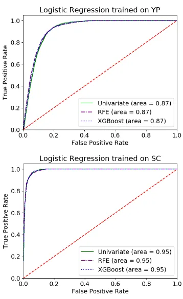
Figure 6.8 ROC curve for Logistic Regression classification trained on

sam-ple unbalanced non-normalized 3-AAU datasets and tested on

full datasets using XGBoost feature importance analysis . . . 88

Figure 6.9 ROC curve for Logistic Regression classification trained on

sam-ple unbalanced non-normalized 3-AAU datasets and tested on

(17)

Figure 6.10 ROC curve for Logistic Regression classification trained on sam-ple unbalanced non-normalized 3-AAU datasets and tested on

full datasets using Univariate analysis . . . 90

Figure 6.11 ROC curve for Random Forest classification trained on sample unbalanced non-normalized 3-AAU datasets and tested on full

datasets using XGBoost feature importance analysis . . . 93

datasets using RFE analysis . . . 94

datasets using Univariate analysis . . . 95

Figure 6.14 ROC curve for XGBoost classification trained on sample unbal-anced normalized 3-AAU datasets and tested on full

non-normalized datasets using XGBoost feature importance analysis . 98

non-normalized datasets using RFE analysis . . . 99

(18)

Chapter 1 Introduction

Proteomics is the study of proteins at a very large scale. The goal of proteomics is to

identify and quantify proteins in a cell. Proteins unlike genomes are dynamic and are

of varying complexity. This is the significant challenge in proteomics. This challenge

is overcome by one of the primary approaches in proteomics, Tandem Mass

Spec-trometry (MS/MS). MS/MS offers high-throughput quantification of the proteome

in a biological sample. However, due to the high-throughput capability of MS/MS,

the cost of performing this analysis on large datasets is significantly large [15].

As described by Web-Robertson et al. [15], there is a significant amount of effort

that goes in to cataloging peptides identified by MS/MS over multiple platforms and

database search routines as the information becomes available (Craig et al., [13];

Desiere et al., [5]; Jones et al., [8]; Kiebel et al., [12]). These database are built over

time and are very helpful in evaluating proteomes for which data has been amassed.

These databases help in reducing cost and time as the search routine to identify

proteotypic peptides has to only run on a subset of possible peptide candidates.

The challenge of building these databases for new organisms remains. To

over-come the very high cost of building these databases, several algorithmic approaches

have been proposed. These algorithms take advantage of the fact that there are many

known properties associated with the likelihood of proteotypic peptides, such as

po-larity, hydrophilicity, hydrophobicity of the peptide. By using the known properties

of the peptides, the challenge of predicting proteotypic peptides are significantly

(19)

model building. In one of the earliest work, Web Robertson et al (2010) [15] used

simple sequence-derived properties of peptides for AMT studies to predict proteotypic

peptides using support vector machine (SVM) classification. The goal of my work is

to improve the prediction of the proteotypic peptides.

In the method described by Web-Robertson et al. [15], the concept of proteotypic

peptides is defined as the peptide that has been included in the AMT database at any

time that the parent protein is observed [15]. We have incorporated one of the three

dataset used by STEPP (Webb-Robertson, 2010) [15] and adopted that definition

of proteotypic peptides. Web-Robertson et al [15] used 35 features in predicting

proteotypic peptides. Table 1.1 lists 35 features from Web-Robertson et al., 2010

[15].

Table 1.1 Proteotypic peptide features. Features 1-35 are from Web-Robertson et

al., 2010 [15] and Feature 36 is from Ahmed Alqurri [11]

Index Features

1 Length

2 Molecular weight

3 Number of non-polar hydrophobic residues

4 Number of polar hydrophilic residues

5 Number of uncharged polar hydrophilic residues

6 Number of charged polar hydrophilic residues

7 Number of positively charged polar hydrophilic residues

8 Number of negatively charged polar hydrophilic residues

9 Hydrophobicity−Eisenberg scale (Eisenberg et al., 1984)

10 Hydrophilicity−Hopp−Woods scale (Hopp and Woods, 1981)

11 Hydrophobicity−Kyte−Doolittle (Kyte and Doolittle, 1982)

12 Hydropathicity−Roseman scale (Roseman, 1988)

13 Polarity−Grantham scale (Grantham, 1974)

14 Polarity−Zimmerman scale (Zimmerman et al., 1968)

15 Bulkiness (Zimmerman et al., 1968)

16−35 Amino acid singlet counts

36 Ordered Amino Acid Usage (3-AAU or 2-AAU)

(20)

(AAU). He was able to achieve similar results to Web-Robertson with only seven

features for theYersinia Pestisdataset. Ordered Amino Acid Usage is an an abstract

model of bonds between adjacent amino acids [11]. Ordered amino acid tuples capture

the mutual information of these peptide fragments at an abstract level [11]. Alqurri

[11] considered both tuples (2-AAU) and triples (3-AAU). We have also adopted that

definition of Ordered Amino Acid Usage.

As already described by Ahmed Alqurri [11], some of the STEPP (Webb-Robertson,

2010) features compliment the AAU approach. We verified that and come up with

different subsets, combining STEPP features and AAU. These subset of features are

slightly different for each of the feature selection methods used in this research. For all

these different feature set we experimented with different machine learning techniques

to get the optimal results for different datasets. Table 1.1 shows all the proteotypic

(21)

Chapter 2 Data Preparation Methodology

We have incorporated Yersinia Pestis dataset from Web-Robertson et al. [15] in

our research. The Saccharomyces cerevisiae (or Yeast) dataset is incorporated from

Ahmed Alqurri [11]. In order to verify and test our classification models, we prepared

one more dataset. We prepared the dataset forBacillus subtilis str. 168. To prepare

the dataset for Bacillus subtilis str. 168, first we downloaded three files

-1. Proteomee file in fasta format from National Center for Biotechnology

Infor-mation (NCBI)

https://www.ncbi.nlm.nih.gov/genome/665/

2. DeepNovo file in mgf format from MassIVE (University of California, San Diego)

[14] Bacillus subtilis str. 168 from

ftp://massive.ucsd.edu/MSV000081382/peak/DeepNovo/HighResolution/data/

3. Observed peptides from Global Proteome Machine Database (GPMDB) [4]

http://peptides.thegpm.org/ /peptides_by_species/

Proteome (fasta) file for Bacillus subtilis str. 168 had total 4,174 observed

pro-teins. DeepNovo file had total 26,687 observed peptides for Bacillus subtilis str.

168 after removing modifications. GPMDB had total 54,069 observed peptides. We

changed the leucine (L) to isoleucine (I) in the proteome (fasta) file as the DeepNovo

file had only isoleucine. We also changed the leucine (L) to isoleucine (I) in the

(22)

We merged the DeepNovo and GPMDB files. We only kept peptides of length

6 or more. We got 18,959 matching peptides from both the files. There were many

smaller peptides which were part of the larger peptides. We checked how many of

these smaller peptides which are present as substrings in larger peptides and are

present in two or more proteins. We found only 36 substrings (smaller peptides)

which were present in two or more proteins, i.e., in one protein they were part of

larger peptide, in other protein(s) they were independent of any existing peptide.

We included only these 36 smaller peptides (substrings) in our proteotypic file for

Bacillus subtilis str. 168 and removed other substrings (smaller peptides) from our

proteotypic file. In the end we had 14,157 proteotypic peptides.

We isolated the GPMDB peptides from Proteome (fasta) file. We digested the

pieces left in the proteome (fasta) file after isolating GPMDB peptides. We removed

the redundancies and kept the peptides of at least length 6. There were total 42,836

peptides left. We classified these 42,836 peptides as non-proteotypic peptides.

The Table 2.1 shows the list of observed and unobserved peptides from Yersinia

Pestis, Saccharomyces cerevisiae and Bacillus subtilis str. 168 datasets.

Table 2.1 Bacterial species protein dataset information

Organisms Y. Pestis S. cerevisiae B. subtilis

Total peptides in identified proteins 113,472 21,514 56,993

Proteotypic peptides 8,073 2,121 14,157

(23)

Chapter 3 A Fast Peptide Classification Using LIBSVM

A support vector machine (SVM) is a supervised learning algorithm that outputs an

optimal hyperplane that categorizes new observations/entries. A SVM can be used

for both classification and regression. In the SVM paradigm each data point is an n

dimensional vector, where n is the number of features. To achieve good classification,

we select a hyperplane (in n dimensional space) that has the largest distance from the

training data of all classes. By having the highest margin, the out-of-sample error is

reduced.

The LIBSVM [2] library is a simple, easy-to-use, and efficient SVM classification

and regression package. We are using the LIBSVM [2] library. The LIBSVM [2]

library is available for many programming languages. We performed support vector

classification (SVC) using the LIBSVM [2] library for C++ and used LIBSVM’s [2]

decision function available in the scikit-learn [10] library for Python. The study for

peptide identification using Ordered Amino Acids with STEPP was done in MATLAB

using it’s built in SVM library by Ahmed Alqurri [11]. The MATLAB code takes

around 12 hours to run. To reduce the time we wrote the same code in C++ and

reduced the time by 7 times.

The LIBSVM [2] has five SVM types:

1. C-SVC (multi-class classification)

2. nu-SVC (multi-class classification)

(24)

4. Epsilon-SVR (regression)

5. nu-SVR (regression)

We have used C-SVC and nu-SVC for classification of peptides into proteotypic

and non-proteotypic peptides.

The LIBSVM [2] supports five kernel types:

1. Linear

2. Polynomial

3. Radial basis function

4. Sigmoid

5. Precomputed kernel

In general, in machine learning a kernel function is used for pattern analysis.

The support vector machine (SVM) is one of the most popular pattern recognition

algorithm that employs a kernel function. Kernel function transforms n dimensional

feature vector (in an algorithms like SVM) to m dimensional feature space, usually

m is much larger than n. Kernel function operates in high dimensional feature space,

by adding new features that are the functions of existing features. Kernel functions

do not calculate coordinates of the data in that high-dimensional space, instead they

calculate the inner products between the images of all the data in that feature space.

This approach is called the "kernel trick".

We have used linear kernel function to achieve similar results as described by Web

(25)

3.1 Motivation: Performance Issues

In previous work, Ahmad Alqurri [11] used MATLAB [9] to achieve Sensitivity of

90% and Specificity of 81% for the Yersinia Pestis dataset. The MATLAB code

was very good for prototyping our ideas, but it soon became a bottleneck as we

set on improving classification metrics. The MATLAB code for SVC with a linear

kernel took approximately 12 hours to run on Intel quad core 2.67GHz processor with

7.8G RAM. Using MATLAB [9] to iterate over our method was a bit time taking.

Improving performance became critical as we worked on feature selection and testing

different classification algorithms on a number of peptide datasets.

We wrote a C++ code using LIBSVM [2] library to get the same results as the

MATLAB [9] implementation of SVM. We have used the normalized datasets for

our experiments reported in this chapter. The performance gain that we achieve

over the MATLAB [9] implementation is significant. The C++ version of code with

nu-SVC reports its results in under 15 minutes. Even for other SVM classifiers

men-tioned above, LIBSVM’s performance is orders of magnitude better compared to

MATLAB [9] implementation.

3.2 Specificity and Sensitivity Metrics

Specificity and sensitivity are statistical metrics to measure performance of binary

classification algorithms. Sensitivity is the true positive rate (TPR) meaning the

per-centage of positives correctly identified. Specificity is the true negative rate meaning

the percentage of negatives correctly identified. Specificity is also defined as1 - False

Positive Rate.

Comparison of specificity and sensitivity for peptides classification with SVM

us-ing LIBSVM and MATLAB are provided in Figure 3.1. We can observe in the figure

(26)

nu-SVC C-SVC MATLAB 10

20 30 40 50 60 70 80 90 100

91 92 ₉₀

81 ₈₀ 81

P

ercen

tage

(%)

Sensitivity (in %) Specificity (in %)

Figure 3.1 Sensitivity and Specificity comparison of LIBSVM [2] and MATLAB [9]

SVM classifiers on Yersinia Pestis dataset.

specificity and sensitivity on Yersinia Pestis dataset. With MATLAB

implementa-tion, we were able to achieve a sensitivity of 90% and specificity of 81%. With the

LIBSVM’s nu-SVC version, we got sensitivity of 91% and specificity of 81%, which

are very similar to MATLAB implementation. With the LIBSVM’s C-SVC version,

(27)

3.3 Speedup with C++ code

We achieved significant speedup with C++ code. The MATLAB code took

approxi-mately 720 minutes to classify Yersinia Pestis dataset. With the LIBSVM’s C-SVC

classification, the time is reduced to 100 minutes. When we implemented the same

LIBSVM’s nu-SVC classification, the time was further reduced to approximately 15

minutes.

LIBSVM nu-SVC 15

LIBSVM C-SVC 100

Matlab SVM 720

0 100 200 300 400 500 600 700 800

Minutes

Figure 3.2 Time taken in minutes for SVM on Yersinia Pestis dataset using three

methods

3.3.1 nu-SVC is faster than C-SVC

We found out that nu-SVC is much faster than C-SVC. nu-SVC takes parameter nu

values between 0 and 1. C-SVC takes parameter C values from 0 to infinity. As the nu

value for nu-SVC can be very small compared to C value for C-SVC, the processing

time for nu-SVC is significantly less than C-SVC. In our model for Yersinia Pestis

dataset, after doing grid search on parameter nu for nu-SVC and C for C-SVC, we

found best results for nu = 0.31 for nu-SVC and C = 1e5 for C-SVC, the sensitivity

(28)

3.3.2 Relative speedups with both algorithms

As shown in the Figure 3.2, nu-SVC takes approximately 15 minutes to complete for

Yersinia Pestisdataset. Whereas, C-SVC takes 100 minutes to complete forYersinia

Pestis dataset.

3.4 Grid Search to get optimal hyper-parameter selection

Hyper-parameters are passed as the arguments to the constructor of the estimator

classes. In LIBSVM [2] support vector classifier the kernel type, degree, gamma, cost,

nu are some of the examples of hyper-parameters. To get the best cross-validation

score, the hyper-parameters are searched and optimized.

Grid search is a method used to search and optimize the hyper-parameters of

the estimator classes. Here in case of support vector classifier for identifying

pep-tides using ordered amino acids, we have optimized the parameter C for C-SVC and

parameter nu value for nu-SVC.

3.4.1 Tuning nu-SVC

The nu-SVC takes C values in the range of 0 to 1. We started our grid search for C

using five values from 0.1 to 0.9 with equal spacing. We found the best results for

C = 0.3. We narrowed grid search for C between 0.2 and 0.4. This time we took

11 numbers between 0.2 and 0.4 with equal spacing for grid search. We found best

sensitivity and specificity for C = 0.31. The results for Sensitivity and Specificity

with C = 0.31 were similar to the Web-Robertson et al. [15] and Ahmed Alqurri [11].

3.4.2 Tuning C-SVC

C-SVC takes C values in the range of 0 to∞. We started our grid search for C using

three values, i.e, 1, 50 and 1e2. We found the best results for C = 1e2. We again did

(29)

1e3. Now we again did grid search with C equal to 1e3, 1e4 and 1e5. In this iteration

we found best results for C = 1e5. The results for Sensitivity and Specificity with

C = 1e5 were very close to the Web-Robertson et al. [15] and Ahmed Alqurri [11].

We stopped our grid search right there but for sanity check we did run our model

with C = 1e6. With C = 1e6, the Sensitivity and Specificity went down by couple

of percentage points. We observed that as we were increasing the value of C for grid

search, the speed of the model was becoming slower.

3.5 Incorporating additional datasets

We incorporated theSaccharomyces cerevisiae dataset in our experiments and

analy-sis. We trained SVC model onSaccharomyces cerevisiaeusing same hyper parameters

as in the Yersinia Pestis model. We used normalized dataset (done using min-max

scalar) for Saccharomyces cerevisiae, similar to Yersinia Pestis dataset. We did

10-fold cross validation. The results were even better than Yersinia Pestis dataset.

We achieved the sensitivity of 97% and specificity of 92% from the Saccharomyces

cerevisiae dataset.

Further we tested our existing SVM classifier trained on Yersinia Pestis dataset

onSaccharomyces cerevisiae dataset but we were getting sensitivity score of

approx-imately 0%. Similarly when we tested the SVM classifier trained on Saccharomyces

cerevisiae with Yersinia Pestis dataset, the specificity was down to approximately

0%. We assumed that the features which we are using for training SVM classifier

here are only giving us the good results for the test sample data taken from the same

datasets.

To get the best results, we did the feature selection from scratch. We used four

feature selection methods:

(30)

Table 3.1 SVC trained on sample balanced 3-AAU datasets and tested on 20% unbalanced datasets Feature Selection Number of Features Classifier Training data Testing

data Sensitivity Specificity

Alqurri [11] 7 SVC Sample YP 20% YP 96% 78%

XGBoost 6 SVC Sample YP 20% YP 94% 79%

RFE 6 SVC Sample YP 20% YP 94% 79%

Univariate 6 SVC Sample YP 20% YP 95% 79%

Alqurri [11] 7 SVC Sample SC 20% SC 97% 92%

XGBoost 6 SVC Sample SC 20% SC 98% 93%

RFE 6 SVC Sample SC 20% SC 97% 93%

Univariate 6 SVC Sample SC 20% SC 97% 92%

2. Recursive Feature Elimination

3. XGBoost feature importance

4. Principal Component Analysis

These feature selection methods are described in detail in Chapter 4.

We have used Scikit-Learn [10] library for python to do further experiments and

analysis. We started off with the Yersinia Pestis datasets. We divided the Yersinia

Pestisdata in to train and test data by 80:20 ratio. We then took balanced data from

80% dataset. We did the feature selection by three different ways: Univariate

Anal-ysis, Recursive Feature Elimination and XGBoost feature importance. For feature

selection we used whole data for Yersinia Pestis.

We first trained the SVM classification model using balanced training data. We

started off with linear kernel. We again did the grid-search on C using scikit-learn

GridSearchCV class with 5 fold cross-validation. We got best results for C = 1e3.

We tested our model on unbalanced 20% of the Yersinia Pestis dataset as well as on

full Yersinia Pestis dataset. We repeated similar steps for Saccharomyces cerevisiae

(31)

3-Table 3.2 SVC trained on sample balanced 3-AAU datasets and tested on full unbalanced datasets Feature Selection Number of Features Classifier Training data Testing

Alqurri [11] 7 SVC Sample YP Full YP 95% 78%

XGBoost 6 SVC Sample YP Full YP 94% 79%

RFE 6 SVC Sample YP Full YP 94% 79%

Univariate 6 SVC Sample YP Full YP 95% 79%

Alqurri [11] 7 SVC Sample SC Full SC 97% 92%

XGBoost 6 SVC Sample SC Full SC 97% 93%

RFE 6 SVC Sample SC Full SC 97% 93%

Univariate 6 SVC Sample SC Full SC 97% 92%

AAU datasets and tested on 20% sample unbalanced datasets. The Figure 3.3 shows

ROC curve with AUC scores for the SVC model trained on sample balanced 3-AAU

datasets and tested on 20% sample unbalanced datasets.

In the next step, we trained the model on sample balancedYersinia Pestisdataset

and tested on fullYersinia Pestiss dataset. We have used 5-fold cross-validation. We

repeated the same steps for Saccharomyces cerevisiae. The Table 3.2 shows SVC

on 3-AAU datasets which is trained on sample balanced datasets but tested on full

datasets using 5-fold cross-validation. The Figure 3.4 shows ROC curve with AUC

scores for the SVC model trained on sample balanced 3-AAU datasets and tested on

full datasets.

After getting good results from models trained on sample balanced dataset, we

trained the model on unbalanced sample ofYersinia Pestis and Saccharomyces

cere-visiaedatasets. For this we trained and tested our models on datasets with 80:20 ratio.

We used the same hyper parameters as was used earlier for training sample balanced

data. We also tested models with full datasets using 5-fold cross-validation. The

Table 3.3 and Table 3.4 shows the SVC models trained on 80% unbalanced datasets

(32)

(33)

(34)

Table 3.3 SVC trained on sample unbalanced 3-AAU datasets and tested on 20% unbalanced datasets Feature Selection Number of Features Classifier Training data Testing

Alqurri [11] 7 SVC Sample YP 20% YP 96% 78%

XGBoost 6 SVC Sample YP 20% YP 94% 79%

RFE 6 SVC Sample YP 20% YP 94% 79%

Univariate 6 SVC Sample YP 20% YP 95% 79%

Alqurri [11] 7 SVC Sample SC 20% SC 97% 92%

XGBoost 6 SVC Sample SC 20% SC 98% 93%

RFE 6 SVC Sample SC 20% SC 97% 93%

Univariate 6 SVC Sample SC 20% SC 97% 92%

Table 3.4 SVC trained on sample unbalanced 3-AAU datasets and tested on full

unbalanced datasets Feature Selection Number of Features Classifier Training data Testing

Alqurri [11] 7 SVC Sample YP Full YP 95% 78%

Alqurri [11] 7 SVC Sample SC Full SC 97% 92%

ure 3.5 and Figure 3.6 shows ROC curve with AUC scores for the SVC trained on

80% sample unbalanced 3-AAU datasets and tested on 20% sample datasets and full

datasets.

We then incorporated both the datasets from Yersinia Pestis and Saccharomyces

cerevisiae to test our models. We found that our model trained on only 6 features

of Yersinia Pestis is not classifying Saccharomyces cerevisiae dataset that well for

3-AAU datasets. The AUC score when we were training and testing using datasets

(35)

(36)

(37)

Table 3.5 SVC on 3-AAU datasets trained and tested on datasets from different species with three different feature selection methods and using RBF kernel

Feature Selection Number of features Classifier Training data Testing

XGBoost 13 SVC Sample YP Full SC 90% 82%

XGBoost 13 SVC Sample SC Full YP 86% 74%

RFE 13 SVC Sample YP Full SC 90% 82%

RFE 13 SVC Sample SC Full YP 86% 73%

Univariate 13 SVC Sample YP Full SC 86% 83%

Univariate 13 SVC Sample SC Full YP 87% 71%

performed feature selection using XGBoost feature importance, Univariate and RFE

on combined features for Yersinia Pestis and Saccharomyces cerevisiae. We did this

to make sure that both the models are trained on the same feature sets.

We again performed grid search with 5-fold cross-validation on kernel, C and

gamma. For both the Yersinia Pestis and Saccharomyces cerevisiae dataset, we get

best results for Radial Basis Function (RBF) kernel with C = 0.1 and gamma =

auto. We have also used the 5-fold cross-validation. We have tested the model on

the dataset from different species. The Table 3.5 shows Support Vector Classification

using different feature selection methods, tested on datasets from different species.

The Figures 3.7, 3.8 and 3.9 show the AUC scores for the SVC done on the

normalized datasets using XGBoost feature importance analysis, Recursive feature

elimination and Univariate Analysis. We have used 13 features from all three feature

selection methods to achieve these results.

We also performed principal component (PCA) analysis for feature reduction on

(38)

(39)

(40)

(41)

(42)

Table 3.6 SVC on 3-AAU datasets tested on datasets from different species with 8 principal components and RBF kernel

Feature Selection

Principal

Components Classifier

Training data

Testing

data Sensitivity Specificity PCA 8 SVC Sample YP Full SC 88% 84% PCA 8 SVC Sample YP Full YP 89% 75% PCA 8 SVC Sample SC Full SC 95% 89% PCA 8 SVC Sample SC Full YP 86% 66%

used all 3-AAU dataset features to get 8 principal components that gave us good

results. The 8 principal components from Yersinia Pestis model covered 84% of the

variance. For the model trained on the Saccharomyces cerevisiae dataset, 80% of the

variance was covered. For SVM classification, we have used RBF kernel with C = 1

and gamma = auto. We have used the 5-fold cross-validation. We have tested the

model with both the datasets.

The Table 3.6 shows Support Vector Classification (SVC) using 8 principal

com-ponents on 3-AAU datasets and tested on datasets from different species. The Figure

3.10 shows ROC curve with AUC score for Support Vector Classification shown in

(43)

Chapter 4 Feature Selection

Feature selection demonstrates that only small set of features are required for correct

prediction of proteotypic peptides. Feature selection is also very important to decrease

cost of running models on very big data. Web-Robertson et al. [15] performed support

vector classification using all the features but they did provide Fisher Criterion Score

(FCS) [1] for each feature. They also mentioned that less number number of features

would also provide good prediction of proteotypic peptides. Web-Robertson et al. [15]

didn’t perform feature selection through algorithms like recursive feature elimination

(RFE) because of high cost of computation required to run them on big data.

Ahmed Alqurri [11] performed support vector classification only on 7 features.

Alqurri used linear discriminate analysis (LDA) and examined LDA loadings to see

the contributions of each feature. After examining LDA loadings, they came up with

7 features. We decided to do features selection exhaustively.

We performed four types of feature selections and did classification using all these

sets of features. In this chapter we have used normalized datasets (done through

min-max scalar) for feature selection. The four feature selection method we used are

as below

-1. Univariate Analysis

2. Recursive Feature Elimination

3. XGBoost feature importance

(44)

4.1 Univariate Feature Selection

Figure 4.1 Chi2 score for feature selection on 3-AAU Yersinia Pestis dataset

Univariate feature selection is based on univariate statistical analysis. Univariate

analysis deals with only one variable at a time. It doesn’t deal with the relationship

between features or variables. Univariate analysis is used to summarize data. The

scikit-learn [10] Python library provides SelectKBest class that can be used with

different statistical tests to select a specific number of features. SelectKBest returns

a subset of the highest scoring features.

We have used the basic chi-squared test as a scoring function with the

scikit-learns [10] SelectKBest class to select features. The chi-squared statistic or χ2 test

removes features which are mostly independent of the class and therefore irrelevant

(45)

Figure 4.2 Chi2 score for feature selection on 3-AAU Saccharomyces cerevisiae

dataset

[6] in 1900. The chi-squared test is a statistical hypothesis test where the statistical

distribution of the test statistic is a chi-squared distribution where the null hypothesis

is true. The null hypothesis in case of a chi-squared test is defined as the hypothesis

that states there is no significant difference between expected and observed data.

In our case, we are performing a chi-squared test for independence to test if a

particular feature in our data is independent of the class. If that feature is independent

of the class then we remove that feature from the classification. The chi-squared

statistic is a number that signifies whether the observed value would be significantly

different from the expected value if there was no relationship. If the chi-squared

statistic is low then it signifies that there is a relationship between a feature and the

(46)

Figure 4.3 Chi2 score for feature selection on 3-AAU Yersinia Pestis and

Saccharomyces cerevisiae dataset

a feature and class.

The chisquared statistic for the chisquared test is calculated by the formula

-χ2_f =X(Oi−Ei)

2

Ei

(4.1)

where f is the degree of freedom, O is the observed value and E is the expected value.

We performed Univariate analysis for Yersinia Pestis, Saccharomyces cerevisiae

and dataset containing the features from both Yersinia Pestis and Saccharomyces

cerevisiae. The Figures 4.1, 4.2 and 4.3 show the feature selection scores from

uni-variate analysis we have done on three datasets. From the uniuni-variate analysis we can

observe that number of proline (P) residues and ordered amino acid usage (3-AAU)

(47)

4.2 Recursive Feature Elimination

Figure 4.4 RFE feature ranks for 3-AAU Yersinia Pestis dataset

Recursive Feature Elimination (RFE) is a multivariate feature selection method.

RFE removes features recursively and build the model using the remaining features

that are left behind. RFE uses an external estimator to build a model that assigns

weights to features. It ranks the features either through coef_ attribute or through

feature_importance_ score. The features with least scores are removed from current

set of features. This process is repeated recursively with reduced features until the

re-quired set of features are selected. As such, this is a greedy algorithm to select the best

performing features. Scikit-learn’s [10] provides RFE class under feature_selection

library. We implemented RFE with logistic regression to rank features by weights.

(48)

Figure 4.5 RFE feature ranks for 3-AAU Saccharomyces cerevisiae dataset

cerevisiae and combination of calculated features from bothYersinia Pestis and

Sac-charomyces cerevisiae. The Figures 4.4, 4.5 and 4.6 show the feature rankings for

Re-cursive Feature Elimination (RFE) we have done on three datasets. For bothYersinia

Pestis andSaccharomyces cerevisiae, feature number 35 i.e, Ordered Amino Acid

(3-AAU) ranked at the top followed by Hydrophobicity-Eisenberg scale (Eisenberg et

al., 1984), Hydrophilicity-Hopp-Woods scale (Hopp and Woods, 1981) and

Polarity-Grantham scale (Polarity-Grantham, 1974). For the combined calculated features dataset

for Yersinia Pestis and Saccharomyces cerevisiae, ordered amino acid (3-AAU) still

tops the rank, but second, third and fourth position goes to Number of positively

charged polar hydrophilic residues, Hydropathicity-Roseman scale (Roseman, 1988)

(49)

Figure 4.6 RFE feature ranks for on 3-AAU Yersinia Pestis and Saccharomyces cerevisiae dataset

4.3 XGBoost feature importance

XGBoost stands for Extreme Gradient Boosted trees. XGBoost is a supervised

learn-ing technique used for classification and regression. More details are given in section

5.4.

XGBoost library [3] in python provides a very useful function feature_importance_

for trained model. These importance scores are calculated when the model is getting

trained. These importance scores are F scores for each feature. These importance

scores can be calculated by three types [3]: ’weight’, ’gain’ and ’cover’. ’weight’ is the

number of times a feature is used to split the data across all trees [3]. ’gain’ is the

(50)

Figure 4.7 XGBoost feature importance for 3-AAU Yersinia Pestis dataset

Figure 4.8 XGBoost feature importance for 3-AAU Saccharomyces cerevisiae

(51)

Figure 4.9 XGBoost feature importance for on 3-AAU Yersinia Pestis and

Saccharomyces cerevisiae dataset

of the feature when it is used in trees [3]. We have used ’weight’ as the importance

type to calculate the feature importance score.

We generated XGBoost feature importance scores for Yersinia Pestis,

Saccha-romyces cerevisiae and combined features from both Yersinia Pestis and

Saccha-romyces cerevisiae datasets. The Figures 4.7, 4.8 and 4.9 show the feature

impor-tance scores from XGBoost models we ran three datasets. For all the three datasets,

feature number 35 and 1 i.e, Ordered Amino Acid (3-AAU) and molecular weights of

the peptides have the highest scores.

4.4 Principal Component Analysis

Principal Component Analysis (PCA) is an unsupervised learning method used for

multivariate analysis. Principal Component Analysis (PCA) is a statistical method

that reduces the multivariate dataset in to a set of multiple orthogonal components

(52)

of data while retaining most of the original information. PCA is mathematical tool

that reduces high number of correlated features in to less uncorrelated orthogonal

principal components. In other words, PCA is a linear dimension reduction tool that

is very useful for data with high correlated variables.

Figure 4.10 PCA feature reduction on 3-AAU Yersinia Pestis and Saccharomyces

(53)

PCA was first invented by Karl Pearson in 1901 [6] and later developed by Harold

Hotelling in the 1936 [7]. PCA is one of the simplest eigenvector based multivariate

analysis. PCA is mostly used in explanatory data analysis. We have implemented

PCA using pythons scikit-learn [10] library. Scikit-learn [10] uses the LAPACK

imple-mentation of the full Singular Value Decomposition (SVD) or a randomized truncated

SVD by the method of Halko et al. 2009, depending on the shape of the input data

and the number of components to extract. It also has option of the scipy.sparse.linalg

ARPACK implementation of the truncated SVD [10].

We did Principal Component Analysis (PCA) for Yersinia Pestis and

Saccha-romyces cerevisiae datasets. The Figure 4.10 show the explained variance from PCA

analysis we have done on two datasets. In the figure 4.10, n_components is the

num-ber principal components and explained_variance_ratio_ is the variance explained

by each principal component. In figure 4.10, the graphs flattens out from principal

components 7. These 7 components covers around 82% variance for Yersinia Pestis

(54)

Chapter 5 Machine Learning techniques for peptide

classification

We did experiments using four different machine learning algorithms to verify if

Sup-port Vector Machine (SVM) is giving us the best peptide classification. We have

incorporated Saccharomyces cerevisiae dataset to train and test our models in

addi-tion to Yersinia Pestis dataset. The following are the machine learning algorithms

which we have performed for this research:

1. Logistic Regression

2. Random Forest

3. K-Nearest Neighbor

4. XGBoost

We have also performed three different feature selection techniques to come up

with optimal features as described in Chapter 4. The three feature selection

meth-ods we performed are Univariate Analysis, Recursive Feature Elimination (RFE) and

XGBoost (via it’s feature importance method). We have also performed feature

reduction algorithm, Principal Component Analysis (PCA). We are reporting the

results from each of the classification method using different feature selection

meth-ods. We started to run our experiments on normalized datasets. We performed the

(55)

We have performed our tests on Yersinia Pestis and Saccharomyces cerevisiae

(Yeast) normalized datasets. We started off by dividing each of the datasets in to

train and test data by 4:1 ratio. We have also tested each of our trained models with

both the data sets. We have used grid search with cross-validation to come up with

optimal parameters for each of the classifiers. For all these analysis we have used

scikit-learn [10] package for Python.

We will go in to each of the classification methods in more detail

below:-5.1 Logistic Regression

Logistic Regression is a supervised learning technique. Logistic regression is a

classi-fier that classifies an observation in one of the two or more classes. Logistic regression

can be binomial, multinomial or ordinal. In our case, we are using binomial logistic

regression. The logistic function is at the core of logistic regression. The logistic

function is a ’S’ shaped sigmoid curve. The equation of logistic function is as, with

x as a real value number between−∞ to +∞.

f(x) = e

x

(1 +ex₎ (5.1)

A logistic regression is a model which provides log-odds of the probability of an

event in a linear combination of independent or predictor variables. Binary logistic

regression is an expression of probability of an event Y = 1, 0 occurring against a set

of X = (X1, X2, ..., Xk) explanatory variables which can be discrete, continuous, or

a combination.

logit(P r(Yi = 1|Xi =xi)) =logit(πi) = β0+β1xi1+...+βkxik (5.2)

We started off with the Yersinia Pestis datasets. We divided the Yersinia Pestis

dataset in to train and test data by 80:20 ratio. We then took balanced data from 80%

(56)

Table 5.1 Logistic Regression trained on sample balanced 3-AAU datasets and tested on 20% unbalanced datasets

Feature Selection Number of Features Classifier Training data Testing

XGBoost 6 Logistic Regression Sample YP 20% YP 94% 80%

RFE 6 Logistic Regression Sample YP 20% YP 94% 80%

Univariate 6 Logistic Regression Sample YP 20% YP 94% 80%

XGBoost 6 Logistic Regression Sample SC 20% SC 96% 94%

RFE 6 Logistic Regression Sample SC 20% SC 97% 94%

Univariate 6 Logistic Regression Sample SC 20% SC 97% 94%

Recursive Feature Elimination (RFE) and XGBoost feature importance. For feature

selection we used the whole dataset for Yersinia Pestis. We trained the Logistic

Regression using balanced training data. We tested our model on unbalanced 20% of

theYersinia Pestisas well as on fullYersinia Pestisdataset. We did the grid search on

the trained model to optimize the results. We did grid search with cross-validation

on the three parameters: penalty, C and solver. We have also used 10-fold

cross-validation while training our models. We repeated similar steps from feature selection

to model training on Saccharomyces cerevisiae dataset. The Table 5.1 shows Logistic

Regression on sample balanced 3-AAU datasets and tested on 20% of the unbalanced

datasets. The Figure 5.1 shows ROC-AUC curve for the Logistic Regression on sample

balanced 3-AAU datasets and tested on 20% of the unbalanced datasets.

In the next step, we trained the Logistic Regression model on sample balanced

Yersinia Pestis dataset but tested it on full Yersinia Pestiss dataset with 10-fold

cross-validation. We repeated the same steps for Saccharomyces cerevisiae. For the

model trained on Yersinia Pestis, feature selection is done using Yersinia Pestis

dataset. For the model trained onSaccharomyces cerevisiae, feature selection is done

using Saccharomyces cerevisiae dataset. The Table 5.2 shows Logistic Regression

on 3-AAU datasets which is trained on sample balanced 3-AAU datasets but tested

(57)

(58)

Table 5.2 Logistic Regression trained on sample balanced 3-AAU datasets and tested on full unbalanced datasets

XGBoost 6 Logistic Regression Sample YP Full YP 93% 79%

RFE 6 Logistic Regression Sample YP Full YP 94% 79%

Univariate 6 Logistic Regression Sample YP Full YP 94% 80%

XGBoost 6 Logistic Regression Sample SC Full SC 97% 93%

RFE 6 Logistic Regression Sample SC Full SC 97% 93%

Univariate 6 Logistic Regression Sample SC Full SC 97% 92%

tic Regression on sample balanced 3-AAU datasets and tested on full unbalanced

datasets.

After getting good results from logistic regression models trained on sample

bal-anced data, we trained the model on unbalbal-anced sample of Yersinia Pestis and

Sac-charomyces cerevisiae datasets. For this we trained and tested our models on 80:20

ratio. We used the same hyper parameters as used earlier for training sample

bal-anced data. For unbalbal-anced datasets, we have used class weights. Like previously

we also tested our models on full datasets using 10-fold cross-validation. The Tables

5.3 and 5.4 shows the Logistic Regression results trained on 80% unbalanced datasets

and tested on 20% data and full datasets respectively. The Figures 5.3 and 5.4 shows

the ROC-AUC curve for the Logistic Regression results trained on 80% unbalanced

datasets and tested on 20% data and full datasets respectively.

We then incorporated both the datasets from Yersinia Pestis and Saccharomyces

cerevisiae to test our logistic regression models. We found that our model trained

on only 6 features of Yersinia Pestis dataset is not able to classify Saccharomyces

cerevisiae dataset that well for 3-AAU datasets. Similarly, the model trained on

Sac-charomyces cerevisiae was not able to classify the Yersinia Pestis dataset that well.

The AUC score when we were training and testing using datasets from two different

(59)

se-Figure 5.2 ROC curve for Logistic Regression trained on sample balanced 3-AAU datasets and tested on full unbalanced datasets using three different feature

(60)

(61)

(62)

Table 5.3 Logistic Regression trained on sample unbalanced 3-AAU datasets and tested on 20% unbalanced datasets

XGBoost 6 Logistic Regression 80% YP 20% YP 94% 80%

RFE 6 Logistic Regression 80% YP 20% YP 94% 80%

Univariate 6 Logistic Regression 80% YP 20% YP 94% 80%

XGBoost 6 Logistic Regression 80% SC 20% SC 96% 94%

RFE 6 Logistic Regression 80% SC 20% SC 97% 94%

Univariate 6 Logistic Regression 80% SC 20% SC 97% 94%

Table 5.4 Logistic Regression trained on sample unbalanced 3-AAU datasets and

tested on full unbalanced datasets

XGBoost 6 Logistic Regression 80% YP Full YP 93% 79%

RFE 6 Logistic Regression 80% YP Full YP 94% 79%

Univariate 6 Logistic Regression 80% YP Full YP 94% 80%

XGBoost 6 Logistic Regression 80% SC Full SC 97% 93%

RFE 6 Logistic Regression 80% SC Full SC 97% 93%

Univariate 6 Logistic Regression 80% SC Full SC 97% 92%

lection using XGBoost feature importance, Univariate and RFE on combined features

for both the Yersinia Pestis and Saccharomyces cerevisiae datasets. We did this to

make sure that both the model are trained on the same feature sets. The results for

3-AAU datasets were not good, the AUC scores were pretty low.

We created the 2-AAU datasets forYersinia Pestis andSaccharomyces cerevisiae

for further testing. We again performed feature selection using XGBoost feature

im-portance, Univariate and RFE on combined features forYersinia Pestis and

Saccha-romyces cerevisiae 2-AAU normalized datasets. We again performed grid search with

5-fold cross-validation on C and penalty. We have used class weights. We got decent

(63)

2-Table 5.5 Logistic Regression trained on sample unbalanced 2-AAU datasets tested on full unbalanced datasets from different species. The feature selection is done

using features from both the Yersinia Pestis and Saccharomyces cerevisiae datasets.

RFE 13 Logistic Regression Sample YP Full SC 92% 50%

RFE 13 Logistic Regression Sample YP Full YP 72% 74%

RFE 13 Logistic Regression Sample SC Full SC 85% 77%

RFE 13 Logistic Regression Sample SC Full YP 69% 75%

Table 5.6 Logistic Regression trained on sample unbalanced 3-AAU datasets and

tested on full unbalanced datasets from different species

Feature Selection Principal Components Classifier Training data Testing

PCA 8 Logistic Regression Sample YP Full SC 81% 78%

PCA 8 Logistic Regression Sample YP Full YP 85% 75%

PCA 8 Logistic Regression Sample SC Full SC 91% 80%

PCA 8 Logistic Regression Sample SC Full YP 83% 68%