on Real Materials
Nils-Oliver Linden
on Real Materials
Nils-Oliver Linden
Dissertation
an der Fakultät der Physik
der Ludwig–Maximilians–Universität
München
vorgelegt von
Nils-Oliver Linden
aus Wilhelmshaven
Numerische Untersuchungen stark korrelierter fermionischer Systeme sind schwierig und beinhalten noch heute essentielle Probleme. Die Hauptgründe dafür sind das exponen-tielle Wachstum des Hilbertraumes der Quantenzustände mit der Systemgröße und das fermionische Vorzeichenproblem bei Monte-Carlo-Rechnungen. Eine der am häufigsten verwendeten Methoden zur Untersuchung zweidimensionaler Gittersysteme sind Cluster-Erweiterungen der dynamische Molekularfeld Theory (DMFT), wie zum Beispiel die dy-namische Cluster Approximation (DCA). Diese Methoden bilden mehrdimensionale Git-tersysteme auf eindimensionale Störstellen-Probleme ab. 2015 wurde gezeigt, dass DMFT auf der imaginären Frequenzachse kombiniert mit der Dichtematrix-Renormierungsgruppe (DMFT+DMRG) Mehrband- und Multisite-Systeme schneller lösen kann, als wenn an-dere Störstellen-Löser verwendet werden.
In dieser Arbeit entwickeln wir diesen Ansatz weiter und wenden ihn auf Modelle realer Materialen an. Am Anfang dieser Arbeit besprechen wir relevante Methoden für DMRG+ DMFT, wie zum Beispiel Matrix-Produkt-Zustände, die Dichtematrix-Renormierungs-gruppe und mehrere Zeitentwicklungs-Methoden. In diesem Zusammenhang werden wir auch mehrere Verbesserungen besprechen, die von methodischen Anpassungen von Zeit-entwicklungen bis hin zur Neuordnung des Tensornetzwerkes basierend auf Verschrän-kungs-Eigenschaften reichen. Danach werden wir uns detailliert mit den methodologischen und programmiertechnischen Aspekten von DMFT beschäftigen. Dieses Kapitel dient als Grundlage für andere Forscher, die eigene DMRG+DMFT-Codes programmieren wollen. Abschließend werden wir drei verschiedene Modelle besprechen, um das Ausmaß der Sys-teme zu zeigen, die mit diesem Ansatz gelöst werden können. Wir werden uns im Kon-text des Hubbard-Modells detailliert mit Multisite-DCA beschäftigen und zeigen, dass DMRG+DMFT Ergebnisse für Systeme mit mittleren Wechselwirkungsstärken bei niedri-gen Temperaturen erzeuniedri-gen kann. Das ist mit anderen Störstellen-Lösern bisher nicht möglich. Im zweiten Fall beschäftigen wir uns mit Strontiumvanadat Sr2VO4 und werden
die ersten Zweisite-DCA-Ergebnisse für ein realistisches Dreiband-Modell präsentieren. Im Gegensatz zu bisherigen Erwartungen führt die teilweise Wiedereinführung der Im-pulsabhängigkeit der Selbstenergie nicht zu einer besseren Übereinstimmung von Theorie und Experiment. Das dritte Modell beschreibt Strontiumruthenat Sr2RuO4. In diesem
Numerical studies on strongly correlated fermionic systems are very complicated and still provide essential problems. The main reason is the exponential growth of the un-derlying Hilbert state space with the system size and the fermionic sign problem for Monte Carlo studies. Among the most widely employed numerical techniques for study-ing two-dimensional quantum many-body systems are cluster extensions of the dynamical mean-field theory (DMFT), e.g. dynamical cluster approximation (DCA). They map an infinitely large multi-dimensional lattice problem to a one-dimensional impurity problem. In 2015 it was shown that the density matrix renormalisation group (DMRG) used as an impurity solver for DMFT (DMFT+DMRG) on the imaginary-frequency axis allows to solve multi-site and multi-band problems extremely fast compared to other solvers. Within this thesis, we further develop this DMRG+DMFT approach to apply the method on real material settings. The step from artificial, completely degenerate multi-band mod-els with simple dispersion relations on a Bethe lattice, studied in 2015, to systems with realistic band structures and lifted degeneracies involves more challenges than originally suspected.
In this thesis, we will first recapitulate relevant methods for our approach like matrix prod-uct states, the density matrix renormalisation group and several time evolution methods. In this context we will present several improvements ranging from optimised time evo-lutions to entanglement based optimisations of tensor networks. Second, we will present a very detailed description of the dynamical mean field theory. We will focus on both methodological aspects and implementation details. This chapter is intended to allow other researcher to implement their own DMFT code using DMRG as an impurity solver. Third, we will discuss three different models to show the extent of problems DMRG+ DMFT is able to solve. We will focus on multi-site DCA calculations in the case of the two-dimensional Hubbard model and show that DMRG allows to tackle systems with intermediate interaction strengths at low temperatures, which are unsolvable with other solvers. In the second case, the real material Sr2VO4, we will show the first two-site DCA
results for a realistic three-band model. In contrast to assumptions, partly reintroducing the momentum dependence of the self-energy does not improve agreement between exper-imental observations and theoretical results. Finally, we will move on to another realistic three-band model, which describes Sr2RuO4, to show how to deal with the influence of
1 Introduction 1
2 Tensor Networks 7
2.1 Matrix Product States . . . 8
2.2 Matrix Product Operators . . . 16
3 Density Matrix Renormalisation Group 19 3.1 Single-Site-DMRG . . . 20
3.2 Strictly Single-Site DMRG . . . 23
3.3 Optimal Order of Tensors . . . 25
3.4 Other Network Topologies . . . 31
4 Time Evolution Methods 35 4.1 Time Evolution with Block Decimation . . . 36
4.2 Krylov Approximation . . . 39
4.2.1 Variational Orthogonalisation . . . 41
4.2.2 Tensor-Optimised Implementation . . . 43
4.2.3 Reusing the Krylov-Subspace . . . 45
4.2.4 Conclusion . . . 47
4.3 Time-Dependent Variational Principle . . . 47
4.4 Long Time Behaviour . . . 50
4.4.1 Linear Prediction . . . 51
4.4.2 Projection of Low Energy States . . . 53
5 Dynamical Mean-Field Theory 57 5.1 Baym-Kadanoff Equations . . . 59
5.2 Impurity Solvers . . . 61
5.3 Step By Step: A Full DMFT Iteration . . . 66
5.3.1 Hybridisation . . . 66
5.3.2 Ground State Calculation . . . 72
5.3.3 Matsubara Green’s Functions . . . 77
5.3.4 Self-Consistency Equation . . . 86
5.3.6 Convergence and Real Frequency Green’s Function . . . 91
5.4 Dynamical Cluster Approximation . . . 97
6 The Two-Dimensional Hubbard Model 103 6.1 The Hubbard Hamiltonian . . . 105
6.2 Bath Size . . . 111
6.3 Comparison with CTQMC Results . . . 115
6.4 DCA with Eight Sites . . . 119
6.5 Intermediate Interaction Strengths . . . 121
6.6 Summary . . . 125
7 A Real Material Study: Sr2VO4 127 7.1 The Hubbard-Kanamori Hamiltonian . . . 128
7.2 Single-Site DMFT and Two-Site DCA . . . 136
7.3 Summary . . . 143
8 Spin-Orbit coupling: Sr2RuO4 145 8.1 The Hamiltonian . . . 146
8.2 Basis Transformation . . . 150
8.3 Fitting of Matrix-Valued Hybridisations . . . 154
8.4 Comparison between DMFT and CTQMC without SOC . . . 159
8.5 The Influence of Spin-Orbit Coupling . . . 164
8.6 Conclusion . . . 166
9 Conclusion 169
Acknowledgements 173
List of Figures 175
List of Tables 177
Introduction
The aim of Quantum mechanics is to understand and predict the behaviour of electrons, atoms, photons and molecules at atomic scales. In turn, this determines the macroscopic properties of materials such as, for example, electrical and thermal conductivity, and re-sistance as well as their magnetic behaviour. Condensed matter theory focuses on trying to understand the origin of these properties and determining how they are influenced by the spatial distribution of atoms and orbitals in unit cells, temperature, pressure, doping and other parameters. With this knowledge at hand one can deliberately identify or de-sign compounds that exhibits certain characteristics under clearly defined conditions. Many of these properties are interesting because they promise to lead to new technical revolutions similar to how the understanding of semi-conductors in the last century led to the development of computers, smartphones and microcontrollers. A comparable un-derstanding of strongly correlated materials could for instance allow to design compounds that are tuned close to phase transitions and react extremely fast to parameter changes like applied currents or pressure. This would decrease the amount of energy needed to control these devices and lower their response times significantly[1,2,3] compared to semi
conductors. Another interesting phenomenon is high-temperature superconductivity. Un-derstanding the mechanisms behind this behaviour could allow to design materials that exhibit this property at room temperature, which definitely would change our society dramatically[4,5,6].
However, the wide variety of interaction types and strengths between electrons and be-tween electrons and atoms give rise to an enormous range of different physical phenom-ena[7,8,9,10,11,12]. Studies of strongly correlated materials are very complicated and
relevant aspects since the difficulty and runtime of computations is affected strongly by the complexity of the model. This leads us to the second step: The model has to be solved. While multiple methods exist that produce results for one-dimensional problems very efficiently such as density matrix renormalisation group[13], exact diagonalisation[14]
or continuous time quantum Monte Carlo[15], in general, two-dimensional problems still
provide significant problems and three-dimensional models are not solvable at all.
Recent years have seen great interest in two-dimensional quantum many-body systems in both theoretical and experimental physics. On the theoretical side, new non-perturbative approaches are developed[16,17,18] inspired by ideas of different fields. With the help of
quantum information theory more efficient tensor networks are invented[19], quantum
chemistry provides useful insights on highly correlated models and optimal representa-tions of quantum problems[20,21], while machine learning techniques are used to study
quantum many-body states[22,23,24] and to optimise existing numerical techniques[25]. On
the experimental side, developments in the field of cold atomic gases and quantum optics allow for the setup and manipulation of quantum lattice systems under controlled and repeatable conditions[26]. This opens completely new possibilities for comparisons and
mutual influence between experiment and theory for future research.
These developments are not only interesting from a theoretical point of view but also lead to an increasing amount of research on more and more complex and realistic solid state models. Accordingly, the demand for numerical resources is strongly increasing and many numerical methods that have been very successful so far seem to have reached their lim-its. Correspondingly, many improvements to these kinds of methods are being developed and are still the main focus of many researchers. However, the most reliable methods to study quantum-mechanical systems so far, exact diagonalisation[27] and Monte Carlo
sampling[28], still encounter large difficulties. The former is limited by the exponential
growth of the Hilbert state space and fails to tackle relevant systems sizes. The latter is often limited by the so-called sign problem that is encountered in many fermionic systems. If present, it prevents Monte Carlo from determining the behaviour of complex models at low enough temperatures. Among the most widely employed numerical techniques for studying quantum many-body systems are the dynamical mean-field theory[29,30,31]
(DMFT) and its cluster extensions, e.g. dynamical cluster approximation[32,33] (DCA).
and more similar to the original lattice problem. Unsurprisingly, that causes computation times to increase exponentially.
DMFT is successful because of two main reasons: First, over the time it was shown that many models and materials are well described by DMFT results, despite the fact that self-energies are momentum-independent. Second, the success and failure of DMFT for arbitrary systems depends strongly on the method chosen to solve the auxiliary impurity problem, also called impurity-solver. There exist a wide variety of impurity solvers that make DMFT so flexible and versatile. The most prominent examples are continuous time quantum Monte Carlo[34] (CTQMC), exact diagonalisation[14] (ED), the numerical
renor-malisation group (NRG)[35] and the density matrix renormalisation group (DMRG)[17,36]
CTQMC is widely and very successfully used as an impurity solver. Unfortunately, com-puting low-temperature results is computationally highly expensive and limits the use of CTQMC in many cases to unsuitable high temperatures. Since CTQMC solves the impurity problem on the imaginary-frequency axis, calculating real-frequency quantities requires analytical continuations. Unfortunately, they are numerically ill-posed and suffer from severe practical difficulties. Furthermore, the application of CTQMC in some cases is highly limited by the fermionic sign problem, which often occurs for systems with mul-tiple relevant orbitals, non-Hubbard interactions or large cluster DCA calculations at low temperatures.
Exact diagonalisation solves the impurity problem on the imaginary-frequency axis with-out making any kind of assumptions. It suffers under no general limitations and is only restricted by the size of the Hilbert space of the impurity problem. This restrains the num-ber of correlated impurity sites and associated bath sites that describe the non-interacting environment. In practice, this limits ED to systems with only a couple of relevant orbitals and small cluster DCA calculations, albeit there have been recent developments with re-stricted Hilbert spaces[37,38] that increase accessible systems sizes slightly.
In contrast to the previous two methods, NRG solves the auxiliary problem on the real-frequency axis and obtains high-quality results for the low-real-frequency limit especially. Due to its way of solving the impurity problem, NRG is limited strongly by the number of correlated sites, which hardly can exceed one or two impurity sites. Only recently NRG was pushed to solve a three-band problem in the context of DMFT[18] but it remains
questionable how far it can be extended.
The density matrix renormalisation group (DMRG) was first used as an impurity solver for DMFT in 2004[36,39]. In contrast to NRG, the high-quality results obtained on the
solve a three-band model on the real-frequency axis with DMRG[40]. However, it is still in
questionable whether DMRG+DMFT is able to solve multi-band models or higher-order DCA calculations of real materials.
Wolf et al. in 2015[17] followed a different road by proposing to solve DMFT on the
imaginary-frequency axis with DMRG. While impurity problems on the real-frequency axis consists of 60 to 100 bath sites per correlated site, on the imaginary axis only three to ten are necessary for an excellent description of the non-interacting environments. Wolf et al. showed that these small systems lead to very fast runtimes compared to other solvers and at the same time to remarkable agreements with CTQMC results. Instead of using analytic continuations to obtain real-frequency results after DMFT is converged, they pro-posed to perform an additional real-frequency calculation based on the converged impurity problem. With this approach they were able to compute the first spectral functions of a completely degenerate three-band Hubbard-Kanamori model at zero temperature with a two-site DCA calculation. The results were not of a high quality but allowed to determine whether a system is an insulator or a metal. Albeit this system was far from being realis-tic, the remarkably short computations times indicated that more complex and realistic models could be solvable with this ansatz. Thus, they proposed to use DMRG+DMFT on the imaginary axis as an effective low-cost solver for DMFT and DCA problems that were not accessible with other impurity solvers.
Within this thesis, we further develop DMRG+DMFT on the imaginary-frequency axis to be able to apply the method on real material settings. The step from a completely degenerate multi-band problem with a simple dispersion relation on a Bethe lattice to a system with a realistic band structure and lifted degeneracies involved more challenges than originally suspected. The entanglement growth is significant, convergence problems occur due to more complex phases being present and symmetries become more important for the performance and convergence of DMFT. Therefore, to obtain results for real ma-terial models, it is necessary to improve methodological aspects such as, for example, a better Krylov method for computing time evolutions or model representations such as the reordering of the lattice sites based on entanglement properties. Additionally, improv-ing implementational details such as optimised parallelisations and determinimprov-ing which symmetry quantum numbers can and should be implemented is also necessary to obtain results for most model calculations.
We will begin this thesis by introducing matrix product states (MPSes) and matrix prod-uct operators (MPOs) for lattice problems[41,42] in chapter 2. They form the basis to
easily understand tensor networks, DMRG and all MPS-related methods. All necessary operations such as scalar products and operator applications can be performed easily in the MPS language and also be represented graphically. Afterwards, the concept of entan-glement, and its relation to MPS will be introduced.
With this fundament we will focus in chapter 3 on discussing the density matrix renor-malisation group[43], which can be used to variationally find an optimised representation
entangle-ment properties[21], which can improve the runtime of DMRG by up to a factor of ten.
We will also discuss different network topologies such as binary tree tensors, minimum-spanning trees or minimum-entangled trees. The former were developed during this thesis and proved in its first and not very refined implementation only to be competetive with one-dimensional reordered MPSes for larger system sizes. The latter are lattice topologies that are determined based on entanglement properties and are used frequently in quan-tum chemistry[44]. They form a natural next step for improving the network topologies
of impurity problems originating from more complex DMFT systems.
In the context of DMFT, impurity solvers are used to compute the self-energy of the auxiliary system. In the case of DMRG, this requires to compute the time-dependent interacting single-particle Green’s functions of all impurity sites, which is, in general, the most consuming part of each DMFT iteration. Therefore, the choice of the time-evolution method is crucial for the performance of the whole calculation. In chapter 4 we will discuss several time evolution methods such as time evolution with block decima-tion[45], the time-dependent variational principle[46] and the Krylov subspace method[47].
We will show that the Krylov method can be improved significantly by several adaptations of the standard approach. However, we will argue that time-dependent variational prin-ciple is the fastest method available for all models we encountered during this thesis. We will end the chapter by introducing different ansatzes to compute the long-time behaviour of the Green’s functions in much cheaper ways by linear prediction or by projecting out the energetically low-lying eigenstates of the Hamiltonian.
After introducing all necessary ingredients to use DMRG as an impurity solver for DMFT, in chapter 5 we will focus on both the theoretical derivation of DMFT and the detailed discussion on the implementation of each step of a DMFT iteration. We will take special care to emphasise on typical parameter and threshold choices and the ideas and experi-ences behind certain approaches. At the end of this chapter we will introduce multi-site DCA.
The Hubbard model is considered to be the simplest model containing correlated electrons. It is displaying a wide range of different phenomena[48,49,50,51] and is also known to describe
high-temperature copper-oxide superconductors relatively well[52]. A key ingredient for
the description of high temperature superconductivity is the momentum-dependence of the electrons that form cooper pairs. Since DMFT assumes momentum-independence of the electron self-energy, it is obvious that cluster methods such as DCA are needed to de-scribe the underlying physics of these properties. It is believed that the Hubbard model at intermediate interaction strengthsU ≈9t is especially interesting to understand systems that exhibit high-temperature superconductivity[10,53]. So far multi-site DCA calculations
four or more patches with DMRG. Without them DCA calculations show strong con-vergence problems. Afterwards, we will show that DMRG+DMFT results are in perfect agreement with CTQMC results for clusters with up to four sites and that eight-site DCA systems are not accessible due to unfeasibly long runtimes. We will close the chapter by presenting the first multi-site DCA results for intermediate interaction strengthsU = 9t andU = 11tat temperatureT = 0. Since the numerical effort is independent of the choice of U, DMRG+DMFT is shown to be the method of choice for investigating momentum properties in context of DMFT at low temperatures.
In chapter 7 we will focus on real material calculations of the layered perovskite Strontium Vanadate Sr2VO4. While experiments show that the Sr2VO4 is a small gap correlation
driven insulator[54], single-site DMFT calculations yield metallic solutions for any
reason-able choice of interaction strengths[55]. It is believed that the momentum-independence of
the DMFT calculations is the reason for this discrepancy. Unfortunately, to our knowledge no impurity solver was able to combine the three-band model with Hubbard-Kanamori interaction with a multi-site DCA calculation at low temperatures so far. Indeed, the three-band structure and the real material dispersion relation of the Vanadates provide completely different challenges than the single-band multi-site DCA calculations of the Hubbard model. As will be discussed, the most prominent one is the oscillation between two competing solutions due to the degeneracy of two of the three bands. In this context we will also discuss the band parity symmetry of the Hubbard-Kanamori Hamiltonian in much detail and its influence on the convergence properties of DMFT and DCA. We will end the chapter by showing, to our knowledge, the first two-site DCA results for a three-band model with realistic band structure at temperature T = 0. A comparison with single-site DMFT reveals that both calculations yield similar results for the layered perovskite Sr2VO. This suggests that the momentum-independence of single-site DMFT
is not the reason for the discrepancies between experiment and theory.
In compounds that involve heavier elements, additional interaction types such as spin-orbit coupling are necessary to describe the physics. This is the case for the perovskite ox-ide compound Strontium Ruthenate Sr2RuO4. Unfortunately, the sporbit coupling
in-troduces single-particle interactions between different orbitals. This results in off-diagonal components in Green’s functions and self-energies, which lead to a severe sign-problem for CTQMC. For ED and DMFT they give rise to the not well-understood mathematical problem of fitting matrix-valued functions. In the beginning of chapter 8 we will show how to deal effectively with this problem in the context of the Ruthenates by transform-ing the problem into a more suitable basis representation. This allows us to calculate the first results for the Sr2RuO4-model with spin-orbit coupling at low temperatures and
without any simplifications of the model. We will confirm previous results of simplified models that show an effective correlation-enhancement of the spin-orbit coupling by ap-proximately a factor of two[56].
Tensor Networks
In this chapter we will define matrix product states and matrix product operators as tensor network representations of states and operators on finite Hilbert spaces. They are the key objects to understand the density matrix renormalisation group (DMRG) and the various time evolution methods, which we will discuss in chapter 3 and 4. Essentially, they are very efficient ways to represent a certain, but very relevant, class of quantum mechanical states and operators that allow for easy approximations. All necessary operations like overlaps, expectation values, applications of operators and simple scalar multiplications as well as additions of matrix product operators can all be easily defined and represented graphically. For further details we refer the interested reader to the extensive literature about this topic[43,57]. In this thesis we will only define the necessary ingredients to follow
the discussion in the other chapters.
Originally, matrix product states (MPS) were developed in 1968 in the context of analyt-ical studies on an interesting class of quantum states and proved to be simple and at the same time very useful to describe certain kind of problems[41]. In fact, they can be seen
as an example of the simplest useful kind of tensor networks. They can be found in the linear algebra community most commonly as so-called tensor trains[42] but during the last
60 years several other names were used as well[58,59]. After extensive studies on the
sub-class of translationally invariant MPSes[60], several analytical variational methods based
on the MPS language were developed, which for example allowed to work on Heisenberg antiferromagnets[61,62] and ferrimagnets[63].
MPSes got even more attention after they were first connected to infinite-system[64] and
finite-system DMRG[65] in the late 90s. But the DMRG community only started to take
these developments seriously after Cirac et al. in 2004[66,67] showed the effectiveness of
MPSes more systematically. It was an important step when people realised that MPSes were not only conceptually useful but also allow for powerful extensions after reexpressing DMRG completely in MPS language. The most valuable are arguably real-time evolutions at zero[45,68] and finite temperature[69], periodic boundary conditions[70], infinite[71] and
continuous[72] systems and the generalisation to higher dimensions[66].
the Hamiltonian, for two-dimensional models the necessary numerical resources for precise results increase exponentially[73]. There exist several ansatzes based on tensor networks to
tackle two-dimensional problems ranging from mapping the problem back to long-ranged one-dimensional systems[74] to projected entangled pair states called PEPS[75,76].
To understand all these methods and the strengths and weaknesses of the dynamical mean-field theory with DMRG as an impurity solver, it is necessary to understand the concepts of the MPS language. Therefore, we want to focus in this chapter first on how any quantum state can be written in a very specific form, which is already defining an MPS. In this context we will introduce important canonical forms and their connection to the Schmidt decomposition, which provides a way of measuring entanglement in MPSes. The concept of entanglement and its connection to singular values allows for efficient truncation schemes, which are a key ingredient of MPSes being so useful for describing so many physical systems. We will close this chapter with introducing matrix product operators (MPO) in the same way as MPSes. Additionally, over the whole chapter we will introduce graphical representations of MPSes and MPOs, which allow to describe concepts and methods very efficiently.
2.1
Matrix Product States
The discussion of this chapter is based on Schollwöcks review from 2011[43]. We start
with a general quantum many body state described by a wave function |ψi defined on a
lattice. We consider a lattice with L sites and each site l consists of a number of local basis states |σli. Thus, we can write a general state as
|ψi= X
σ1,...,σL
cσ1,...,σL|σ1, . . . , σLi. (2.1.1)
The coefficientscσ1,...,σL are complex and describe the weight of each combination of local
basis states to the state |ψi. We now want to write the state as a matrix product state. We can consider these coefficients as a multi-dimensional tensor and reshape it to the matrix
Ψσ1,(σ2,...,σL) =cσ1,...,σL. (2.1.2)
This allows us to perform a singular value decomposition Ψ =U SV† on it, separating the
matrix U from the new multi-dimensional tensor ca1,σ2,...,σL
cσ1,...,σL = Ψσ1,(σ2,...,σL)=
r1 X
a1
Uσ1,a1Sa1,a1(V
†)
a1,(σ2,...,σL) =
r1 X
a1
Uσ1,a1ca1,σ2,...,σL. (2.1.3)
At this point we reshape Uσ1,a1 back into a tensor with three dimensions A
σ1
1,a1. The
coefficient tensor can again be reshaped into a matrix
cσ1,...,σL =
r1 X
a1
Aσ1
The index σ1 of Aσ1,a11 labels the local basis of site 1 and the index a1 labels the product
with the remaining tensor. Since we consider the leftmost tensor in this case, the index on the left of Aσ1
1,a1 is just 1 because we need to obtain a simple scalar after the contraction
of the indices. The 1 is usually omitted.
At this stage we perform a singular value decomposition again similar to Eq. (2.1.3)
cσ1,...,σL =
r1 X a1 r2 X a2
Aσ1
a1U(a1σ2),a2Sa2,a2(V
†)
a2,(σ3,...,σL)=
r1 X a1 r2 X a2
Aσ1
a1A
σ2
a1,a2Ψ(a2σ3),(σ4,...,σL). (2.1.5)
This time the new tensor Aσ2
a1,a2 of site 2, reshaped from the matrix U(a1σ2),a2, has three
indices that are in general not equal to 1. Repeating the procedure to the right end of the system, we can rephrase the multi-dimensional tensor cσ1,...,σL as a product of
three-dimensional tensors
cσ1,...,σL =
X
a1,...,aL
Aσ1
a1A
σ2
a1,a2· · ·A
σL−1
aL−2,aL−1A
σL
aL−1 =A
σ1Aσ2· · ·AσL−1AσL, (2.1.6)
which allows us to write the wave function as
|ψi= X
σ1,...,σL
Aσ1Aσ2· · ·AσL−1AσL|σ
1, . . . , σLi. (2.1.7)
Note that this expression is exact since we did not make any assumptions. A graphical representation of this construction can be seen in Fig. 2.1. A tensor is represented as a square with lines connecting tensors, called bonds, indicating the contractions. We ordered the indices on the tensors Aσl
al,al in such a way that they correspond to the positions of
the lines, i.e. left, right and top.
The singular value decomposition produces matricesU,S andV†with certain properties.
One of the most important property for us is the orthogonality property of U and V†.
Since the former matrices are orthogonal when multiplied withU†from the left, we obtain
δal,a0l =
X
al−1,σl
(U)†
al,(al−1σl)U(al−1σl),a0l =
X
al−1σl
(Aσl†)
al,al−1A
σl al−1,a0l =
X
σl
(Aσl†
Aσl)
al,a0l. (2.1.8)
We can also write that property as a matrix product of the tensors A of site l
X
σl
Aσl†
Aσl =I, (2.1.9)
...
|σ1i |σ2i |σ3i |σ4i |σ5i |σ6i |σ7i |σ8i |σ9i |σ10i
A1
|σ1i |σ2i |σ3i |σ4i |σ5i |σ6i |σ7i |σ8i |σ9i |σ10i
A1 A2
|σ1i |σ2i |σ3i |σ4i |σ5i |σ6i |σ7i |σ8i |σ9i |σ10i
A1 A2 A3 A4 A5 A6 A7 A8 A9 A10
|σ1i |σ2i |σ3i |σ4i |σ5i |σ6i |σ7i |σ8i |σ9i |σ10i
Figure 2.1: Graphical representation of a construction of a matrix product state. In each step a singular value decomposition is performed and a three-dimensional tensor Aσl is produced, rep-resented by a square. Since we start from the left end of the system, we obtain a left-canonical MPS as indicated by the triangles pointing to the right. The lines connecting the squares sym-bolise the contractions that have to be summed over, also called bonds. The left- and rightmost line has dimension one, such that after the contraction of all tensors we obtain a simple scalar.
the left edge of the system
cσ1,...,σL = Ψ(σ1,...,σL−1),σL = X
aL−1
U(σ1,...,σL−1),aL−1SaL−1,aL−1(V
†)
aL−1,σL
= X
aL−1
Ψ(σ1,...,σL−2),(σL−1aL−1)B
σL aL−1
= X
aL−2,aL−1
U(σ1,...,σL−2),aL−2SaL−2,aL−2(V
†)
aL−2,(σL−1aL−1)B
σL aL−1
= X
aL−2,aL−1
Ψ(σ1,...,σL−3),(σL−2aL−2)B
σL−1
aL−2,aL−1B
σL aL−1
=· · ·= X
a1,...,aL−1
Bσ1
a1B
σ2
a1,a2· · ·B
σL−1
aL−2,aL−1B
σL
aL−1. (2.1.10)
The tensors we obtain with this approach are in general different from the ones we obtained previously. Thus, we label them as B-tensors. A graphical representation can be seen in Fig. 2.3. Of course, we can also write down the matrix product state
|ψi= X
σ1,...,σL
Bσ1Bσ2· · ·BσL−1BσL|σ
Bl
A∗
l
Al
=
B∗
l
Bl
=
a) b)
Figure 2.2: Graphical representation of the contraction properties of left a) and right b) nor-malised tensors obtained from singular value decompositions. We write the complex conjugate tensors A∗l and Bl∗ such that the local index points to the bottom to allow an easy distinction between a ket and a bra state and to connect the local basis indices easily. Since the contraction over the two indices results in an unit matrix, we can write the two matrices as a single line contracting the remaining index.
but this time we exploit the orthogonality properties of the V† matrices, leading to a
slightly different identity on sitel
X
σl
BσlBσl†=
I, (2.1.12)
which we depicted in Fig. 2.2 b). States with tensors that all fulfil this property are called right-canonical while the tensors themselves are named right-normalised. Instead of creating the A tensors from the left to the right or the B tensors from the right to the left end of the system, we can also mix the decompositions. Therefore, we first decompose the coefficient tensor cfrom the left up to site l
cσ1,...,σL = X
al
(Aσ1· · ·Aσl)
alSal,al(V†)al,(σl+1,...,σL), (2.1.13)
and then we decompose the remaining matrix (V†)
al,(σl+1,...,σL) with singular value
decom-positions from the right end of the system Lto site l (V†)
al,(σl+1,...,σL) =
X
al+1,...,aL−1
(Bσl+1
al+1· · ·B
σL
aL−1)al. (2.1.14)
Thus, we obtain left-normalisedAtensors from site 1 to sitel, right-normalisedB tensors on sitesl+ 1 toL and a diagonal square matrix S in between, which consists of singular values. We call this representation a mixed-canonical MPS (Fig. 2.4), regardless of the the S matrix being contracted with one of the neighbouring tensors or being kept separated
|ψi=Aσ1· · ·AσlSBσl+1· · ·BσL|σ
1, . . . , σLi
=Aσ1
· · ·Aσl−1MσlBσl+1· · ·BσL|σ
1, . . . , σLi
=Aσ1· · ·AσlMσl+1Bσl+2· · ·BσL|σ
1, . . . , σLi. (2.1.15)
B7
...
|σ1i |σ2i |σ3i |σ4i |σ5i |σ6i |σ7i |σ8i |σ9i |σ10i
B10
|σ1i |σ2i |σ3i |σ4i |σ5i |σ6i |σ7i |σ8i |σ9i |σ10i
B10
B9
|σ1i |σ2i |σ3i |σ4i |σ5i |σ6i |σ7i |σ8i |σ9i |σ10i
B1 B2 B3 B4 B5 B6 B8 B9 B10
|σ1i |σ2i |σ3i |σ4i |σ5i |σ6i |σ7i |σ8i |σ9i |σ10i
Figure 2.3: Graphical representation of a construction of a matrix product state. In each step a singular value decomposition is performed and a three-dimensional tensor Bσl is produced, represented by a triangle. Since we start from the right end of the system, we obtain a right-canonical MPS as indicated by the triangles pointing to the left.
while the first form is used mostly in the context of truncation. We can combine the A and B tensors with the corresponding local bases states to orthonormal basis sets
|aliA=
X
σ1,...,σl
(Aσ1· · ·Aσl)
1,al|σ1, . . . , σli, (2.1.16)
|aliB =
X
σl+1,...,σL
(Bσl+1· · ·BσL)
al,1|σl+1, . . . , σLi, (2.1.17)
and write the MPS as a Schmidt decomposition of the state|ψiat the bond between site
l and l+ 1.
|ψi=X
al
sa|aliA|aliB. (2.1.18)
The singular values obtained from the singular value decompositions iterated through the system are the Schmidt coefficients. They are strictly positive and the squared values sum up to one P
αs2α = 1 if the state is normalised. They also indicate the amount of
entanglement between the two halves of the system described by |aliA and |aliB, which
can be seen by the von Neumann entropy S=−X
α
s2 αlns
2
A1 A2 A3 A4 A5 B6 B7 B8 B9 B10
|σ1i |σ2i |σ3i |σ4i |σ5i |σ6i |σ7i |σ8i |σ9i |σ10i
S
A1 A2 A3 A4 M5 B6 B7 B8 B9 B10
|σ1i |σ2i |σ3i |σ4i |σ5i |σ6i |σ7i |σ8i |σ9i |σ10i
a)
b)
Figure 2.4: a) Graphical representation of a mixed-canonical matrix product state. All tensors on site 1 to 5 are left-normalised and all states form site 6 to 10 are right-normalised. The singular values are collected in the centre bond matrixS. This representation is used especially for the truncation of MPSes since the tensors to the left ofS together with their local bases form an orthogonal basis set as well as the tensors to the right combined with their |σli. This results in a Schmidt decomposition. b) The centre bond matrix was contracted with the Atensor of site 5. This mixed canonical state with respect to site l(= 5) is the key representation of most MPS methods since in most calculations the orthogonality properties of the A and B tensors can be used to simplify contractions enormously.
If only one Schmidt coefficient is non-zero, it must be equal to one. Then, the von Neumann entropy is zero and Eq. (2.1.18) reduces to a simple product state. Thus, the two halves of the system are not entangled and the dimension of the index connecting the tensors on site l and l+ 1, called bond dimension, is m = 1. Contrarily, the entropy is maximised by all singular values being equal s2
α = 1/rl, where rl is the bond dimension
of the tensor on site l and therefore the number of singular values. The MPS becomes a maximally entangled state. It is obvious that the distribution of the singular values determines the entanglement of the system halves and the actual size of the sα how
important each contribution is to the complete state |ψi.
This provides a natural way to truncate an MPS, i.e. to approximate the state |ψi with
another state |ψ0i that has a smaller bond dimension. This is necessary because, in
general, the dimension of the tensors increases exponentially. If the dimension of the local basis|σiis indicated byd, the first tensor will have the dimension 1 on the left side,
a local dimension d and on the right also the dimension d. The next tensor will have the bond dimension d2 on the right hand side. This increases to the middle of the system
where the bond dimension isdL/2 and decreases in the same manner to the right hand side
of the system. Therefore, in any reasonable system the bond dimensions are too large to be feasible and we need to find a better approximation, preferable while monitoring the induced error. So, we note that the the norm of a state written in the mixed-canonical decomposition is given by
norm(|ψi) =X
α
s2
and the overlap of two states |ψi and |ψ0
i, if they share the same left- and right-hand
Schmidt basis|aliA and |aliB with different coefficients sα and s0α by
hψ|ψ0i=X
α
sαs0α. (2.1.21)
If we now select only the largestr singular valuess0
α =sα if α ≤r and set the remaining
values to zero s0
α = 0 for α > r, we will obtain a state with the norm
√
R =qP
α≤rs2α.
This is called a truncation on a single bond of a matrix product state. Let us now define the discarded weight D =P
α>rs2α ∈ [0,1] with the property D+R = 1. We can write
the error induced by such a truncation of singular values between normalised states|ψNi
and |ψ0
Ni as
|||ψN0 i − |ψNi||=||R−
1
2|ψ0i − |ψi||2
= 1
Rhψ
0
|ψ0i −2R−12hψ0|ψi+hψ|ψi
= 1−√R+ 1
= 2−2√1−D= 2−2
s
1−X
α>r
s2
α. (2.1.22)
In general, we want to truncate the bond dimension on each bond of the MPS. By using the triangle inequality we can find an upper bond to the error between the state|ψNiand
the state |ψ00
Ni
|||ψ00
Ni − |ψNi|| ≤ |||ψ00Ni − |ψ
0
Ni||+|||ψ
0
Ni − |ψNi||, (2.1.23)
where |ψ00
Ni is the state |ψi
0
N truncated a second time on another bond. Putting this
together we can bound the error incurred by a series of SVDs with truncations on each bond by
|||ψ0
Ni − |ψNi|| ≤ L X l=1 v u u t2−2
s
1−X
α>r
s2
l,α, (2.1.24)
where |ψ0
Ni is the new normalised state after all the truncations. Thus, the amount of
singular values we discard not only reduces the numerical effort dramatically, but it also defines an upper bound for the induced error. Typically in the literature, the degree of truncation is given by the truncation thresholdt up to which all singular values are kept s0
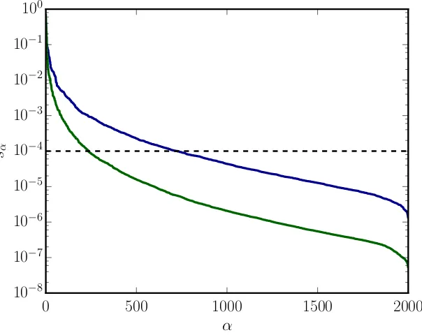
α = sα for sα ≥ t and s0a = 0 for sα < t or by the truncated weight w = Pα>rs2l,α. In
0 500 1000 1500 2000
α
10−8
10−7
10−6
10−5
10−4
10−3
10−2
10−1
100
sα
Figure 2.5: Two singular value distributions (solid lines) and a fictitious truncation threshold
t= 10−4 (black dashed line). The same value oftresults in different errors after the truncation at the bond according to Eq. (2.1.22)since the distribution of singular values is different.
Fig. 2.5 two different distributions of singular values sα can be seen and a line at a
fictitious truncation threshold t= 10−4. The corresponding sum of the discarded squared
values is very different in both cases and without knowing the distribution of the singular values one can not determine how big the corresponding error is after the truncation. However, in most calculations those two truncation measures can roughly be connected byw≈t2. For all our calculations we will denote the amount of truncation in terms of a
truncated weight.
We want to emphasise again the very important connection between the entanglement of a state and the bond dimension needed to describe the state accurately. The stronger entangled a state is, the more non-zero singular values of approximately the same size exist, which does not allow for an efficient truncation and thus leads to a high bond dimension. Matrix product states are only an efficient description for relatively lowly entangled states. Fortunately, it has been shown that for ground states of systems with size L and a gap between the ground state and excitations the entanglement between two halves of the system goes with ∼ LD−1, where D denotes the spatial dimension of
the system. This is known as the area law[73,77] and states for one-dimensional systems
2.2
Matrix Product Operators
It is not only possible to decompose any state|ψi into a product of matrices but also any
operator. These so-called matrix product operators (MPOs) can be constructed in the same fashion as MPSes. Given a Hilbert spaceH=⊗L
lHl and corresponding basis states
{|σli} of the Hilbert spaces Hl we can write any operator ˆH :H → H as
ˆ
H= X
σ1,τ1 X
σ2,τ2
· · · X
σL,τL
cσ1,σ2···σL
τ1,τ2···τL |τ1i ⊗ |τ2i ⊗ · · · ⊗ |τLihσ1| ⊗ hσ2| · · · hσL|. (2.2.1)
Analogously to the decomposition of the multi-dimensional coefficient tensor of the matrix product state in the previous section, we can decompose the coefficient tensor c of the operator ˆH with size Πld2l into a series of tensors {Wwlσl,τl−1,wl} of rank 4
cσ1,σ2···σL
τ1,τ2···τL = X
w1 X
w2
· · ·X
wL
Wσ1,τ1
1,w1 W
σ2,τ2
w1,w2· · ·W
σL,τL
wL−1,wL. (2.2.2)
A graphical representation of an MPO is depicted in Fig. 2.6 as well as an MPO-MPS application in Fig. 2.7. It can be seen that after the contraction of the indices
connect-W5
|τ1i |τ2i |τ3i |τ4i |τ5i |τ6i |τ7i |τ8i |τ9i |τ10i
W2
W1 W3 W4 W6 W7 W8 W9 W10
|σ1i |σ2i |σ3i |σ4i |σ5i |σ6i |σ7i |σ8i |σ9i |σ10i
Figure 2.6: Graphical representation of a matrix product operator. In contrast to an MPS, now we have two local indices, one located on the bottom of each square representing a tensor and one at the top. Again, connecting lines are indicating contractions and are called bonds (as for MPS).
ing the MPO and MPS we will obtain an MPS again. In general, the bond dimension mR
i =wiOm ψ
i of the new MPS tensor of site i will be the product of the bond dimension
of the MPO mO
i and MPS m
ψ
i , which normally will be truncated immediately to some
smaller value ˜wR
i ≤ mRi . Since this is rather inefficient, other approaches like the zip-up
algorithm[80] or a variational approach[43] are recommended. The key idea of the zip-up
algorithm is to contract the tensors of MPS and MPO consecutively and truncating each tensor directly before contracting the next site. This approach has proven to be as accu-rate as the naive contraction of MPS and MPO and significantly faster. The intermediate tensors occurring during the computation only have a bond dimension ofmR
i ×di×wOi m ψ i
with di being the bond dimension of the local state space |σii. In contrast, during the
the naive approach tensors with bond dimensionwO i m
ψ
i ×di×wiO×m ψ
i occur, which are
larger in general.
W5
|σ1i |σ2i |σ3i |σ4i |σ5i |σ6i |σ7i |σ8i |σ9i |σ10i
W2
W1 W3 W4 W6 W7 W8 W9 W10
A1 A2 A3 A4 M5 B6 B7 B8 B9 B10
Figure 2.7: Graphical representation of a multiplication of an MPO to an MPS. After the contraction of the MPO and MPS a new matrix product state is obtained. In general the bond dimension of the new MPS is much higher than of the original MPS.
4.2.1 in the context of orthogonalisation, except that the environment tensor must be replaced by the contraction of the MPS, MPO and current estimate MPS.
Density Matrix Renormalisation
Group
The density matrix renormalisation group (DMRG) was developed by Steve White in 1992[13] for infinite systems and soon became the most powerful numerical method for
studying one-dimensional quantum lattices and determining their ground states[81]. The
key idea is to consider an increasing number of lattice sites and truncating the number of states describing the system to keep the size of the Hilbert space manageable. For that it is assumed that there exists a reduced state space that describes the essential physics of the system effectively and that DMRG can identify this subspace. Later, because of its great success, DMRG was extended to finite systems and systems with long-range cor-relations too. This is achieved by building up a one-dimensional lattice with the desired system size with infinite DMRG and afterwards using iterative sweeps over the system to determine a converged ground state description of the system[43,81].
While DMRG was initially only used to compute ground states and static properties of low-energy spectra of strongly correlated Hamiltonians such as the Heisenberg, Hubbard and t−J model, it was extended to study dynamic properties such as frequency depen-dent conductivities and dynamical structure factors[82,83,84] as well.
As described in the introduction of the previous chapter, in the late 90s the connection between DMRG and matrix product states (MPS) was discovered[64,65], which finally led
to the very effective and adaptive MPS-based formulation of DMRG[45,68]. Nevertheless,
it is still true that two-dimensional systems can only be solved for very small system sizes, while one-dimensional systems are typically solvable with DMRG up to an accu-racy that is only limited by machine precision. There exist several ides how to tackle two-dimensional systems, such as mapping the problem to an one-dimensional system[74]
or using projected entangled pair states[75,76], but all methods have in common that the
required numerical resources increase drastically.
However, research is still ongoing with the aim of improving the performance of DMRG further. This includes the combination of tensor networks with global symmetries[85,86,87]
Chem-istry[21]. This is even more important since model Hamiltonians become more and more
realistic and consequently more complex. In this context, DMRG is also combined with other methods like dynamical mean-field theory which generates Hamiltonians that in-clude long-range interactions between numerous lattice sites, which give rise to small but at the same time very strongly entangled systems. Thus, ideas and methods from other fields such as Quantum Chemistry can lead to huge performance improvements. Most of these methods has been validated in calculations of highly correlated molecules for decades and still have not found their way into the condensed matter community. Some concepts as reordering of lattice sites based on entanglement information[21,89],
variation-ally obtaining better bases sets for the lattice sites[90] or even changing the topology of
the whole lattice system[40,44] are focused on reducing the entanglement in systems and
thus can lower bond dimension of MPSes significantly. Other approaches try to systemat-ically find better starting states based on Hartree-Fock orbitals to reduce the convergence times[88,91] compared to using arbitrary random starting states. Overall, improvements
based on these concepts can very often lead to performance increases by factors up to ten or higher. Therefore, it is not surprising that DMRG is still considered to be a key method for tackling two-dimensional problems for the future.
In this chapter we want to present the fundamental concept of DMRG based on the MPS formalism and several improvements we find useful for the rest of the thesis, This includes the formulation of strictly single-site DMRG as well as the reordering of lattices based on entanglement information. In the end of this chapter we will shortly focus on binary tree tensors, which were developed by us together with collaborators during this thesis. A first implementation showed that they start to be competitive with usual one-dimensional MPSes for system sizes that were slightly larger than necessary for our models. However, other lattice topologies used in quantum chemistry, such as minimal entangled trees or minimal spanned trees, are a promising route to decrease entanglement in systems further and should be kept in mind for further research. Therefore, we will end this chapter by providing a short introduction to these very interesting concepts.
3.1
Single-Site-DMRG
The aim of DMRG is to find the state |ψi represented by a matrix product state which
minimises the energy of a Hamiltonian ˆH, represented as an MPO,
min
|ψi E =
hψ|Hˆ|ψi hψ|ψi
!
. (3.1.1)
We can reformulate the problem to the minimisation ofhψ|Hˆ|ψiunder the constraint that
hψ|ψi= 1. This can be solved using a Lagrangian multiplier[92] λ, resulting in
min
|ψi
Optimising the complete MPS corresponds to solving a highly complex non-linear problem which is nearly impossible to do efficiently and reliably. Instead, the key idea of DMRG is to optimise the tensors of the MPS iteratively one after the other while moving through the system using SVDs. This reduces the problem to a multi-linear optimisation problem which can be solved efficiently via the following trick: We assume the the state|ψiis in the mixed-canonical representation with the tensors on sites 1 to l−1 being left-normalised
and the tensors on sitel+1 toLbeing right-normalised. In the notation of matrix product states we can write the overlap hψ|ψi as
hψ|ψi=X
σl
X
al−1al X
a0
l−1a
0
l
ΨA
al−1,a0l−1M
σl† al−1,alM
σl a0l−1,a0lΨ
B
al,a0l, (3.1.3)
where we kept the tensor of site l explicitly. The tensors on the left and right hand site of site l we combined as
ΨA
al−1,a0l−1 = X
σ1,...,σl−1
(Mσl−1†· · ·Mσ1†Mσ1· · ·Mσl−1)
al−1,a0l−1, (3.1.4)
ΨB al,a0l =
X
σl+1,...,σL
(Mσl+1· · ·MσLMσL†· · ·Mσl+1†)
a0
l,al. (3.1.5)
Because of the chosen representation and the orthogonality properties of the tensors, par-ticularly clear in the graphical representation (Fig. 3.1), the last two expressions simplify to unit matrices
ΨA
al−1,a0l−1 =δal−1,a
0
l−1 and Ψ
B
al,a0l =δal,a0
l. (3.1.6)
Let us now consider the term hψ|Hˆ|ψi, with ˆH written in MPO language
hψ|Hˆ|ψi= X
σl,σ0l
X
a0l−1,a0l
X
al−1,al X
bl−1,bl
Lal−1,a
0
l−1
bl−1 W
σl,σl0 bl−1,blR
al,a0l bl M
σl∗
al−1,alM
σl0
a0l−1,a0l (3.1.7)
withLbeing the contraction of all tensors left of sitelwith the MPO tensors andR equiv-alently defined for the tensors on the right of sitel. In Fig. 3.2 a graphical representation of these to operators can be seen. If we now consider the extremum by differentiating with respect to A† and setting the equation equal to zero, we find
X
σl0
X
a0l−1,a0l
X
bl−a,bl
Lal−1,a
0
l−1
bl−1 W
σl,σl0 bl−1,blR
al,a0l bl M
σl0
a0l−1,a0l−λM σl
a0l−1,a0l = 0, (3.1.8)
which is depicted completely in Fig. 3.2. This is an eigenvalue equation. That can be seen by introducing the matrixHby reshapingH(σlal−1al),(σl0a0l−1a
0
l) =
P
bl−1,blL
al−1,a0l−1
bl−1 W
σl,σ0l bl−1,blR
al,a0l bl
as well as the vector ν with νσlal−1al =M
σl
al−1,al and arriving at
A1 A2 A3 A4 M5 B6 B7 B8 B9 B10
A∗
1 A
∗
2 A
∗
3 A
∗
4 B
∗
10
B∗
9
B∗
8
B∗
7
B∗
6
M∗
5
M5
M∗
5
Figure 3.1: a) Graphical representation of the overlap of a state |ψi with itself. The ket state is depicted on the bottom while the bra state hψ| is on the top. Since the state is written in the mixed canonical representation with respect to site l(= 5), the contractions of the tensors
A and B with their complex conjugated counter parts result in unit matrices, leaving only the contraction of the centre tensor Mσl as seen in b).
with matrix dimension (dm2 ×dm2) for H. Solving for the lowest eigenvalue λ and its
eigenvectorν will result in the locally optimal tensor Mσl
al−1,al after reshapingν. A simple
SVD lets us move to the next site while staying in the mixed canonical representation. We can then optimise the local tensor on sitel+1 by solving another eigenvalue problem. This can be done very efficiently when the operators L and R are saved and updated iteratively instead of calculated completely anew. We can sweep back and forth from the left edge to the right edge of the system in this manner, visiting and updating each site for the lowest eigenvalue until we observe convergence. The eigenvalue solver best suited for DMRG is, depending on details, the Lanczos or the Jacobi-Davidson method since, in general, the matrix dimension ofH dD2 is too large for an exact diagonalisation. Lanczos
only requires the application ofH onto the local tensorAlwith costsO(2m3dw+m2d2w2)
and thus equally much as the contraction of the left and right part of the HamiltonianL and R but significantly more than the SVD O(m3d). It is therefore not surprising that
between 75% and 95% of the total runtime of the single site DMRG algorithm is spent on the eigensolver step. However, the single-site DMRG algorithm is a very easy and cheap way of finding the ground state of a system.
The left and right sweeps are repeated until convergence is achieved which is measured with respect to the energy. Typical values which we want to reach are changes below ∆E <10−10. A much better test is to consider hψ|Hˆ2|ψi −(hψ|Hˆ|ψi)2 to check whether
DMRG found an eigenstate. Therefore, the expression should approach 0 as closely as possible. Unfortunately, for large bond dimension of the Hamiltonian (mH ≈ 16) the
calculation of ˆH2|ψi becomes too demanding, not allowing us to follow this route.
M5
B6 B7 B8 B9 B10
A1 A2 A3 A4
A∗
1 A
∗
2 A
∗
3 A
∗
4 B6∗ B7∗ B8∗ B9∗ B10∗
M5
W1 W2 W3 W4 W5 W6 W7 W8 W9 W10 −λ× = 0
Figure 3.2: Graphical representation of the eigenvalue equation with the definition of the matrices
L and R describing the effective basis of the left and right part of the system.
starting state|ψihas to be parallel to the global ground state to allow DMRG to converge
to it. A significant drawback of single-site DMRG is that the bond dimension during the optimisation procedure cannot be increased but only decreased during the SVDs. If the ground state |E0i has a higher amount of entanglement than the initial state |ψi and
therefore needs a larger bond dimension, it is impossible to obtain a good description of
|E0i. The usual way of solving this issue is to optimise not only a single site but two
adjacent sites at the same time. In the so-called two-site DMRG algorithm, the tensors of site l and l + 1 are combined before and split up after the solution of the eigenvalue problem. The split up with the SVD allows for an increase of the bond dimension of the tensor Ml. However, this increases the size of the effective matrix H and thus slows the
algorithm down significantly.
3.2
Strictly Single-Site DMRG
In 2015 Hubig et al. developed a version of the single site DMRG which optimises a single site tensor with an additional subspace expansion[93]. The subspace expansion
al-lows an increase of the bond dimension and thus improves the convergence properties substantially. This new approach performs DMRG calculation significantly faster since the scaling of single-site DMRG O(m3dw) is better by a factor of d than the scaling of
two-site DMRG O(m3d2w). This improvement is scaled down slightly by the fact that
the single-site DMRG method needs more sweeps to converge.
The idea of a subspace expansion originates from the numerical lineal algebra commu-nity[94,95] and relies on the fact that a matrix product of two matrices A ∈ Rm×n and
B ∈ Rn×p can be expanded with another matrix P in A and zeros in B while keeping
their product A·B ∈Rm×p invariant
A·B →hA Pi·
"
B 0
#
W5
W2
W1 W3 W4
A1 A2 A3 A4 M5
A∗
1 A
∗
2 A
∗
3 A
∗
4
L4
Figure 3.3: Graphical representation of the expansion term defined in Eq. (3.2.4) for a left-to-right sweep after the optimisation of site5. The indices on the left of site 1 and the right of site
iare fused together.
This also can be done in the MPS context. The expansion over the bondml from the left
is written as
Mlσl →M˜lσl =hMlσl P σl l
i
, (3.2.2)
Mσl+1
l+1 →M˜ σl+1
l+1 =
"
Mσl+1
l+1
0
#
. (3.2.3)
With this approach single site DMFT can optimise the sitel+ 1 with the increased bond dimensionml+mPl whereml is the original bond dimension andmPl is the dimension of
the added rows of sitel. If the optimisation finds out that elements of the enlarged space are not lowering the energy they are simply discarded by setting the associated factors on sitel+ 1 to zero.
It is noteworthy that after the expansion, as in standard DMRG, an SVD is used to move to the next site. During the SVD the most relevant statesmr of the enlarged space
ml+mPl are selected. This allows to increase the bond dimension adaptively but can also
lead to original states of the matrixMlσl being discarded. Unless the expansion states are lower in energy, this can increase the energy slightly.
Mathematically, choosing the local components of the exact residual written in MPS notation as the expansion term offers global convergence to the minimum as Dolgov and Kressner showed in their original work[94]. Since this is in general very costly to compute,
Hubig et al.[93] proposed an expansion term of the form
Pl =αLl−1MlWl, (3.2.4)
also depicted in Fig. 3.3. The termMlWl on the l-th site describes the application of the
MPO Wl to the current MPS Ml, while the left-contraction Ll−1 is a projection of the