estimation
Roman Hornung
estimation
Roman Hornung
Dissertation
an der Fakult¨at f¨
ur Mathematik, Informatik und Statistik
der Ludwig–Maximilians–Universit¨at
M¨
unchen
vorgelegt von
Roman Hornung
aus Augsburg
Zweitgutachter: Prof. Dr. David Causeur
Drittgutachter: Dr. Marie-Laure Martin-Magniette
high-dimensional biomedical data play a central role.
The first project is concerned with the question of whether it is necessary to include data preparation steps in cross-validation procedures in situations where such proce-dures are followed to estimate the prediction error of biomedical prediction rules. In practice many data preparation steps are, in most cases, not repeated within cross-validation on the training datasets, but rather performed beforehand on the entire dataset. Thereby, the training data and test data are not entirely separated, which, for some data preparation steps, can lead to a relevant underestimation of the pre-diction error. However, it is mostly unknown for which of these data preparation steps there is a danger of severe underestimation of this kind. In this project, first a general measure is developed to assess the magnitude of this underestimation. Next, this measure is applied to real datasets in extensive analyses in order to determine whether it is necessary to include two data preparation steps—normalization and principal component analysis—in cross-validation procedures.
In the second project an innovative method for batch effect adjustment is developed using which parts of a dataset that are systematically distorted, can be homogenized. This new method differs from others in that it removes both differences in terms of means and variances among the different dataset parts and corresponding differences in terms of the dependence structures of the variables. Using simulated data and real data, the performance of the new method is compared to that of popular alternative methods.
beitung hoch-dimensionaler biomedizinischer Daten eine zentrale Rolle spielen. Das erste Projekt befasst sich mit der Frage nach der Notwendigkeit des Einschlus-ses von Vorverarbeitungsschritten in Kreuzvalidierungsverfahren, wenn letztere zur Sch¨atzung des Vorhersagefehlers von biomedizinischen Pr¨adiktionsregeln verwendet werden. In der Praxis werden viele Vorverarbeitungsschritte zumeist nicht innerhalb der Kreuzvalidierung auf den Trainingsdatens¨atzen wiederholt, sondern vorher auf dem ganzen Datensatz durchgef¨uhrt. F¨ur manche Vorverarbeitungsschritte kann die-ses Vorgehen durch die damit verbundene Aufhebung der vollst¨andigen Trennung von Trainings- und Testdaten zu einer relevanten Untersch¨atzung des Vorhersagefehlers f¨uhren. Es ist jedoch weitestgehend unbekannt, f¨ur welche Vorverarbeitungsschrit-te eine derartige UnVorverarbeitungsschrit-tersch¨atzung zu bef¨urchten ist. Deshalb wird in dieser Arbeit zun¨achst ein allgemeines Maß zur Absch¨atzung des Ausmaßes dieser Untersch¨atzung entwickelt. Dieses Maß wird anschließend in ausf¨uhrlichen Analysen auf echte Da-ten angewendet, um die Frage nach der Notwendigkeit des Einschlusses der beiden Vorverarbeitungsschritte Normalisierung und Hauptkomponentanalyse in Kreuzvali-dierungsverfahren abschließend zu beantworten.
Im zweiten Projekt wird eine innovative Methode zur sogenannten Batcheffektent-fernung entwickelt, anhand derer sich systematisch verzerrte Teile eines Datensatzes homogenisieren lassen. Die Besonderheit der neuen Methode gegen¨uber existieren-den Alternativen besteht darin, dass sie sowohl Unterschiede in existieren-den Mittelwerten und Varianzen zwischen den verschiedenen Teilen des Datensatzes beseitigt als auch entsprechende Unterschiede in der Abh¨angigkeitsstruktur der Variablen. Die Perfor-manz der neuen Methode wird anhand simulierter und echter Daten mit popul¨aren, alternativen Methoden verglichen.
Anne-Laure Boulesteix. She has pointed me in suitable directions and was always available for questions and helpful discussions. Moreover, she created an excellent encouraging collegial atmosphere in which I always felt secure during the preparation of the dissertation.
I would also like to extend my sincere thank to Prof. Dr. David Causeur. During my three research stays in Rennes I always felt very welcome. He pointed me in suitable directions as well, and in our many helpful discussions I was able to gain valuable insights.
Moreover, I am very grateful to my “periodical” colleagues at the Applied Mathe-matics Department at Agrocampus Ouest in Rennes, who amicably took care of me during my research stays in Britanny, for work as well as leisure.
Many thanks also to my colleagues at the Department of Medical Informatics, Biometry and Epidemiology for the great atmosphere.
Last but not least, I would like to thank my parents and my friends for their con-tinued support and encouragement inside and outside of work.
2. Measuring the impact of CV incompleteness with respect to data
prepa-ration steps 13
2.1. Background . . . 13
2.2. Methods . . . 15
2.2.1. Data material . . . 15
2.2.2. Addon procedures . . . 17
2.2.3. (Addon) normalization . . . 18
2.2.4. (Addon) principal component analysis . . . 19
2.2.5. The CV incompleteness impact measure (CVIIM) . . . 19
2.2.6. Global CVIIM . . . 21
2.2.7. Illustration . . . 22
2.2.8. Study design . . . 24
2.3. Results . . . 25
2.3.1. Normalization . . . 25
2.3.2. Principal Component Analysis . . . 26
2.4. Discussion . . . 29
2.4.1. Alternative measures of CV incompleteness . . . 29
2.4.2. Outlook: other preparation steps . . . 30
2.4.3. Simulation study . . . 37
2.4.4. Combination of several steps . . . 38
2.4.5. Further issues . . . 40
2.5. Conclusions . . . 44
3. Combining location-and-scale batch effect adjustment with data clean-ing by latent factor adjustment 45 3.1. Background . . . 45
3.2. Methods . . . 49
3.2.1. Description of existing batch-effect adjustment methods . . . . 49
3.2.2. FAbatch . . . 53
3.2.3. Addon adjustment of independent batches . . . 57
3.2.4. Comparison of FAbatch to other methods . . . 61
3.3. Results . . . 68
3.3.1. Ability to adjust for batch effects . . . 68
3.3.2. Application in cross-batch prediction . . . 75
3.3.3. Artificial increase in measured class signal by applying SVA . 80 3.4. Discussion . . . 82
4. Improving cross-study prediction through addon batch effect
adjust-ment or addon normalization 85
4.1. Background . . . 85
4.2. Methods . . . 88
4.2.1. Data material . . . 88
4.2.2. (Addon) Batch effect adjustment and (addon) quantile normal-ization . . . 88
4.2.3. Cross-study validation . . . 90
4.2.4. Study design . . . 90
4.3. Results . . . 91
4.3.1. Addon quantile normalization . . . 92
4.3.2. Addon batch effect adjustment . . . 93
4.4. Discussion . . . 97
4.4.1. Reasons for no benefit from combining the two approaches . . 97
4.4.2. Random forest: impaired performance in the presence of dif-fering class frequencies between training data and test data . . 98
4.4.3. Boosting as a (potentially) robust method to avoid overfitting in the context of cross-study prediction . . . 99
4.4.4. Further possibilities for application . . . 100
4.5. Conclusions . . . 101
5. Conclusions and outlook 103 A. Appendices to Chapter 2 115 A.1. Simulation study for the example of supervised variable selection . . . 115
A.2. Methodological background . . . 122
A.2.1. Prediction rules, prediction errors, and their estimation . . . . 122
A.2.2. Incomplete opposed to full CV . . . 124
A.2.3. Behavior of CVIIMs,n,K for small εf ull(ntrain,K) values . . . 125
B. Appendices to Chapter 3 127 B.1. Plots used in verification of model assumptions . . . 127
B.2. Target variables of datasets used in comparison study . . . 133
B.3. Reasons for batch effect structures of datasets used in comparison study134 B.4. Boxplots of the metric values for simulated datasets for each method and simulation scenario . . . 135
B.5. Tables showing the means of the metric values and of the corresponding ranks in simulated datasets by method and by scenario . . . 142
The analysis of modern, high-dimensional, biomedical data usually involves special
preliminary data preparation steps, for example normalization or filtering by variance,
which are performed before addressing the questions of thematic interest. With
tra-ditional medical datasets preprocessing usually is more straightforward and easier to
conduct. Preliminary steps in this field may involve standardizing the variables or
im-puting missing variables. Given the increasingly important role of high-dimensional
biomedical data in medical research, data preparation can be expected to gain
atten-tion in the scientific literature.
This thesis consists of three parts, in each of which, preparation of high-dimensional
biomedical data plays a central role. In the first part the impact of excluding specific
data preparation from cross-validation on the estimated error is analyzed with the aid
of the cross-validation incompleteness impact measure (CVIIM) developed specially
for this purpose. In the second part, a new batch-effect adjustment method for high-dimensional data is presented, which, in addition to adjusting for location-and-scale
batch effects, adjusts for batch effects evident in the correlation structures within the
batches. In the third part, a compendium of microarray datasets is used to determine
the extent to which, and under which circumstances, cross-study prediction can be
improved with the aid of addon batch effect adjustment and addon normalization.
Background
In the following, several terms which play a crucial role in the thesis are explained.
High-dimensional data
This term describes datasets featuring more variables than observations.
High-throughput datasets are specific types of high-dimensional datasets featuring many—
often many thousands of—biomolecular variables. In this context, each variable often
However, in the last few decades many methods have been developed that are
special-ized for this data format. Many of these methods were used in the analyses presented in this thesis.
Data preparation step
In general, this term is used for any analysis step performed before conducting
anal-ysis steps that deliver the final result of the study. However, in this thesis there is a difference between data preparation steps performed observation by
observa-tion, such as background correction in microarray data, and data preparation steps
which use information across observations. Examples of the latter steps are quantile
normalization of microarray data, batch effect adjustment (see below), and variable
selection. In this thesis only steps of the second kind are considered, which is why in
the following, the termdata preparation step refers to this kind of data preparation.
Normalization
Various factors influencing raw high-throughput data lead to differences among
obser-vations. Such differences are due to elements beyond the biological signal of interest.
Therefore, the distributions of the raw values generally are made similar across
obser-vations by employing a normalization method. Due to differences among the various
high-throughput data structures, each data type requires the use of a specific
normal-ization method. An important method is the quantile normalnormal-ization method (Bolstad et al.; 2003), which is used in this thesis. After employing this method, the empirical
distributions of the data values are identical across the different observations.
Prediction rule
A central application field of high-throughput data is the prediction of disease states
of patients. To this end, prediction rules are used. A prediction rule is an algorithm
that uses the values of a number of variables in a patient (covariates) to predict the
unknown value of a specific phenotype variable of interest (target variable). Such
prediction rules are obtained, or learned, using the data on a series of patients for
whom the covariate values and the values of the target variable are known. These
data are commonly denoted astraining data. The algorithm that is used for learning
the prediction rule is specific to the latter. This thesis is concerned with prediction
rules for high-dimensional data with binary target variables. A prediction rule of this
applying the classification trees constituting the constructed RF to the data on a new patient and aggregating the results to obtain a prediction of his/her value of the
target variable.
When applying prediction rules in practice one is confronted with the raw covariate data on new patients. Therefore, here, as a preliminary step, any data preparation
steps that have been taken while learning the prediction rule have to be taken for
the data on new patients as well. It is impossible to obtain a prediction based on the
patients’ raw covariate data, because the learning algorithm which delivered the final
prediction rule has used the form of the training data obtained after preparation.
Due to the widespread use of data preparation steps, this issue can be expected to
be equally widespread in practice. However, this issue seems widely overlooked in
the scientific literature. In this thesis the following definition of prediction rules is
given: A prediction rule comprises not only the algorithm specific to the method outputting the predictions based on the preprocessed data, for example the RF, but
also any data preparation steps to be performed before the preprocessed data can be
committed to this algorithm. In accordance with this definition, the algorithm used
for learning such a prediction rule comprises all data preparation steps.
Estimation of the error of a prediction rule
Before applying a prediction rule, it is important to assess how accurately it can
predict the values of the target variable of independent patients. If the error frequency
of a prediction rule is too high, it should not be applied in practice. This is because
doctors and patients would be misinformed too frequently if such a rule were used for
diagnosis. A na¨ıve and very problematic approach to estimate the error frequency
would be the following: Apply the prediction rule to the training data with which it was learned and calculate the frequency of which the prediction rule delivers an
incorrect prediction for this data. It is well-known that this can lead to a severe
underestimation of the error frequency to be expected for independent data. The
reason for this is that the prediction rule tends to be better adjusted to its training
data than to the independent data for which it is intended. Therefore, as a general
rule the data used to estimate the error frequency, the test data, should be different
from those used to learn the prediction rule. Here it is possible to discern two cases: 1)
The test data are distinct from the training data but originate from the same dataset
as the training data, referred to as internal validation; 2) The test data stem from
dataset than that of the training data, external validation results in more realistic
error estimates than internal validation. As data from different datasets other than from where the training data originate, generally behave more differently than those
from the same datasets, external validation results in higher error estimates (see e.g.
Bernau et al. (2014)).
K
-fold cross-validation
The most prominent method for estimating the error frequency to be expected in
internal validation is K-fold cross-validation or short cross-validation (CV). High-throughput datasets are often quite small; therefore, splitting the dataset into training
data and test data usually leads to at least one of the following two problems: 1) The
test dataset is too small to provide an acceptable accuracy of the error estimate; 2)
The training dataset is too small to ascertain a level of prediction performance similar
to that which results when using the entire dataset as a training dataset. K-fold CV addresses these issues first by re-performing the error estimation for different splits
of the entire dataset into training data and test data and second by choosing a large
enough amount of training data. Precisely, K-fold CV is conducted as follows: 1) Split the dataset randomly into K (approximately) equally sized parts, denoted as folds; 2) For k ∈ {1, . . . , K}: estimate the error frequency using fold k as test data and the rest of the dataset as training data; 3) Take the average of the error estimates
from 2). To reduce further the variance of the error estimation, in practice K-fold CV should be repeated multiple times. Although K-fold CV is less variable than error estimates obtained when using single splits into training data and test data, its
variance is still high (Efron and Tibshirani; 1997). Ostensibly, no widely accepted
guidelines exist for choosing the number of foldsK.
Batch effects
Traditional clinical data most often directly mirror the biological phenomena of
in-terest such as age or sex. By contrast, the data values from microarray-based data
types constitute measurements of the respective biological phenomena such as gene
expression. These measurements are unwantedly influenced by external conditions.
There are numerous external factors that can influence microarray data, such as the
laboratory in which the data are produced, the technician treating the data and
even the time of data generation. As a result, data of observations which have the
gen-as abatch. Batch effects lead to limited comparability of data from different sources, which can negatively influence analyses being performed using the combined data.
In contrast to microarray-based data types, which require measuring the underlying
biological phenomena, more modern high-throughput data types such as RNA-Seq
data allow direct investigation of the underlying biological phenomena. Nevertheless,
data collection in the case of these modern high-throughput data types is prone to
error and batch effects have been found to be a problem with these data as well
(Hansen and Irizarry; 2012).
In this thesis, the definition of batch effects comprises not only effects caused by
external conditions of the data generation process but also by differences in data cohorts due to differing study populations, as long as these differences do not affect
the biological phenomena to be studied with the aid of the data.
Batch effect adjustment
Given that batch effects can influence analyses negatively, it is desirable to
re-move such effects beforehand by assimilating the distributions of the data across
the batches. A method with such an aim is called a batch effect adjustment orbatch
effect removal method. A number of such methods exist. Some of them are very
simple, for example, zero-mean centering of the variable values in the batches, while
others are more sophisticated, for example, adjusting for location-and-scale
differ-ences across batches as performed by ComBat (Johnson et al.; 2007). Note that
batch effect adjustment is a data preparation step.
Cross-study prediction
As mentioned above, a prediction rule is applied in practice to data stemming from
entirely different sources than those of the training data. This procedure is referred
Contents
In this section the three projects presented in the thesis are described in order to
provide an initial overview of the work.
Chapter 2: Measuring the impact of CV incompleteness with
respect to data preparation steps
As stated above, in CV the prediction rule is learned repeatedly using different subsets
of the available dataset. The learning process of obtaining a prediction rule also
comprises the data preparation steps involved according to the definition of prediction
rules given above. Therefore, from a formal standpoint, data preparation should be
re-performed using the training data in each iteration of the CV. Performing data
preparation on the entire dataset before performing error estimation is equivalent to learning part of the prediction rule using both training data and test data. This can
have negative implications. Above it was stated that the prediction rule is better
adjusted to the data on which it was learned. If these data comprise the test data for
part of the learning process, as done when performing data preparation on the entire
dataset, it can be expected that the test data are better adjusted to the prediction
rule than truly independent data are. Again, this may lead to underestimation of the
error frequency. Chapter 2 is concerned with the latter phenomenon.
In fact, for various reasons, it is common practice to perform certain data
prepara-tion steps, for example, quantile normalizaprepara-tion, using the entire dataset before CV.
The extent of underestimation of the error frequency resulting from this, that is, the
impact of such anincomplete CV, differs among data preparation steps. Steps mak-ing use of the target variable more frequently are associated with a stronger impact
on the estimated error through incomplete CV. However, as will be shown in the
analyses in Chapter 2, there also are steps which use only the covariate values but
nevertheless should not be performed on the entire dataset before error estimation to
warrant against underestimating the error frequency.
The work presented in Chapter 2 resulted from the following three considerations:
1) The impact of incomplete CV depends on the data preparation step under
consider-ation; 2) It is not clear which data preparation steps have to be performed within CV
to prevent a relevant optimistic bias; 3) Someone confronted with a dataset cannot be
expected to decide for his/her specific analysis whether or not he/she should include
a data preparation step in CV. These considerations necessitate the formulation of
to use a measure of the impact of incomplete CV. In Chapter 2 such a measure is provided with the CV incompleteness impact measure (CVIIM) which depends on
the distribution underlying the dataset used for estimating it. Therefore, in addition
to CVIIM, with the global CVIIM a measure is provided that does not depend on a
specific data distribution. The estimation of this measure requires several datasets.
With the aid of CVIIM and global CVIIM and through using large collections of real high-throughput datasets, guidelines for the following two commonly used data
preparation steps are developed: normalization and principal component analysis
(PCA). These guidelines state that while normalization can be performed beforehand
on the entire dataset, PCA should be included in CV. Corresponding empirically
based guidelines ostensibly were previously available only for the data preparation
step “supervised variable selection”. In addition to the guidelines for normalization
and PCA, preliminary results obtained for other common data preparation steps are
provided.
Chapter 3: Combining location-and-scale batch effect adjustment
with data cleaning by latent factor adjustment
Due to the wide variety of factors leading to batch effects, the latter are equally
diverse in nature. Therefore a batch effect adjustment method intended to work well
for various datasets should do at least one of the following: 1) address coarse types of batch effects that are present in all datasets affected by batch effects. Examples
of methods of this kind are mean-centering, standardization, ratio-A, ratio-G (Luo
et al.; 2010), and ComBat; 2) adjust to the specific kind of batch effects of the dataset
being analyzed. An example of a method of this kind is surrogate variable analysis
(SVA) (Leek and Storey; 2007).
Methods of the first kind may miss important characteristics of batch effects present
in the specific dataset being analyzed, for example, sophisticated dependence
struc-tures induced by batch effects. By contrast, methods of the second kind may miss
simple batch effect structures which can easily be addressed, for example,
mean-differences of the variables across batches. In Chapter 3 a method is presented with
FAbatch that addresses coarse features of batch effects and adjusts to sophisticated
batch effect patterns specific to the individual dataset being studied. FAbatch
repre-sents an extension of ComBat, that is, adjustment for location-and-scale differences of
the variables across batches. With FAbatch, in addition to location-and-scale
within batches, that is, variations in the observations not attributable to the
biolog-ical signal of interest are addressed, which is very similar to the approach followed by SVA. However, in contrast to FAbatch, SVA was developed for situations where
it is not known which observation belongs to which batch. The primary goal of the
adjustment for latent factor influences performed by SVA is to remove
heterogene-ity resulting from observations belonging to different batches. The adjustment for
latent factor influences performed by FAbatch within batches, by contrast, should
capture sophisticated properties of the batches specific to the dataset being studied.
In the estimation of the latent factor models, it is important that the biological
sig-nal of interest be protected. Otherwise, not only unwanted differences among the
observations attributable to batch effects would be removed, but also would desired differences attributable to the biological signal. SVA uses a specific procedure for
protecting the biological signal. This procedure can lead to a dangerous exaggeration
of the biological signal, as will be discussed in detail in Chapter 3. By contrast, with
FAbatch the signal exaggeration is mitigated by using predicted class probabilities
instead of the actual classes in the protection of the biological signal.
In Chapter 3, using a large collection of real high-throughput datasets, FAbatch is
extensively compared to commonly used competitors with respect to several metrics.
These metrics measure either the homogeneity of the data across batches after batch
effect adjustment or the performance of analyses performed using the batch effect
adjusted data. Here, FAbatch proves to be equal to the other methods in many
situations and superior in some situations.
Moreover, for illustrative purposes FAbatch and its competitors are applied in a
prediction context. In prediction, batch effect adjustment can be employed to render
data to which the prediction rule is to be applied more similar to the training data. In
this thesis, reference is made to addon batch effect adjustment when applying batch
effect adjustment in this way. Addon batch effect adjustment is properly defined in
Chapter 3 and will be at the center of Chapter 4.
Chapter 4: Improving cross-study prediction through addon batch
effect adjustment or addon normalization
When obtaining prediction rules, it is implicitly assumed that the data to which the
rule is intended to be applied follow the same distribution as that underlying the
training data. However, this assumption is—due to batch effects—not given in many
cases when applying prediction rules in practice. Consequently, the true error of a
a way that they follow the same distribution as the training data. In the following the termtest datawill be used for the data to which a prediction rule is applied. Note
that this term also is used for the data used to estimate the error rate of a prediction
rule. However, there is no likelihood of confusion between the two meanings because
the correct meaning of this term will be clear from the respective context.
As noted above, batch effect adjustment can be performed to transform the test data in order to adjust them to the training data. Many batch effect adjustment
methods can be applied to this end without the need for alteration. Others have to
be adjusted in such a way that the training data are not changed in the process of
considering varying test datasets. However, the latter is not a difficult task using
the general blueprint for determining the addon procedure for a specific batch effect
adjustment method introduced in Chapter 3.
The aim of batch effect adjustment is to assimilate the distributions of the
individ-ual variables across different data subparts. The aim of normalization is quite similar:
to adjust the marginal distributions of the data values across observations. Thus,
nor-malization also can be used in adjusting the test data to the training data. Here, as
with batch effect adjustment, it has to be warranted that the training data are not
altered when transforming the test data. A normalization procedure that fulfills this
is termed addon normalization in the following. The only difference between a
nor-malization procedure and an addon nornor-malization procedure is the following: In an
addon normalization procedure, those parameters involved which are not observation-specific are estimated using the training data only, sparing out the test data. The
addon normalization procedure for robust multi-array average (RMA) normalization
was developed by Kostka and Spang (2008). Addon procedures can be determined for
any data preparation steps that involve considering information across observations
(see Chapter 2).
From an intuitive point of view, it is clear that both addon batch effect
adjust-ment and addon normalization should lead to better prediction results when the test
data follow a different distribution from that of the training data before adjustment.
However, in Chapter 4 a large study of real data is conducted to investigate the value
of these procedures in a prediction context for the following two main reasons: 1)
Even though an improvement is expected, it is not clear whether there is indeed a
notable gain in prediction performance by applying these procedures in practice; 2)
There are various batch effect adjustment methods and it is not clear whether all of
them lead to an improvement. In this extensive study 25 real microarray datasets are
test sets.
From the results of this extensive study of real data the following conclusions can
be drawn: 1) There is an improvement both by addon batch effect adjustment and
addon normalization; 2) Addon batch effect adjustment generally is more effective
than addon normalization; 3) There is no advantage of combining addon batch effect
adjustment and addon normalization over using addon batch effect adjustment alone;
4) While addon batch effect adjustment is recommendable in principle, it should be applied only when the test datasets are not too small and when the distribution of
the target variable is similar in training data and test data; 5) Only those batch effect
adjustment methods that address coarse batch effects seem to be appropriate. Other
kinds of methods impaired performance in the analyses.
Publications and submitted articles
The works described in Chapters 2, 3, and 4 have been published in the journals
BMC Medical Research Methodology, BMC Bioinformatics, and Bioinformatics,
re-spectively:
• Hornung, R., Bernau, C., Truntzer, C., Wilson, R., Stadler, T., and Boulesteix, A.-L. (2015). A measure of the impact of CV incompleteness on prediction
error estimation with application to PCA and normalization. BMC Medical
Research Methodology, 15, 95.
• Hornung, R., Boulesteix, A.-L., and Causeur, D. (2016). Combining location-and-scale batch effect adjustment with data cleaning by latent factor
adjust-ment. BMC Bioinformatics, 17, 27.
• Hornung, R., Causeur, D., Bernau, C., and Boulesteix, A.-L. (2016). Improving cross-study prediction through addon batch effect adjustment or addon
normal-ization. Bioinformatics, doi: 10.1093/bioinformatics/btw650.
Moreover, the R package bapred was developed in the context of the project
pre-sented in Chapter 3. This package allows batch effect adjustment and addon batch
effect adjustment using the new method FAbatch and various other common batch
effect adjustment methods. Further, it provides various metrics for assessing the
success of batch effect adjustment. The package was extended in the context of the
Chapters 1 and 5 were written by me without any contributions by others. Moreover,
I was the main contributor of the manuscripts of the papers underlying Chapters 2
to 4.
I wrote, by far, the greatest part of the manuscript of the paper underlying Chapter
2. The co-authors helped with revising the manuscript, setting up the study design
of the empirical study presented in section 2.2.8 and implementing the simulation
study presented in Appendix A.1 and in section 2.4.3.
The manuscript of the paper underlying Chapter 3 was written also almost com-pletely by me. The co-authors helped with revising the manuscript, setting up the
design of the empirical comparison study presented in section 3.2.4 and contributed
to the concept of the FAbatch method.
I also wrote the manuscript of the paper underlying Chapter 4 almost completely
by myself. The co-authors helped with revising the manuscript.
With the exception of the help I received in implementing the simulation study for
the manuscript of the paper underlying Chapter 2, I performed all analyses presented
data preparation steps
2.1. Background
In supervised statistical learning, it is widely recognized that prediction models should not be constructed and evaluated using the same dataset. While the training dataset
is used for all steps towards obtaining the prediction rule, the test dataset is used to
evaluate its prediction error and, ideally, should not be at all involved in the training
phase. CV and related procedures involve considering several divisions into training
data and test data and averaging the estimated prediction errors of the respective
prediction rules constructed in each iteration (see also Chapter 1). In this chapter
K-fold CV is used, but all ideas and procedures can be extended to other resampling techniques used for prediction error estimation.
In the following the term incomplete CV (Simon et al.; 2003) refers to CV
proce-dures in which some analysis steps are performed beforehand using the entire dataset.
With incomplete CV, at each iteration the excluded fold acting as test data may af-fect the prediction rule derived, since it was used preliminarily for data preparation
which contradicts the principle of test data requiring perfect separation (Daumer
et al.; 2008). In contrast, if all steps leading to the prediction rules are performed in
each CV iteration using only the corresponding training set, the CV procedure is full
CV.
The problems resulting from incomplete CV have been studied extensively with
regard to preliminary variable selection for classification based on high-dimensional
microarray data (Simon et al.; 2003; Ambroise and McLachlan; 2002; Wood et al.;
2007; Zhu et al.; 2008). If performed before splitting the dataset intoK folds, super-vised variable selection often leads to strongly, downwardly biased error estimates.
(Si-mon et al.; 2003; Ambroise and McLachlan; 2002), that is, considering it part of the
classifier construction process. Similarly, it has been suggested that parameter tuning should be performed using the training dataset only (Varma and Simon; 2006; Bernau
et al.; 2013; Boulesteix and Strobl; 2009). However, the bias resulting from incomplete
CV with respect to parameter tuning ostensibly has never been investigated.
Variable selection and parameter tuning are—by far—not the only procedures of-ten performed in practice before CV. For example, raw data from high-throughput
biological experiments such as microarrays have to be normalized before high-level
analyses such as predictive modeling can be conducted. The selection of features
ex-hibiting considerable variability across the observations is another example of a data
preparation step often performed when analyzing microarray data. Further examples
relevant to any type of data include imputation of missing values, dichotomization,
and non-linear transformations of the features. Preparation steps are not limited to
these few examples. The analysis of increasingly complex biomedical data (including,
e.g., imaging or sequencing data) requires the use of evermore sophisticated prepro-cessing steps for making raw data analyzable. Note again that the question of the
impact of CV incompleteness is not relevant to those steps which prepare the
obser-vations independently of each other, such as background correction for microarray
data.
Although it is known that incomplete CV is problematic in the case of variable
selection, it is unknown which other preparation steps lead to underestimation of
the prediction error if performed before splitting the dataset into K folds. To date there seems to be no consensus on whether it is necessary to include all steps in CV:
Some authors postulate that all steps are required to be included (Westerhuis et al.;
2008), which seems to be done rarely, regardless; others only suggest this procedure
for variable selection (Ambroise and McLachlan; 2002) or, generally, for supervised
steps (Hastie et al.; 2009).
Some practical problems which deter researchers from performing full CV include
the computational effort often needed to repeat time-intensive preparation steps, the
fact that some preparation steps such as variable selection are sometimes conducted
“in the lab” before the data are given to the statistician (Zhu et al.; 2006), and the
lack of (user-friendly) implementations of addon procedures allowing the adequate preparation of the excluded fold when the preparation step has been conducted
us-ing the trainus-ing folds only (see section 2.2.2 for more details on addon procedures).
Another practical problem occurs in the context of genotype calling in genetic
asso-ciation studies: It is common practice to use not only the entire dataset of interest,
but also additional datasets to improve genotype calling accuracy.
PCA and normalization—for example normalization using the RMA method (Irizarry et al.; 2003) for microarray gene expression data. It is not clear whether the prediction
error estimate that results is optimistically biased if one applies these two methods
to the entire dataset before splitting the data intoK folds. In an effort to answer this question, a measure is presented in this chapter which enables the quantification of
the impact of incomplete CV with regard to steps of interest, theCV incompleteness
impact measure (CVIIM). It is based on the ratio of the CV prediction error which
results when the preparation steps investigated are applied only once using the entire
dataset to the CV prediction error which results when they are incorporated into
CV. The latter means that, within CV, in addition to performing the investigated preparation steps on each training dataset anew they are applied to the excluded fold
through addon procedures.
The goal of this chapter is two-fold: (i) to present the new measure CVIIM, which is
intended to be used by methodology researchers or statisticians working on statistical learning applications to determine whether a particular preparation step should, in
general, be trained in each CV iteration successively or whether it can be performed
safely as a preliminary step on the entire dataset without generating a relevant
opti-mistic bias; and (ii) to apply this new measure to answer this question for two
impor-tant preparation steps, PCA and normalization, in order to provide corresponding
guidelines for these steps.
This chapter is structured as follows: In section 2.2 first the microarray gene
ex-pression datasets used in the empirical studies described below, the concept of addon
procedures, and the two methods, normalization and PCA, are presented. Then
CVIIM is introduced and its use and behavior in the well investigated case of
vari-able selection are briefly illustrated using four datasets. Finally, the designs of the
studies on the impact of CV incompleteness with respect to normalization and PCA
are described. In section 2.3 the results of these studies are presented. In section
2.4 preliminary results obtained for other data preparation steps are presented and further issues are discussed. In section 2.5 the main conclusions drawn from this
chapter are summarized.
2.2. Methods
2.2.1. Data material
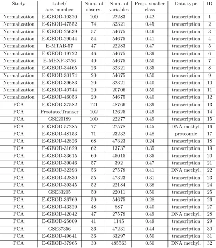
Study Label/ Num. of Num. of Prop. smaller Data type ID
acc. number observ. variables class
Normalization E-GEOD-10320 100 22283 0.42 transcription 1
Normalization E-GEOD-47552 74 32321 0.45 transcription 2
Normalization E-GEOD-25639 57 54675 0.46 transcription 3
Normalization E-GEOD-29044 54 54675 0.41 transcription 4
Normalization E-MTAB-57 47 22283 0.47 transcription 5
Normalization E-GEOD-19722 46 54675 0.39 transcription 6
Normalization E-MEXP-3756 40 54675 0.50 transcription 7
Normalization E-GEOD-34465 26 32321 0.35 transcription 8
Normalization E-GEOD-30174 20 54675 0.50 transcription 9
Normalization E-GEOD-39683 20 32321 0.40 transcription 10
Normalization E-GEOD-40744 20 20706 0.50 transcription 11
Normalization E-GEOD-46053 20 54675 0.40 transcription 12
PCA E-GEOD-37582 121 48766 0.39 transcription 13
PCA ProstatecTranscr 102 12625 0.49 transcription 14
PCA GSE20189 100 22277 0.49 transcription 15
PCA E-GEOD-57285 77 27578 0.45 DNA methyl. 16
PCA E-GEOD-48153 71 23232 0.48 proteomic 17
PCA E-GEOD-42826 68 47323 0.24 transcription 18
PCA E-GEOD-31629 62 13737 0.35 transcription 19
PCA E-GEOD-33615 60 45015 0.35 transcription 20
PCA E-GEOD-39046 57 392 0.47 transcription 21
PCA E-GEOD-32393 56 27578 0.41 DNA methyl. 22
PCA E-GEOD-42830 55 47323 0.31 transcription 23
PCA E-GEOD-39345 52 22184 0.38 transcription 24
PCA GSE33205 50 22011 0.50 transcription 25
PCA E-GEOD-36769 50 54675 0.28 transcription 26
PCA E-GEOD-43329 48 887 0.40 transcription 27
PCA E-GEOD-42042 47 27578 0.49 DNA methyl. 28
PCA E-GEOD-25609 41 1145 0.49 transcription 29
PCA GSE37356 36 47231 0.44 transcription 30
PCA E-GEOD-49641 36 33297 0.50 transcription 31
PCA E-GEOD-37965 30 485563 0.50 DNA methyl. 32
ArrayExpress database (www.ebi.ac.uk/arrayexpress) (Kolesnikov et al.; 2015) or the NCBI GEO database (www.ncbi.nlm.nih.gov/geo) (Barrett et al.; 2013). All datasets feature a binary target variable and are of human origin. Details
on the biological background of the datasets may be obtained online with the
re-spective accession numbers available in Table 2.1 and via the R scripts written
for the preparation of the individual datasets for analysis. The latter are
avail-able athttp://www.ibe.med.uni-muenchen.de/organisation/mitarbeiter/070_ drittmittel/hornung/cviim_suppfiles/index.htmland can be used to download and prepare the individual datasets automatically. The dataset ProstatecTranscr
appeared in Singh et al. (2002) and is available in the form of anRda-file at the above link as well. Here, R scripts also are provided for reproducing all analyses presented
in this chapter.
In the search for suitable datasets those which featured a strong class imbalance or
would have been difficult to handle from a computational point of view were excluded.
2.2.2. Addon procedures
In this section a brief overview is given of the concept of addon procedures. When
a data preparation step has been conducted on the training data only, the test data
must be prepared equivalently: To not do so might render the test data nonsensical
with regard to, or even incompatible with, the prediction rule derived from the
train-ing data. A na¨ıve but straightforward procedure in the case of steps which do not
involve the response variable (unsupervised steps) such as normalization (see section
2.2.3) is to prepare the test data completely independently, that is, without using any information from the preparation of the training data. For the prediction of
exter-nal data such a separate data preparation procedure may be suitable for some steps
when the external data behave very differently from the training data: By separate
processing the data preparation procedure can adjust itself to the peculiarities of the
external data (see e.g. Bin et al. (2014)). However, in many situations this approach
may lead to greater prediction error particularly in the case of small test datasets
due to the larger variance of the output of preparation steps. Test datasets of size
one (corresponding to, for example, patients examined one at a time) are an extreme
case in which this approach is even unfeasible. Moreover, for some preparation steps
such as variable filtering by variance this na¨ıve approach cannot be applied because it would lead to the selection of different variables in the training datasets and test
datasets and thus make the application of the prediction rule impossible.
data and to use the output of the preparation step to prepare the test data. In the
following, this is referred to as an addon procedure. This term originally was intro-duced in the specific case of normalization for microarray data (Kostka and Spang;
2008) but is employed here for all types of data preparation steps. In this thesis, the
following definition is used: An addon procedure for a data preparation step prepares
an observation in the test data precisely as it would prepare a corresponding
obser-vation in the training data, where, however, the parameter estimates involved have
been obtained exclusively on the training data. This, of course, excludes parameters
specific to the individual observations. These parameters are still estimated using
the data of the corresponding observations. Note that by performing a preliminary
step the following is meant in the context of this chapter: 1) Conduct the preparation step on the data considered; 2) Store all information necessary for addon preparation
of new observations. Addon procedures are trivial in some cases, for instance, that
for dichotomization according to cutpoints determined from the training data (one
simply uses the training-data-derived cutpoint to dichotomize the test data) or that
of variable selection (selecting precisely those variables in the test data which were
selected based on the training data). However, in other cases, such as normalization
of microarray data or imputation of missing values, this task is more complex.
2.2.3. (Addon) normalization
Normalization of microarray data essentially is the transformation of the data in such
a way as to eliminate or reduce systematic differences among observations unrelated
to biological differences. In this chapter two methods of microarray data
normaliza-tion are considered: 1) RMA and 2) RMA where the quantile-normalizanormaliza-tion step is
expanded by variance stabilization normalization (VSN) (Huber et al.; 2002)
with-out calibration (RMAglobalVSN) (Huber; 2014). RMA consists of three steps: 1) background correction, 2) quantile normalization (Bolstad et al.; 2003), and 3)
sum-marization. Background correction and summarization are performed on an
array-by-array basis, which is why no addon strategies are necessary for these procedures. The
quantile normalization step is performed conceptionally as follows: Letxsort,i∗j be the
j-th smallest variable value of array i∗. Then for each array i ∈ {1, . . . , n} the j-th smallest value is determined and the average ¯xsort,j over thesenvalues taken. Finally xsort,i∗j is replaced by ¯xsort,j. By performing this procedure for all variable values, the empirical distributions of all arrays become equal. When normalizing the test
obser-vations using addon quantile normalization (Kostka and Spang; 2008) the averages of
out the latter having been changed during the procedure. VSN transforms the gene expression values in such a way that the variance of the differences between values
of different observations is rather constant across the entire intensity range. In the
vignette of the Bioconductor package vsn, Huber (2014) presents a version of VSN in which no calibration is performed, that is, only a global variance stabilization
transformation is conducted. In contrast to standard VSN this procedure does not
involve any observation-specific parameters, so it is possible to determine an addon
procedure: The global VSN parameters estimated on the training data are used to
transform the test data.
2.2.4. (Addon) principal component analysis
PCA is an unsupervised dimension reduction method commonly used in the
con-text of high-dimensional data analysis. The principal components are calculated
using a singular value decomposition (SVD) of the centered data matrix. The
ad-don procedure is as follows: 1) Center the values of each variable by subtracting
the corresponding variable mean estimated from the training data; 2) Multiply the
matrix resulting from 1) by the PCA loading matrix derived from the training data to obtain the principal components. The principal components with highest variance
can be viewed as a summary of the data in fewer dimensions and often are used in
practice for graphical representation of the data. In the context of classification using
high-dimensional data, it is common to fit a prediction rule with a prediction method
such as discriminant analysis using principal components as predictors instead of the
original variables (Dai et al.; 2006).
2.2.5. The CV incompleteness impact measure (CVIIM)
In the following, CVIIM, the new measure to determine the extent of bias induced
by incomplete CV with respect to a data preparation step of interest, is presented.
Let s be the available dataset from which a prediction rule is to be derived. s is
assumed to be ani.i.d.sample of sizenwith observations drawn from the distribution
P, where P is the joint distribution of predictors and a response variable. Note that the assumption of i.i.d. observations made here is owing to the fact that this
chapter is concerned with CV, that is, dataset internal validation. With external
based on the training dataset only. Similarly, leteincompl,K(s) be the prediction error estimated by incomplete K-fold CV, that is, the data preparation step(s) of interest is/are performed before CV, using the entire dataset. For simplicity of notation, it
is assumed that ef ull,K(s) and eincompl,K(s) are obtained by averaging over a large
number of CV runs, that is, over a large number of random partitions, and can thus
be treated as deterministic.
For S ∼Pn, the measure CVIIM is defined as:
CVIIMP,n,K :=
1 − E[eincompl,K(S)]
E[ef ull,K(S)]
if E[eincompl,K(S)] < E[ef ull,K(S)]
and E[ef ull,K(S)] > 0
0 otherwise.
(2.1)
Note that CVIIMP,n,K is defined as a theoretical quantity, not calculable, but
possible to estimate from real data. It is estimated simply by replacing the expected
CV errors with their empirical counterpartseincompl,K(s) and ef ull,K(s):
CVIIMs,n,K :=
1 − eincompl,K(s)
ef ull,K(s)
if eincompl,K(s) < ef ull,K(s) and ef ull,K(s) > 0
0 otherwise.
(2.2)
Clearly, CVIIMP,n,K ∈[0,1]. The same holds for the estimator CVIIMs,n,K. CVIIM
is based on the ratio of the incomplete CV error to the full CV error, which is more
revealing than their difference as a measure of the impact of CV incompleteness.
Indeed, the latter would depend heavily on the value of the error (large error values
leading to large differences), as suggested by the results shown in section 2.4.1 and
by the simulation presented in section 2.4.3 and in Appendix A.1. Truncation at
zero prevents CVIIM from being negative in the unlikely case that the incomplete
CV error is larger than the full CV error. A large value of CVIIM indicates that CV
incompleteness results in a large underestimation of the prediction error.
The discrepancy betweeneincompl,K(s) andef ull,K(s) depends on the extent to which
the specific preliminary step conducted on the entire dataset increases the
homogene-ity of the covariate values across observations and (for supervised preparation steps) the empirical association between the covariate values and the values of the target
variable.
The interpretation of CVIIMs,n,K and results from real data together with
of CV incompleteness with regard to the considered step(s): [0,0.02] ∼ no impact, ]0.02,0.1]∼ weak, ]0.1,0.2]∼ medium, ]0.2,0.4]∼strong, ]0.4,1]∼ very strong.
In the following an artificial example is outlined to demonstrate, step by step,
a possible application of CVIIMP,n,K. The interest lies in measuring the extent of
overoptimism connected with performing the quantile normalization step of RMA
before CV in gene-expression-based classification. Suppose there is a dataset with
gene expression measurements from 32 patients suffering from breast cancer and from
22 disease-free patients. For each patient there are measurements of the expression
of 54675 genes. As a classification method the nearest shrunken centroids (NSC) are
used (Tibshirani et al.; 2002). The error eincompl,5(s), as estimated by incomplete 5-fold CV, is computed by conducting RMA normalization beforehand on the entire dataset and performing 5-fold CV on the normalized dataset. In this procedure only
the fitting of NSC is repeated in each CV iteration on the training datasets. The
CV is repeated 300 times to obtain more stable results. The full CV error ef ull,5(s)
is computed by performing a 5-fold CV in which the quantile normalization step of
RMA (as well as the fitting of the NSC) is re-performed in each CV iteration on
the respective training set, with addon normalization of the corresponding test set
through the addon procedure by Kostka and Spang (2008). This procedure is repeated
another 300 times. Ifeincompl,5(s) = 0.15 and ef ull,5(s) = 0.1503 were obtained, then
CVIIMs,n,K = 1−0.15/0.1503 ∼ 0.002. According to the aforementioned rules of
thumb this would indicate no impact on the estimated error.
This result obtained for a specific dataset and specific classifier, may not be
rep-resentative of all datasets and classifiers in the field of gene-expression-based
classi-fication. It is necessary to study several datasets and several analysis settings
rep-resentative of the considered field in order to formulate recommendations regarding
incomplete CV for a particular step. Alternatively, specific guidelines could be
for-mulated for particular settings and data types within the considered field; however,
this could result in overly complicated guidelines.
For a detailed formal introduction to the concepts presented in this section such
as prediction rules, prediction error, and its estimation via full and incomplete CV,
consult Appendices A.2.1 and A.2.2.
2.2.6. Global CVIIM
Clearly, the value of CVIIMs,n,K depends on the specific dataset. For a general
the quantity resulting when replacing E[eincompl,K(S)] and E[ef ull,K(S)] in Eq. (2.1) by quantities very similar to their means over the universe of datasets from the area of interest (see Boulesteix et al. (2015) for a more formal description of this concept
in another context). Consider the following example: At this time the standard
ap-proach to microarray data analysis is to perform quantile normalization of RMA on
the entire dataset before performing CV. Suppose that the prediction error is, on
average, 0.2 over all datasets from the area of interest, but if full CV were performed
with respect to quantile normalization it would equal 0.201. The global CVIIM in
this scenario would be 1−0.2/0.201∼0.005, a negligible overall bias.
To estimate the global CVIIM the plug-in estimator can be used, which functions
by replacing eincompl,K(s) andef ull,K(s) in Eq. (2.2) with the averages of their values
obtained for several datasets from the considered area of application:
CVIIMglobals(1),...,s(L);K :=
1 −
1 L
PL
l=1eincompl,K(s (l))
1 L
PL
l=1ef ull,K(s(l))
if L1 PL
l=1eincompl,K(s(l)) < 1
L
PL
l=1ef ull,K(s (l))
and L1 PL
l=1ef ull,K(s
(l)) > 0
0 otherwise,
(2.3)
where s(1), . . . ,s(L) are the datasets used. Note that this estimator is not affected
considerably by individual extreme CVIIM estimates, which can occur in the case of
very small values of E[ef ull,K(S)]. For a detailed discussion on this phenomenon, see
Appendix A.2.3.
2.2.7. Illustration
To give a preliminary illustration of the application of CVIIM as a proof of concept, it
was applied to supervised variable selection, which was expected to yield high CVIIM
values. The following datasets were used: ProstatecTranscr, GSE33205,GSE20189, and GSE37356. These also were considered in the PCA study; see Table 2.1.
For each variable a two-sample t-test was conducted to test the equality of the
means of the two groups. The variables with the smallest p-values were selected.
Because the result was expected to depend substantially on the number of selected
of the variables, LDA could not be applied because the empirical covariance matrices involved are not well behaved in general when the number of variables is higher than
the number of observations. In this case, diagonal linear discriminant analysis was
used, that is, LDA under the simplifying assumption that within the two classes the
variables are independent; see Hastie et al. (2009).
In all the analyses performed in this chapter, eincompl,K(s) and ef ull,K(s) were ob-tained by averaging the results from B = 300 runs of K-fold CV, whereK takes the values 3, 5, and 10 successively.
14 14 14
25
25
25
15 15
15
30 30 30
14
14 14
25 25 25
15 15
15
30 30 30
14 14
14
25
25
25
15 15 15
30
30 30
14 14 14
25
25 25
15 15 15
30 30 30
psel = 5 psel = 10
psel = 20 psel = p/2
0.00 0.25 0.50 0.75 1.00
0.00 0.25 0.50 0.75 1.00
K = 3 K = 5 K = 10 K = 3 K = 5 K = 10
C
V
II
Ms
,n,K
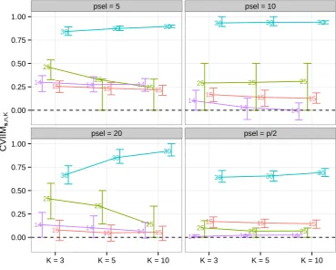
Figure 2.1.: CVIIMs,n,K values from variable selection study. The numbers distinguish
the datasets. psel denotes the number of selected variables.
The CVIIMs,n,K values obtained for all settings are displayed in Figure 2.1. In the
plots the error bars represent the 25% and 75% quartiles (computed over the B = 300 iterations) of the iterationwise non-truncated incompleteness measure estimates
(INIMEs) CVIIMs,n,K,b := 1−eincompl,K(s)b/ef ull,K(s)b, where the index b indicates
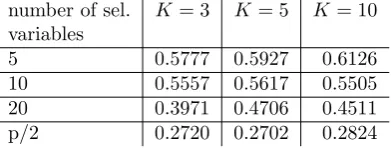
number of sel. K= 3 K= 5 K= 10 variables
5 0.5777 0.5927 0.6126
10 0.5557 0.5617 0.5505
20 0.3971 0.4706 0.4511
p/2 0.2720 0.2702 0.2824
Table 2.2.: Estimates of global CVIIM from variable selection study
the unboundedness of the INIMEs, the error bars—as opposed to the CVIIMs,n,K
values—are not bound by zero.
While CVIIMs,n,K is especially large for small numbers of selected variables,
rel-atively large values also are observed when half of the variables are selected (with
the exception of the dataset with the fewest variables). Although the differences in CVIIMs,n,K for the selection of 5, 10, and 20 variables are not large, the estimates
of the global CVIIM given in Table 2.2 indicate that the bias induced by incomplete
CV tends to decrease with an increasing number of selected variables.
Dataset 30 stands out through its noticeably larger CVIIMs,n,K values in all plots.
This dataset comprises only 36 observations but 47231 variables (see Table 2.1), which
at least may explain in part the larger values. Extreme values above 0.9, however, are surprising.
In this illustrative analysis, employing the new measure CVIIM the following
con-clusion previously obtained in the literature could be confirmed: Performing
super-vised variable selection before CV leads to a strong bias of the resulting error estimate.
2.2.8. Study design
The investigation of normalization is based on the first 12 microarray datasets listed
in Table 2.1. Here, the two variants of normalization described in section 2.2.3
were used. Two classification methods were employed successively to derive
pre-diction rules: NSC and LDA performed on partial least squares components
(PLS-LDA)(Boulesteix; 2004). For NSC the shrinkage intensity ∆ was chosen from the grid {0.05,0.1,0.25,0.5,1,1.5} and for PLS-LDA the number of components ncomp
was chosen from the grid {1,2, . . . ,10}. Parameter choice was done in the following way. For each considered training dataset, 3-fold internal CV was performed for each
candidate parameter value from the grid. The candidate parameter value yielding
the smallest 3-fold CV error was selected.
The study of PCA is based on the last 20 microarray datasets listed in Table
from the grid {1,2,3,5,10}. Since the results can be assumed to depend heavily on the number of principal components used as predictors, the analyses were repeated
for four numbers: 2, 5, 10, and 15.
2.3. Results
2.3.1. Normalization
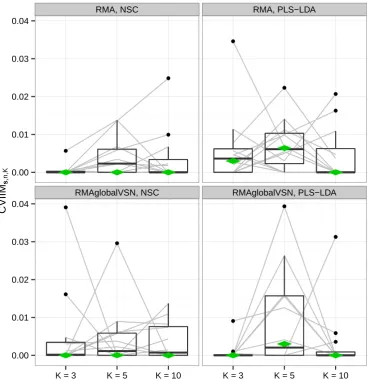
Figure 2.2 depicts the CVIIMs,n,K values from the normalization study together with
the estimates of global CVIIM. The latter are given in Table 2.3.
●
● ●
●
● ●
●
●
●
● ●
●
●
●
●
●
● ●
●
●
● ● ●
●
● ● ●
● ● ●
●
● ● ●
RMA, NSC RMA, PLS−LDA
RMAglobalVSN, NSC RMAglobalVSN, PLS−LDA
0.00 0.01 0.02 0.03 0.04
0.00 0.01 0.02 0.03 0.04
K = 3 K = 5 K = 10 K = 3 K = 5 K = 10
C
V
II
Ms
,n,K
Figure 2.2.: CVIIMs,n,K values from normalization study. The grey lines connect the
Normalization Classification K= 3 K= 5 K= 10
method method
RMA NSC 0.0000 0.0000 0.0000
PLS-LDA 0.0030 0.0064 0.0000
RMAglobalVSN NSC 0.0000 <0.0001 0.0000
PLS-LDA 0.0000 0.0030 0.0000
Table 2.3.: Estimates of global CVIIM from the normalization study
For both normalization approaches the CVIIMs,n,K values are very small for all
datasets and both classifiers. In the majority of cases the measure estimates suggest
no bias resulting from incomplete CV for normalization as defined by the rules of
thumb given on page 21. The global CVIIM estimates seem to confirm that in
general there is no bias. Slightly higher values are obtained for PLS-LDA than for
NSC, but the difference is not noteworthy.
For the individual datasets there is no visible dependence of the measure estimates onK, although in general a negative dependence is expected; see section 2.4.5 for a discussion on this topic. The fact that such a decrease withK is not observed for nor-malization likely can be explained by the small values of the estimates: eincompl,K(s)
andef ull,K(s) are very similar here. Therefore, the non-systematic fluctuations across
the different K values are attributable to small—probably random—fluctuations of
eincompl,K(s) and ef ull,K(s) over K, which could overshadow a potential dependence
onK.
In contrast to section 2.2.7, no iteration-based error bars for the individual CVIIMs,n,K
values are presented here. When depicting the results of a study with a larger number
of datasets, individual error bars make the corresponding plots increasingly unclear.
In this situation it is possible to focus on the distribution of the CVIIMs,n,K values
across datasets; the results for individual datasets are less important. Nevertheless,
extreme individual results should be examined more closely.
Given the small CVIIM estimates it can be concluded that RMA and
RMAglob-alVSN can be performed safely before CV without the danger of inducing a relevant
bias in the resulting error estimate.
2.3.2. Principal Component Analysis
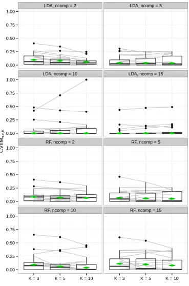
Figure 2.3 and Table 2.4 show the results of the PCA study. Note that the scale
of Figure 2.3 is much larger than that of the corresponding plot for normalization
(Figure 2.2). Globally, the results suggest a weak but existing underestimation of
LDA 2 0.0974 0.0805 0.0582
5 0.0397 0.0371 0.0354
10 0.0000 0.0000 0.0000
15 0.0000 0.0000 0.0000
RF 2 0.0855 0.0747 0.0659
5 0.0686 0.0558 0.0516
10 0.0907 0.0613 0.0368
15 0.1117 0.0988 0.0794
Table 2.4.: Estimates of global CVIIM from the PCA study
values of the global CVIIM estimates are obtained.
For LDA the impact of incomplete CV seems to diminish with an increasing number
of components in PCA. The global CVIIM estimates generally are larger for RF than
for LDA. While the overall effects of performing PCA before CV seem to be weak,
Figure 2.3 reveals that there are several settings in which the CVIIM estimates suggest
a strong bias, according to the rules of thumb given on page 21, for a non-neglible
number of datasets. Therefore, these results strongly favor the use of full CV over
incomplete CV with respect to PCA.
A closer look at Table 2.4 reveals that, in general, the global CVIIM estimates
decrease with an increasing value of K (for all settings with non-zero values). For example, this decrease is noticeable for LDA with ncomp= 2 and RF withncomp= 10. This suggests that the estimates of global CVIIM are overly high in these cases
due to the greater upward bias of ef ull,K(s) compared to eincompl,K(s) as detailed in
section 2.4.5. The global CVIIM estimates depend on the means of the ef ull,K(s)
and theeincompl,K(s) values calculated over the included datasets. The decrease with
larger values of K is induced by the mean of the ef ull,K(s) values becoming more
similar to the mean of the eincompl,K(s) values with increasing value of K. For most settings there is no substantial decrease in the global CVIIM estimates. This suggests
that the two cases for which the decrease withK was strong are connected to aberrant results for individual datasets, which was confirmed by inspecting more closely the
individual values obtained for each setting and each dataset.
More precisely, a simple type of sensitivity analysis was performed. First, for each
of the two settings that dataset displaying the largest difference between ef ull,3(s)
and ef ull,10(s) was omitted and the global CVIIM values were re-estimated. For the
●
● ●
● ● ●
● ●
● ●
● ● ● ● ● ●
●
● ●
●
● ●
●
● ●
● ●
●
● ●
●
●
● ● ●
●
● ● ●
●
● ● ●
● ●
● ●
●
● ● ●
●
● ● ●
●
● ●
● ●
●
●
● ●
●
●
●
● ●
● ● ●
●
●
● ●
● ●
●
● ●
●
LDA, ncomp = 2 LDA, ncomp = 5
LDA, ncomp = 10 LDA, ncomp = 15
RF, ncomp = 2 RF, ncomp = 5
RF, ncomp = 10 RF, ncomp = 15
0.00 0.25 0.50 0.75 1.00
0.00 0.25 0.50 0.75 1.00
0.00 0.25 0.50 0.75 1.00
0.00 0.25 0.50 0.75 1.00
K = 3 K = 5 K = 10 K = 3 K = 5 K = 10
C
V
II
Ms
,n,K
Figure 2.3.: CVIIMs,n,K values from PCA study. The grey lines connect the values