EFFECTS OF A TIME-DEPENDENT MODEL OF GENOTYPIC VALUE ON THE COVARIANCE BETWEEN RELATIVES, VARIANCE COMPONENTS AND ESTIMATES OF HERITABILITY

(1)

EFFECTS OF A TIME-DEF'ENDENT MODEL

O F

GENOTYPIC VALUE ON

THE

COVARIANCE BETWEEN RELATIVES, VARIANCE

COMPONENTS AND ESTIMATES O F HERITABILITY

*

ROBERT F. COSTANTINO

Department of Biology, Genetics Section, Pennsylvania State University, University Park, Pa. 16802

Received February 3, 1969

a recent paper ( COSTANTINO 1968a) the author extended the classical con- 'Yept of genotypic value to include developmental time and suggested that time is an integral part of population dynamics and is therefore a vital part of population analysis. The objective of this communication is to probe further the concept of developmental time by considering ( 1 ) the genotypic covariance between relatives, (2) the components of variance, and (3) heritability estimation. Each of these factors is an important part of quantitative genetic theory and both the manner and magnitude of change in these parameters as a result of developmental time are critical to our understanding of the genetic properties of populations.

TWO LOCUS, T I M E - D E P E N D E N T MODEL O F GENOTYPIC V A L U E

Larval growth, as measured by larval weight, may be empirically idealized by the deterministic model

In w, = In k,

+

c,t

+

(In kz)cit

where In w , is the genotypic value of individual

i

at time t and is composed of the terms, In ki, a non-time value and crt, a time-dependent value. The time- independent value (In

ki)

is determined by locus

K

with alleles e and f; the time- dependent value (c,) is determined by locus

C

with alleles g and h. We are considering a random-mating, equilibrium population in which the two loci combine at random; consequently, the covariance of genotypic values is zero. This is an important point and we shall refer to it later.

The genotypic value In wi may be further partitioned as follows:

* Paper No. 3499 in the journal series of the Pennsylvania Agricultural Experiment Stahon

(2)

522 R. F. COSTANTINO

dKet Wet.. - - Ke

-

Kt C , t =

w . g

- p

= dominance effect of genotype e-f

= additive effect of allele g at time t

= dominance deviations of genotype g-h at time t

= additive X ladditive interaction effect between alleles e and g at time t = additive X dominance interaction effect between allele e and geno-

dCght =

w..&

- p Cgt - cht

( K C )

egt zz W e . g . - p - K e - Cgt

( K d C ) e,ght = We g h - - Ke - Cgt

-

Cht - d'ght

-

( K C ) e g t - ( K C ) eht

type g-h at time t

(dKdC)ef,ght = W e f g h - P - Ke - Kt - dK,rt - Cgt

-

e.. - (CdK)h,eft

= dominance x dominance interaction effect between genotype e-f

The total genotypic variance for In UI, = W e f g h may be expressed symbolically

and genotype g-h at time t .

as

U; = U;

+

UZt'

+

a y

where U:

,

U',

,

U: and U; are the additive and dominance variances with respect

to loci

K

and C, respectively; U:*, U& and uhD are the additive

x

additive, additive X dominance, and dominance X dominance interaction variances and t is developmental time.

k k c C

GENOTYPIC COVARIANCE BETWEEN RELATIVES

The genotypic covariance between relatives follows directly from the paradigm of genotypic value and is

cov( w 1 ,

w,;

t ) = 2r (U;

+

U; t')

+

U(.;

+

U; t')

k C k C

+

[ ( 2 r ) 'U:,

+

2ruuiD

+

u'u&,] t2

.

The genotypic covariance now depends on ( 1 ) r = Malkot's coefficient de parent&, U = probability of

W ,

and W , possessing identical-by-descent geno-

types, (2) the additive, dominance and interaction variances and (3) develop- mental time ( t ) . Each of these terms is a non-negative number, therefore,

d cov (Wl, W 2 ; t ) / d t 2 0 for (all t.

COMPONENTS O F VARIANCE

(3)

TIME-DEPENDENT GENOTYPIC VALUES 523

the hierarchical design of experiment, readers are referred to KEMPTHORNE

( 195 7) and FALCONER ( 1960).

The interpretation of the male ( uL; )

,

female (U;. ) and progeny (U; ) compo-

nents of variance are summarized in Table 1 . It should be noted that the classical and time-dependent models of genotypic value yield identical components with

t = 1. However, with the added dimension of developmental time it is now pos- sible to examine the change in population structure, i.e. the magnitude of change in the variance components, within a generation interval. The following observations are of interest: ( 1 ) the total genotypic variance and its components are a function of developmental time, ( 2 ) the derivative of each of the variance components is positive, consequently, the variances are strictly monotonic increasing functions of developmental time, ( 3 ) the magnitude of change of each of the components differs, for example, epistatic variation influences U;, U;, U; and

uif

in decending order of magnitude.

HERITABILITY ESTIMATION

The heritability of a trait is a n important and useful characteristic for plant and animal breeders for it associates breeding value with phenotypic value and thus leads to the expected or predicted response of a population to selection. The hierarchical design permits three estimates of heritability: ( 1 ) from the male component, (2) from the female component and ( 3 ) U&+ U; yielding an estimate

from full sibs. Each of these estimates is given in Table 2 together with its derivative with respect to developmental time. The male component is nearly identical to the ideal estimate heritability [ ( U 2

+

U; t z ) / u ; ] except for t2 and is

thus the "best" estimate. The full-sib estimate followed by the estimate from the female component are next in order; however, both of these tend to set upper limits to the heritability. Now let us focus attention on the change in these parameters during development. If the epistatic variation is negligible ( U," = 0) then

( 1 ) the heritability from the female component ( h i ) is stable or independent of time, ( 2 ) the heritability from the full-sib component (h;, ) unlike

hi

is still a function of time, and ( 3 ) the heritability from the male component

( h k )

is also a function of time but dh',/dt = 2dh&/dt. Summarizing, the rank order of these estimates with respect to the magnitude of change during development is exmtly opposite to the order based on how closely they approximate the definition of heritability. I t should also be emphasized that the magnitude and direction of change in the h: and h;, and the heritability from offspring-parent (h:,) are dependent on the term ( u ~ , u ~ ~ - - u2 ~~ ) t / ~ : and thus they may increase, de-

crease or remain constant during development even though the components of

variance are strictly increasing functions of time.

(4)

524 R. F. COSTANTINO

4

. .

u U

m

+ ? +

N

N 4 ' NdU N < O

u N U N Y

$2 $2 $2

v v v

. . .

V V N

4 4 4

(5)

TIME-DEPENDENT GENOTYPIC VALUES 525

Table 2

Heritability estimates from male, female, and full s i b components of variance and their derivatives for a Wo-locus time-dependent model of genotypic value.

source Heritability

(c2)

Derivative of i? with respect CO t

Male

Full Sib [U2 W; t2+1/2(U2 WE t2)+

4 , c Dk c

0;

/

(1/2u~+1/40;a+i/8u~~) t21

EXPERIMENTAL OBSERVATIONS

As a means of further elucidating and integrating the properties of the time- dependent model of genotypic value and quantitative parameters, the following experimental observations on a large, random-mating population (Purdue Foun- dation) of Tribolium castaneum were collected. The hierarchical design of experiment consisted of ten randomly chosen males each mated to three females. Four progeny were weighed for each male-female combination at 7, 9, 11 and 13 days of age. The experiment was replicated for a total of 960 observations. Larvae were maintained individually in glass creamers on standard (95

%

wheat flour and

5%

yeast) medium and cultured at 33°C and 52% relative humidity. The weights were recorded in pg and transformed to the natural logarithmic scale.

Before proceeding to the analyses, comment must be made concerning the theoretical model and the experimental data. Recall that larval growth was repre- sented by the deterministic model

In wi =

In

ki

+

c,t

+

(In

ki)c,t

and that the values In

k,

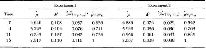
and cL were assumed to be controlled by loci K and C, respectively. The two-locus model wa5 used as a means of conveniently extending the concept of developmental time to the covariance between relatives, variance components and estimates of heritability. With regard to the experimental observations, the values In k , and c, are thought to represent two systems or components of the metric trait, larval weight, each of which may be controlled by many genes but whose effect can be summarized by these two numerical values. It was originally planned to pool the two experiments; however, close exami- nation of the data revealed a fundamental difference in the two studies. As seen in Table 3, the means were approximately linear functions of time and agreed with the theoretical expectations. On the other hand, the total variance was es-

(6)

526 R. F. COSTANTINO

TABLE 3

Mean, variance, covariance and correlation of larval weight (In w ) during development

Experiment 1 Experiment 2

7 4.616 0.108 0.057 0.526 4.889 0.074 0.029 0.542 9 5.723 0.104 0.076 0.711 5.938 0.056 0.036 0.763 11 6.735 0.127 0.087 0.734 6.956 0.061 0.041 0.839 13 7.517 0.110 0.110 1 7.657 0.039 0.039 1

* i = 7,9, 11, 13 days.

ever, the total variance decreased during development in Experiment 2. In the latter case then, as the mean increased, the total variance decreased-refuting the adage that if the mean increases the variance does also. The variance may be expressed as a function of the mean (assuming (In k L ) c Z t = 0) namely,

cT ( p w ) = ( c e / ~ ~ c ) ~ p ~ + 2[cov(ln

k,

c)/pLc - p k c : / ~ : l p w

+

a t p i / p : - 2 cov (In

k,

c) pk/pC +U;

.

In addition to its use as a criterion to stablize the variance during development (COSTANTINO 1968b), the function reveals that if the cov(1n k,c) = 0 the mini-

mum value occurs at the point (pk, U : ) or when t = 0 and thus predicts that as pw

increases so also does U ; . However, if the covariance between the genotypic values

In

k

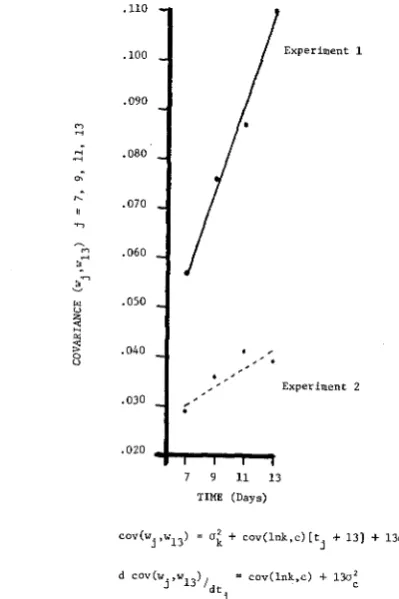
and c is not zero then no a priori association exists between the mean and total variance; hence, although the mean is an increasing function, the variance may increase, remain constant or decrease as was observed in Experiment 2.

Also given in Table 3 is the phenotypic covariance, cov ( w l , wI3), and correlation, pw, wI3, of larval weight at days 7, 9, 11 and 13 with the day 13 weights. Assuming that the interaction term, (In k,)c,t, is negligible, the covariance is a linear function of time and this was observed in both experiments as noted in Figure 1. However. the rate of change in the covariance for Experiment 1 was greater than that for Experiment 2 so that the term (In k:c) f 1 3 ~ : was of differ- ent orders of magnitude. This information, together with the behavior of the total variance, indicates that in Experiment 2 the cov (In k,c) may not be zero, a situa- tion which is not accounted for in classical quantitative genetics (KEMPTHORNE

1957). The correlations in both experiments were similar and as COSTANTINO

( 1968a) showed, are not influenced by the sign of cov (In k,c)

.

The components of variance, additive variance and heritability estimates during larval development for both experiments are listed in Table

4.

You recall from Table 1 that U " , U : , U;. and U', are strictly monotonic increasing functions of time.

(7)

T I M E - D E P E N D E N T G E N O T Y P I C VALUES ₅₂₇ .llO .loo .090 .080 .070 .060 .050 .040 .030 .020

7 9 11 13 TIME (Days)

cov(wj ,w13) =

o i

+ cov(lnk,c) [t .t 131 + 13o't.

d cov(w. ,, w 13),dt

-

cov(lnk,c) + 13of

j C l

FIGURE 1.-Phenotypic covariance of larval weight at days 7, 9, 11 and 13 with 13-day larval weight.

TABLE 4

Components of variance, additive uariance and heritability estimates for

larval weight during development

Experiment 1

Statistic 7 9 11

Total variance ( PT) 0.1079 0.1044 Components:

Progeny

( e P p )

0.1145 0.0985 Female (CZF) -0.0102 0.0068 Male ( 8 Z M ) 0.0038 -0.0009

Additive variance:

Male (&*A,) 0.0153 -0.0036 Female

(e2*,)

-0.0408 0.0272 Full sib (&ZAPS) -0.0128 0.0118

Male (hZM) 0.1415 -0.0345 Female (hZp) -0.3781 0.2773 Full sib (h&) -0.1186 0.1137 Heritability: 0.1272 0.1217 0.0055 0.0002 0.0008 0.0220 0.0114 0.0061 0.1726 0.0936

Experiment 2

13 7 9 11

0.1102 0.0741 0.0561 0.0609

0.0896 0.0574 0.0457 0.0406 0.0091 0.0096 0.0030 0.0122 0.0114 0.0071 0.0074 0.0081

0.0456 0.0284 0.0296 0.0324

0.0364 0.0384 0.0120 0.0488

0.0410 0.0334 0.0208 0.0406

0.4147 0.3833 0.5276 0.5320 0.3369 0.5182 0.2139 0.8013 0.3720 0.4607 0.3707 0.6667

(8)

528 R . F. COSTANTINO

consistently increased, and the female component fluctuated with no clear trend. The estimates of additive variances reflect, of course, the same time change as the components of variance on which they are based.

The heritability estimated from the male component increased during development which is consistent with the model. No clear pattern of change in h i is ap- parent from these data.

The estimate of heritability from the full-sib component is a combination of the male and female estimate and reflects this pattern of change. If one views the days as separate entities then i n Experiment 2, for example, on days 9 and 13 the G.",

>

6; suggesting that there cannot be much nonadditive genetic variance. Thus the two estimates,

R:,

and

RZ,,

may be regarded as equally reliable and their combination, the

h:,

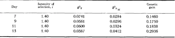
taken as the best estimate. However, on days 7 and 11 this argument can be reversed and the h i , not considered the best estimate. It is the writer's opinion that one should seek general patterns of change in these parameters, and not view them as separate entities, in order to better understand population structure as a dynamic, ever-changing relationship among individuals.

The expected genetic gain has been computed for Experiment 2 from the male estimate of heritability and the results are summarized in Table

5.

The selection intensity is constant, the total variance decreases and the additive genetic variance increases during development. Thus the maximum expected genetic gain occurs

at day 13 when the total variance is minimum.

If one considers the expected genetic gain as

a G = h 2 S = (U: +U: t 2 ) [ u 2 , + u ~ t 2 + 2 C o v ( l n k , c ) t ] - ~ i

where i, the selection intensity, is a constant and cov(1n k,c) is not zero as suggested in Experiment 2 then

dAG/dt =;[mi t ( 2 ~ , + U;

+

U; t 2

+

U; t') - U; U; t

k c

c k k c C C C

+

(3,; t2 - ) C O V ( ~

k,

C ) ] / U ;

.

C k

Thus the magnitude of genetic gain is a function of the components of variance,

TABLE 5

Expected genetic gain as a function of developmental time f o r Experiment 2

Intensity of Genetic

Day selection, i CY211 S'* 1I gain

7 1.40 0.0741 0.0284 0.1460

9 1.40 0.0561 0.0296 0.1750

11 1.40 0.0609 0.0324 0.1838

(9)

TIME-DEPENDENT GENOTYPIC VALUES 529

the intensity of selection, developmental time and the covariance between the genotypic values. The latter is generally assumed zero but nonrandom gene combination can result in equilibrium populations (see LI 1967 for recent review) and will, as noted in this equation for genetic gain, alter the interpretation of population dynamics.

The foregoing experimental data were presented in preference to a numerical example and were meant to focus attention on quantitative measurements and developmental time. The theoretical model analyzed in this study expressed the genotypic values as linear functions of time. However, the functions of the vari- ous genotypes may be of any type (linear, quadratic, exponential, etc.) in time corresponding to the biological basis of the measured variable.

The primary objective of this paper is to add the dimension of developmental time to quantitative genetic analysis. An important aspect of this objective is that quantitative theory is now more accessible to rigorous experimental verification. A theory based on time-dependent genotypic values predicts the magnitude and direction of parametric changes which, as the preliminary data on Tribolium have shown, lends itself to testing procedures.

The writer wishes t o thank Dr. A. A. DEWEES for his critical reading of the manuscript.

SUMMARY

The dimension of developmental time has been added to the interpretation olf the genotypic covariance between relatives. components of variance and heritability estimation. The interpretation of each of these quantitative measurements is affected by time. It is suggested that population structure be viewed as a dynamic continuum and that general patterns of parametric change indicative of that structure be sought using time-dependent models olf genotypic values.

LITERATURE CITED

COSTANTINO, ROBERT F., 1968 (a) The genetical structure of populations and developmental 1968(b) A criterion of transformation for age-weight time. Genetics 60: 409-418. __

data on insect larval growth. Growth 22: 71-73.

FALCONER, D. S., 1960 KEMPTHORNE, O., 1957

LI, C. C., 1967

Introduction to Quantitative Genetics. Ronald Press, N.Y.

An Introduction to Genetic Statistics. Wiley, N.Y.