THEORY OF THE ALLELISM BETWEEN DROSOPHILA LETHALS COLLECTED AT DIFFERENT TIMES

LETHALS COLLECTED A T DIFFERENT TIMES TIMOTHY PROUT

Department of Life Sciences, University of California, Riverside, California 92502

Received February 20, 1967

N a recent paper WALLACE (1966a) presented a n analysis of the allelism of

I

recessive lethal genes in certain population of Drosophila mehogaster. His specific concern was the allelism rates of lethals taken from a natural population at collection sites of varying distances apart. WALLACE argues that the allelism between two sets of lethals from a given distance apart can be related to the allelism of two sets of lethals taken from the same point in the population but separated by a given interval in time.

In connection with this latter relationship WALLACE further conjectures that the allelism rate iTt and the time interval t (in generation units) between the sampling of the first and second sets of lethals have the following functional relationship:

where

iTt = in

+

i , , ( l - K ) t ( 1

1

i T t E the allelism between lethal genes t generations apart

it,

=

the allelism component of iTt within a generation produced by identity by descent in a finite population

i ,

=

the allelism within a generation of the same set of lethal loci if they were in a population of infinite size

K

=

a constant described by WALLACE as “related to the rate of turnover of lethals within the population”.

Note: The lower case

“i”

used here to denote gene allelism is comparable to the upper case

“I”

of WALLACE and of CROW and TEMIN (1964) which denotes chromosome allelism.

It is the purpose of this article to demonstrate that this functional relationship (equation 1 ) conjectured by WALLACE is approximately correct. Furthermore, as a n outcome of this demonstration the parameter

K

will be defined in terms of the basic population parameters of selection and mutation.

One of the important approximations necessary for the derivation that follows is that for all of the lethal loci the change in lethal gene frequency, Aq between successive generations is a linear function of the gene frequency, q in the first of the two generations. This approximation will be assumed to be true at first for the purposes of the derivation and then the approximation itself will be examined. Linear Aq approximation: The relationship between the lethal gene frequencies at a given locus between successive generations may be expressed:

660

where

q

=

gene frequency at generation 0

q1 gene frequency at generation 1

Aq changes in gene frequency due to systematic effects

Sq

=

change in gene frequency due to chance alone. Assume that Aq is a linear function of q as follows:

where Aq

= k(4-q) ( 3 )

k

=

a constant

4

=

the equilibrium gene frequency which should be achieved due to the systematic effects impinging in that locus.

Substituting ( 3 ) into (2) gives

This is a linear recurrence equation whose general term can easily found to be where

.

41 = q

+

k(4-q)

+

sq.

qt = 4-(4-q) ( 1 4 )

+

sqt (4)

t

=

the tth term in the series or in this case number of generations from the start

Sqt

=

the accumulated effects of chance over t generations.

Derivation: Consider the frequency of the lethal allele at a given locus among all lethal alleles at all loci in generation 0. This is a probability, p , which can be expressed as a function of the lethal allele frequency, q, in the whole population (as opposed to among lethal alleles only) and n, the number of loci involved, thus where q

same locus t generations hence

It is assumed the population is in equilibrium and that therefore

4

is constant over this interval of t generations.

The probability of choosing one and the same lethal from among lethals of generation 0 and from among lethals of generation tis p p t ; and

P = q/% = q/nq

the mean lethal allele frequency over all loci. Note: p f 1 - q.

The same probability can be similarly expressed for the lethal allele at the

Pt = q t / ~

This is the probability of allelism at a given locus between the two generations. The total probability of allelism over all loci, or just plain allelism, iTt is substituting

( 5 )

Since, generally speaking,

2

xi = n E ( x ) iTt = z p p t

iTt = ( z q q t ) / ( n 4 ) 2 .

i=n

i=l

nq2 iTt = E ( q q t )

.

stages. First, it is necessary to find the conditional expectation for all those loci sharing one given equilibrium value Q. Then the expectation will be taken over all $.

I t is at this point that it is necessary to introduce the assumption of linear Aq expressed by equation 4. Substituting this expression, equation

4,

for qt in equa- tion 6A and recognizing the conditional expectation, we have

E(qqtj$) = E(qC$ - (q-4) (1-kIt

+

% I )

= E ( q 4 ) - E(q4[1-k]t

+

E ( @ [ l - k ] 7

+

E ( q S q t )

E(qSqt) = E ( q )

E ( % ) .

E(q8qt) = E ( q ) E(Sqt) = E ( q ) (0) = 0 '

(7)

(7A)

Consider the last term first. Since q and Sqt are uncorrelated

The chance deviations 6 q t have expectation of zero so that

Now consider the first term of (7A). Since the population is in equilibrium the expectation of the q's is their common equilibrium value, Q.

E(qQ) =

Applying this relationship and the fact that E ( @ ) = $

+

uq2, equation 6A reduces

to:

E(qqtI$) =

6'

+

uq2( l - k )

where uZq

=

variance of allele frequencies, q, around their mean which is Q.

The variance here is strictly due to the effects of chance since we are dealing with a set of loci subject to exactly the same systematic effects and thus having a common equilibrium, $.

It now remains to take the expectation over all such sets.

E ( q q t ) = E ( @ ' )

+

E(aq2[l-klt)

== 7 2

+

uq2

+

U'( l-K) (8)

where u'=E(uq')

K =

E ( k )

.

u 2

=

variance in equilibriumvalues due to real differences in systematic effects Another assumption has been made above that oq2 and

k

are not strongly corre- lated.

The final expression for allelism,

i~~

can now be constructed by substituting (8) forE(qq,) intoequation 6A.

IT$ =

-

( Q Z + u q 2 + u ' [ 1 - - K ] t )

I.r"

1 u*z u2

- -- + y + y - ( l - I q t

n nq2 nq2 (9)

DOBZHANSKY and HOVANITZ (1942). As these authors pointed out, the first two terms

(-

+

9)represent the theoretical expectation for the allelism of these

same loci in an infinite population. The first factor of the third term

(z)

represents the added increment of allelism due to chance effects or random drift produced by restriction of population (or neighborhood) size. Thus it is seen that the functional relationship, equation 1, conjectured by WALLACE is correct assum- ing the linear Aq relationship. The parameters of WALLACE'S equation therefore have the following more fundamental and usual (WRIGHT, DOBZHANSKY and

HOVANITZ)

interpretation:

1 u 2

n n?

.9"

U 2

l p =

--=-

nq2

(10)

.

1 Uq2

zn=-+-

n nq2

K = E ( k ) , i.e. the mean

k

over all loci expressing, as seen in equation 3, the intensity at which individual genes are driven back each generation towards their equilibrium values by systematic effects alone.

The assumption of linear Aq: It now remains to examine the assumption that

Aq is linear and to find a more fundamental interpretation of K . The exact expression for Aq for a given lethal allele is:

. -

where ,p

=

mutation to the lethal allele from the normal allele, and s 3 selection coefficient of heterozygotes.

The equilibrium,

q,

given by ( 11 ) is

$ = -s(l,+p) f \ / ~ ~ ( l + f i ) ~ -t 4p(1-2~) 2 (1 - 2s)

(The sign of the root is given by the sign of s.)

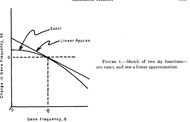
The graphical relationship between the exact Aq and the linear approximation is sketched in Figure 1. As indicated

in

the sketch the linear approximation is

arranged so as to be tangent to the exact Aq curve at the point Q = $.

This procedure implies that the expected equilibrium in a finite population is that given by (12), while WRIGHT (1937) has shown that for a complete recessive ( s = 0), the expected equilibrium is somewhat depressed by the in-

breeding in a small population. It is believed that this discrepancy will not account for large errors in the argument which follows.

As indicated by equation 3, the slope of the linear approximation is -K, which can now be evaluated in terms of the parameters s and p of the expression for the exact Aq (equation 11 ) in the following way:

K = - I Q d A q d q

- s (l.+,p)

+

2g ( 1-2s)

-

m

a

0 C

al

0 C

.-

al

M

c

m

r

0

FIGURE 1.-Sketch of two A 9 functions- one exact, and one a linear approximation.

\-

I

I

I

I

I

I

G e n e F r e q u e n c y , q

Substituting (12) for

4,

approximating the denominator of (13) by unity, and dropping second order terms gives

K

= d s 2 i- 4p approximately. (14)

(The sign of the root is given by the sign of s.) Thus

WALLACE’S

K can now be interpreted in the more fundamental terms of the selection and mutation affect- ing the lethals under study. K can be further simplified if it be assumed that most of the lethals are semidominant, or most are completely recessive, or most are heterotic. Under these three circumstances K simplifies in the following way:

( A ) Most loci semidominant, s positive and

>

>

p

K

= s approximately

(B)

Most loci completely recessive, s = 0

.

K = 2 VTapproximately

(C) Most loci heterotic, s negative and -s

>

>

p

K = -s approximately

Unfortunately, estimates of

K

derived from data appropriate to this model will not decide between the important question of average semidominance or average heterosis, i.e. K is always positive so that the sign of s is ambiguous. Only if K

turned out to be of the order of twice the square root of ordinary mutation rates, then one could conclude that neither semidominance nor heterosis prevailed. A correction for the linear approximation: Referring to Figure 1 it can be seen that the value of Aq given by the linear approximation will be nearly correct only for those loci whose alleles are close to their equilibrium values, $. For those genes which are some distance on either side of the equilibrium, the linear approxi- mation gives a Aq which is always too large compared to the exact Aq.

Restricting the case to allelism between successive generations, E(qql) may be rewritten:

W q q d = Eq(q

+

4 )

= f E(q A).

If under the linear approximation, Aq is always too large then E(qAq) is too

large and so

i

should fall off faster

with increasing t than the theoretical equation 9 predicts. A correction in equation 9 which would cause it to decrease faster with increasing t would be one which reduces the size of the factor (1 - K ) . An approximate correction of this sort may be obtained by replacing (1 - K ) in equation (9) with (1 - K

-

4)

t. This was found by the writer to be entirely satisfactory for a few numerical cases.

It should be noted that the magnitude of the correction increases with increas- ing q. This is so because the linear approximation to Aq progressively deteriorates as one passes from a situation in which most loci are semidominant ( s =

1/)

through recessivity ( s = 0) to heterosis ( s is negative). Also the average equi-

librium,

4

increases through this sequence.

Thus the correction suggested above becomes more important as the linear approximation to Aq deteriorates.

is too large. This means that the actual

i

T t T t

DISCUSSION

It should be emphasized that the above considerations apply only to WALLACE’S coni ecture concerning the functional relationship between allelism and time (equation 1 ) . On the other hand, WALLACE’S data deal strictly with allelism of lethals sampled at one point in time but at different distances apart. WALLACE further proposes, on the basis of his studies of dispersal (WALLACE 1966b), that this same functional relationship (equation 1) can be applied to his data with the substitution of the square root of distance for time. For the rationale for this interesting additional proposal the reader is referred to WALLACE’S paper. It should suffice to point out here, that although the distance-allelism data fit a function of the form of equation 1 and serve well for an estimate of WALLACE’S “zero point allelism”, it is not possible to estimate K since there is an unknown constant of proportionality connecting time with the square root of distance. It

is clear that this distance-allelism relationship, already put to good use by WALLACE, still requires additional theoretical and experimental study.

However, this should not detract from the fact that the time-allelism relation- ship proposed by WALLACE and which is the subject this article is a new and potentially powerful tool for further analysis of Drosophila population structure. The experiments which this theory calls for are straight forward, although laborious. One needs only to sample lethals from a population at different times and perform very extensive allelism tests within and between such samples.

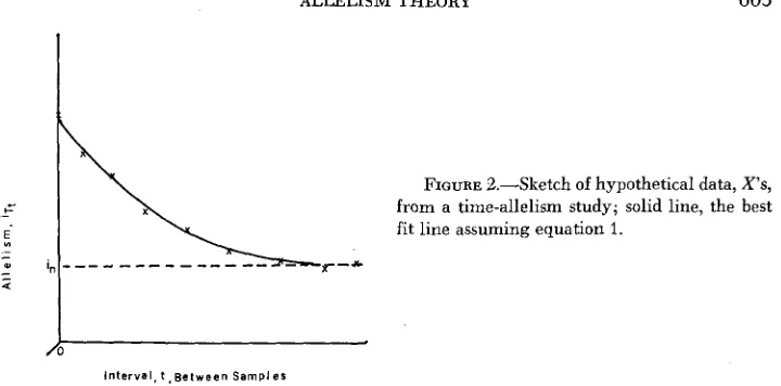
FIGURE &.--Sketch of hypothetical data, X s ,

from a time-allelism study; solid line, the best fit line assuming equation 1.

*-*

-

4

/

I n t e r v a l , t , ~ e t w e e n S a m p l e s

the other hand, a good fit would open up a number of other possibilities. Estimates of the constants,

i,

and

iF

could be set equal to their expectations shown by equa- tions (1 0). Also the same could be done with the constant, K (equation 14). With these, plus the information on lethal frequencies and mutation rates it would be possible to obtain information about all five of the fundamental parameters n,

U(?, 2, s and p on a single population as it exists through time. Heretofore, for a given small population it has not been possible to estimate

i,,

the allelism of that population’s lethal loci if it were of infinite size. Without this time-allelism information in the past, it has been necessary to compare small experimental populations with large ones (PROUT 1954) assuming the populations were the same except for size, or in studies of natural populations (WRIGHT, DOBZHANSKY and HOVANITZ 1942;

PAVAN

and KNAPF 1954)

in

is obtained from allelism be- tween remote localities i n which case the assumption must be made that all the localities are the same.

Finally, even more information should emerge from the simultaneous use of both the time-allelism and distance-allelism tools on a given wide-spread natura1 population. More theoretical work is needed here not only on the distance- allelism relationship, but also on the time-allelism relationship since the con- siderations of this article apply only to strictly isolated populations. Nevertheless, it is conceivable that with the use of both tools one could obtain information on natural generation time and neighborhood size.

SUMMARY

WALLACE (1 966a) has conjectured that recessive lethals extracted from Dro- sophila populations at different times will exhibit decreasing rates of allelism, iTt,

the greater the time interval t between samples, according to the functional

relationship due to

identity by descent in the finite population,

in

=

the allelism shown by the same loci if the population were of infinite size, and K

=

a constant described by

WALLACE

as “related to the rate of turnover of lethals

within

the population”.-

i

= i,

4-

iF

(1 - K ) t , where

iF

=

the component of

i

666

A proof is provided that

WALLACE’S

conjecture is approximately correct. It is shown that the approximation entails the assumption that the change in gene frequency Aq is a linear function of the gene frequency q.

It

is further shown that under this assumption WALLACE’S K is related to the selection impinging on heterozygotes, s and the mutation rate to lethality, p in the following way:

K

= (approximately). (The sign of the root is given by the sign of s.)-It is pointed out that this time allelism relationship could be a powerful tool in further analyses of Drosophila population structure.

sz

+

4,p

LITERATURE CITED

CROW, J. F., and R. G. TEMIN, 1964 Evidence for the partial dominance of recessive lethal genes in natural populations of Drosophila. Am. Naturalist 98: 21-33.

PAVAN, C., and E. N. KNAPP, 1954 The genetic population structure of Brazilian Drosophila

willistoni. Evolution 8 : 303-314.

PROUT, T., 1954 Genetic drift in irradiated experimental populations of Drosophila melanogaster. Genetics 39 : 529-546.

WALLACE, B., 1966a Distance and the allelism of lethals in a tropical population of Drosophila

rnelanogaster. Am. Naturalist 100: 565-578. - 19661, On the dispersal of Drosophila. Am. Naturalist 100: 551-563.

The distribution of gene frequencies i n natural populations. Proc. Natl. Acad. Sci. U.S. 23: 307-320.

Genetics of natural populations. VII. The allelism of lethals in the third chromosome of Drosophila pseudoobscura. Genetics 27:

363-395. W~IIGHT, S., 1937