Normal Basis Multiplication Algorithms for GF(2
n) (Full Version)
Haining Fan, Duo Liu and Yiqi Dai
Department of Computer Science, Tsinghua University, Beijing 100084, People's Republic of China. [email protected]
Abstract -
In this paper, we propose a new normal basis multiplication algorithm for GF(2n).This algorithm can be used to design not only fast software algorithms but also low complexity
bit-parallel multipliers in some GF(2n)s. Especially, for some values of n that no Gaussian normal
basis exists in GF(2n), i.e., 8|n, this algorithm provides an alternative way to construct low
complexity normal basis multipliers. Two improvements on a recently proposed software normal
basis multiplication algorithm are also presented. Time and memory complexities of these normal
basis multiplication algorithms are compared with respect to software performance. It is shown
that they have some specific behavior in different applications. For example, GF(2571) is one of
the five binary fields recommended by NIST for ECDSA (Elliptic Curve Digital Signature
Algorithm) applications. In this field, our experiments show that the new algorithm is even faster
than the polynomial basis Montgomery multiplication algorithm: 525 s v. 819 s.
Index Terms -
Finite field, normal basis, Massey-Omura multiplier, optimal normal basis.1. Introduction
GF(2n) arithmetic plays an important role in the implementation of cryptosystems. Among
different types of field representations, the normal basis (NB) has received considerable attention
because squaring in NB is simply a cyclic shift of the coordinates of the element and, thus, it has
found applications in computing multiplicative inverses and exponentiations.
In software implementations, an algorithm for type-I ONB was shown in [11]. It can be further
improved if the symmetric property proposed in [21] or [4] is employed. In [4] and [5],
Reyhani-Masoleh and Hasan proposed a word-level NB multiplication algorithm over GF(2n), and we
____________
This report compares three normal basis multiplication algorithms published in the following. It includes all experimental results omitted in [$].
[*] H. Fan and Y. Dai, Two software normal basis multiplication algorithms for GF(2n),
Cryptology ePrint Archive, Report 2004/126, 2004. http://eprint.iacr.org/. This paper is now published in: H. Fan, D. Liu and Y. Dai, Two Software Normal Basis Multiplication Algorithms for GF(2n),
Tsinghua Science and Technology, vol. 11, no.3, pp. 264-270, 2006.
[$] H. Fan and Y. Dai, Normal basis multiplication algorithm for GF(2n),
denote it as RH algorithm. RH algorithm is designed for working with all NB and its time
complexity depends not only on n but also CN (the complexity of selected NB [7]). The algorithm
developed in [23] is efficient for composite finite fields. Since XOR and AND instructions take
the same number of clock cycles on most modern CPUs, the time complexity of this algorithm is
the same as RH algorithm in GF(2n) where n is prime. All these previously mentioned algorithms
are word-level and more efficient than the bit-level NB multiplication algorithm presented in the
IEEE standard P1363-2000 [12]. In [13], Ning and Yin presented an improved algorithm of [12],
and we denote it as NY algorithm. Although NY algorithm is fast for ONB, it is slow for
nonoptimal NB.
In this paper, a new NB multiplication algorithm is proposed for GF(2n). The field element is
represented with a normal element of small multiplicative order. The complexity of the proposed
algorithm does not depend on CN, but the multiplicative order of the normal element. For some
GF(2n)s, this new algorithm can be used to design both fast software multiplication algorithms
and low complexity bit-parallel multipliers. Especially, for some values of n that no Gaussian NB
(GNB) exists in GF(2n), i.e., 8|n, this algorithm is still applicable. For software implementations,
we compare the proposed NB algorithm with the polynomial basis multiplication algorithm of [6],
i.e., the finite field analogue of the Montgomery multiplication for integers. Our experimental
results show that in some GF(2n)s the new algorithm is faster than the Montgomery algorithm, e.g.,
GF(2571), one of the five binary fields recommended by NIST for ECDSA (Elliptic Curve Digital
Signature Algorithm) applications.
Two improvements on the RH algorithm are also presented. Time and memory complexities of
these NB multiplication algorithms are compared with respect to their software performance. It is
shown that they have specific behaviors in different applications.
This paper is organized as follows: In Section 2, we review the RH algorithm and its two
improvements. Then, the proposed algorithm and software implementation are presented in
Section 3. Some mathematical properties of the new algorithm are derived in Section 4. In Section
2. Preliminaries
Given a normal basis N={ 20, 21, 22,..., 2n1} of GF(2n) over GF(2), a field element A can be
represented by a binary vector (a0,a1,...,an-1) with respect to (w.r.t.) this NB as
T n n
i
i a a a N
a
A i ( 0, 1,..., 1)
1
0
2 , where ( 20, 21, 22,..., 2n1)
N , * denotes the vector inner
product and T denotes the vector transposition. is called a normal element.
Throughout this paper, <x>i denotes the non-negative residue of x mod i, particularly, <x>
denotes the non-negative residue of x mod n. We define v=(n-1)/2 for n odd or v=n/2 for n even.
2.1 Computation of A2i (1 i n 1)
For simplicity, let Ai=A2i(0 i n 1), i.e., Ai is the i-fold right cyclic shifts of the binary
vector representation of A. Since Ai is used in software implementations, we now show how to
compute it efficiently for 1 i n 1.
Let z be the full width of data-path of the general-purpose processor, e.g., z=32 for Pentium
CPU. We assume that z<v and define the array DA as follows:
DA0 = (a0,a1,...,an-1,a0,a1,...,an-1) and
DAj = (aj,...,an-1,a0,a1,...,an-1a0,...,aj-1), where 1 j z, i.e., DAj is the j-fold left cyclic shifts
of the 2n-bit vector DA0.
In software implementations, DA is defined as a 2-dimensional array DA[z][ 2
z
n ], and each
DAj is stored in 2zn successive computer words. So for 1 i n 1, An-i is stored in n z
successive computer words starting from DA[s][t] and ending at DA[s][t+ z
n -1], where t= i /z ,
s=i & (z-1) and & denotes the bit-wise AND. That is to say, two indexes of An-i can be computed
at the cost of 1 binary shift (t= i /z ) and 1 bit-wise AND. Moreover, the starting address of An-i,
namely, the address of DA[s][t], may be calculated in the precomputation procedure.
The time complexity to compute all DAj is about 2z n-bit cyclic shift operations, and 2zn bits
are required to store DAj, where 0 j z.
improvements on this algorithm.
2.2 RH algorithm
For 1 i n 1, let
1 0 2 , 2 n j j i j i
be the expansion of
i
2
w.r.t. the NB N, where
j
i, GF(2). Let Si j| i, j 1 and hi=|Si|. So we have
i k i S k 2
2 . Note that for a particular
normal basis N the representation of
i
2
is fixed.
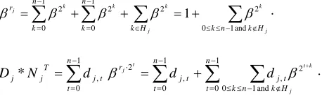
D=AB can be computed by the following formula [3], [4], [5]:
1 0 2 2 1 0 n i j n j i j i b a AB D v i j j i j n j j i n i i i j i i a b b a b a 1 2 ) 1 2 ( 1 0 1 0 2 ) 1 2 ( ) ( 0
. (1)
v
i k S
n j j j i j j i n i i i i k j i a b b a b a 1 1 0 2 1 0 2 1
. (2)
Recall that Ai is defined as Ai A i
2
, now we define B & An-i as follows:
B & An-i=
(
a
ib
0,
a
i1b
1,...,
a
i 1b
n 1)
. (3)Viewing B & An-i as a field element, we have n i k
n
j
j j
i b B A
a jk ( & )
1
0
2 and (2) may be
rewritten as follows:
D
v
i k S
k i n i n i B A A B A B 1
1 & &
& . (4)
Furthermore, we define R[i] as follows:
even. is if & odd, is if ) & ( ) & ( ] [ , 1 1 where ) & ( ) & ( ] [ n B A n B A A B v R v i B A A B i R v v n v n i n i n
Then we have
D=(B & A)1+
v
i k S
k i i R 1 ]) [
( . (5)
The RH algorithm for n odd is based on this formula, and it is presented in Appendix 1. For n
even, (5) may be further improved by Lemma 1 of [3]. Please refer to [4] and [5] for more details.
Since 0 k n 1, we may interchange the order of the summation in (5) and obtain the
formula:
k n
k i i v k Si
i R A B D 1
0 : 1 and
1 []
& . (6)
Based on this formula, an improved software multiplication algorithm, which is called A1, is
presented in Appendix 2.
Now we show the second improvement. From (3) we know that
(A & B)i=
i
B A& )2
( =
(
a
n ib
n i,
a
n i 1b
n i 1,...,
a
n 1b
n1,
a
0b
0,...,
a
n i 1b
n i1)
=(Ai & Bi).Thus (4) can be rewritten as:
v
i k S
i k k i k k i B A A B A B D 1 1
1& & & . (7)
Since elements of Si are in the range of [0, n-1], (7) can be rewritten as:
1
0 : 1 and 1
1& & &
n
k i i v k S
i k k i k k i B A A B A B D 1
0 : 1 and : 1 and 1
1& & &
n
k i i v k S
i k k S k v i i i k k i i B A A B A
B . (8)
Based on this formula, a software multiplication algorithm, which is called A2, is presented in
Appendix 3.
Similarly, for even n, we have the following formula:
1
1 1
1& & & &
v
i k S
v k k S k i k k i k k v i A B B A A B A B D . 1
0 :1 and : 1 1 and 1
1& & &
n
k i i v k S
i k k S k v i i i k k i i B A A B A
B . (9)
3. Proposed Algorithm And Software Implementations
From now on, we assume that the multiplicative order of the normal element is m, i.e., m is the
least positive integer such that m 1.
Definition 1. Ordered cyclotomic cosets mod m are the following ordered sets:
C0={<20>m, <21>m, <22>m,...,<2n-1>m}, <20>m=1 is called the coset leader;
Ci={<(2i+1)20>m, <(2i+1)21>m, <(2i+1)22>m,...,<(2i+1)2n-1>m}, where 0<i<n and
<(2i+1)20>m is called the coset leader.
In this definition, Ci is an ordered set and elements of Ci need not to be distinct. For example,
C1={3, 6, 12, 3, 6, 12} for m=21 and n=6. Sometimes we also view Ci as a set and call it the set
Ci. The following lemma shows that there are at most v+1 distinct sets Cis.
Lemma 1. For 0<i<n, the set Ci and the set Cn-i are identical.
Proof: It follows immediately from the fact m|(2n-1) and the congruence
i i n n i
i 1 2 2 (2 1)2
2 mod (2n-1).
To clarify the description of the new algorithm, we first give a simple example.
3.1 An Example
GF(28) has been standardized for space communication by ESA and NASA, and for use in CD
players [20], so it is desirable to design low complexity multipliers for the field. Gaussian NB is
widely used to design low complexity NB multipliers. But no GNB exists in GF(28). In Section 5,
we will show that the time complexity of the proposed GF(28) NB multiplier matches the best
result available in the open literature and its gate complexity is less than the best result.
Let GF(28) be a root of the irreducible polynomial f(x)=x8+x7+x6+x4+x2+x+1. From
Appendix C of [14], we know that is a normal element of multiplicative order 17.
Consider the following 3 OCCs mod 17:
C0 = {20, 21, 22,...,27} = {1, 2, 4, 8, 16, 15, 13, 9} with the coset leader r0=20=1;
C1 = {3.20, 3.21, 3.22,...,3.27} = {3, 6, 12, 7, 14, 11, 5, 10} with the coset leader r1=3.20=3;
C4 = {0, 0, 0, 0, 0, 0, 0, 0} with the coset leader r4=0.
For 0 i 4, <2i+1>17 belongs to just one OCC, i.e.,
i=0: <20+1>17=2 C0 and 2f e 2i 1
i
i r mod (17) holds for e
0=0 and f0=1;
i=1: <21+1>17=3 C1 and 2 e 2i 1 f
i
i r mod (17) holds for e
1=1 and f1=0;
i=2: <22+1>17=5 C1 and 2 e 2i 1 f
i
i r mod (17) holds for e
i=3: <23+1>17=9 C0 and 2f e 2i 1
i
i r mod (17) holds for e
3=0 and f3=7;
i=4: <24+1>17=0 C4 and 2 e 2i 1 f
i
i r mod (17) holds for e
4=4 and f4=0;
where the congruence 2 2i 1
e f
i
i r mod (17) means that <2i+1>
17 is the fi-th element of the
OCC
i
e
C
and fi is the smallest nonnegative integer such that the congruence holds.Associated with each Cj (j=0, 1, 4), a GF(28) vector Nj=(( rj)20,( rj)21,( rj)22,...,( rj)281) is
defined as follows:
N0=N=( , , ,..., )
1 8 2 1 0
2 2 2
2 ;
N1=( , , ,..., )
1 8 2 1
0 2 2 2
2 ; where 3 2 16 32 128
and
N4= (1,1 ,1 ,1 ,1 ,1 ,1 ,1 )
0
2
0 .
Let T
i
i a a a N
a
A i ( 0, 1,..., 7)
7
0
2 and T
i
i b b b N
b
B i ( 0, 1,..., 7)
7
0
2 be two elements
of GF(28). D=AB can be computed by the following formula:
D=AB=(a7b7, a0b0, a1b1 ,...,a6b6)*NT + (a0b1+b0a1, a1b2+b1a2 ,...,a7b0+b7a0)*N1T +
(a2b4+b2a4, a3b5+b3a5 ,...,a1b3+b1a3)*N1T + (a1b4+b1a4, a2b5+b2a5 ,...,a0b3+b0a3)*NT +
(a0b4, a1b5, a2b6,...,a7b3)*N4T
=T0*NT+T1*N1T+T2*N1T+T3*NT+T4*N4T.
The five inner products are denoted as T0*NT, T1*N1T, T2*N1T, T3*NT and T4*N4T, as shown
above. Arrays ei and fi (0 i 4) are used to determine these inner products, e.g.,
T e f f f f f
f f f T
N a
b b
a a b b a a
b b a N
T2* 1 ( 8 2 28 2 8 2 2 8 2),( 3 5 3 5),...,( 8 2 12 8 2 1 8 2 1 28 2 1)* 2 ,
where f2=6 and e2=1.
Now T0 and T3 have already been represented in the NB N. T1 and T2 can be combined into one
vector. After converting this vector and T4 into the GF(2) vector representation w.r.t. N, we get the
GF(2) vector representation of D=AB w.r.t. N.
3.2 Ordered Cyclotomic Cosets mod m
Lemma 1 shows that there are at most v+1 distinct sets Cis. However, the accurate number is
the number of different sets Cis. The following procedure determines the value of u and these sets.
INPUT: m (the order of the normal element).
OUTPUT: 1. integer u, OCC Cj's, where 0 j u 1;
2. arrays rj, ei and fi, where 0 j u 1 and 0 i v.
S1: set R = ;
S2: OCC C0 = {<20>m, <21>m, <22>m,...,<2n-1>m};
S3: r0=20=1; e0=0; f0=1; R = R C0; u=1;
S4: for i=1 to v do
S5: if <2i+1>m R then { /* a new OCC */
S6: OCC Cu = {<(2i+1)20>m, <(2i+1)21>m, <(2i+1)22>m,...,<(2i+1)2n-1>m};
S7: ru=<(2i+1)20>m; ei=u; fi=0; R = R Cu; u=u+1;
}else{
S8: Find j such that 0 j u 1 and <2i+1>m Cj ;
S9: Let f be the smallest nonnegative integer such that 2f.rj 2i+1 mod (m);
S10: ei=j; fi=f; }
Notes: 1. Since the proposed algorithm is applicable only to GF(2n) that the value of m is small,
one may first use reference [10] to find a small factor of 2n-1, and then check the existence of a
normal element whose multiplicative order equals this factor.
2. The following expression holds for 0 i v:
i i i
e m e f
m
i 1 2 r C
2 . (10)
Arrays ei and fi will be used in the proposed algorithm, and they have the following meaning:
<(2i+1)20>m is the fi-th element of the OCC
i
e
C
, where fi is the smallest nonnegative integer suchthat (10) holds.
Associated with each OCC Cj, a GF(2n) vector Nj is defined as follows, where 0 j u 1:
Nj=(( rj)20,( rj)21,( rj)22,...,( rj)2n1). (11)
Since r0=1, we have N0=N. It is easy to see that the vector Nj possesses the following property:
T j n n
T j
n N a a a a N
a a
a , ,..., ) ( , , ,..., )
( 1 0 1 2
2 1 1
3.3 New Multiplication Algorithm
We assume that n is odd, unless otherwise stated. Recall that the multiplicative order of is m.
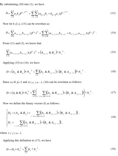
By substituting (10) into (1), we have
D v i r j j i j n j j i n j r j j j i f i e j f e a b b a b a 1 2 1 0 1 0 2 ) ( 0
0 . (13)
Now let k=fi+j, (13) can be rewritten as:
D v i r f k k f i f k n k k f i n k r f k f k k i e i i i i k e a b b a b a 1 2 1 0 1 0 2 ) )( ( ) ( 0 0 0
. (14)
From (11) and (3), we know that
T e f i f r f k n k k f
i i i i
k i e i
i b A B N
a )( ) & *
( 2
1
0
. (15)
Applying (15) to (14), we have
v i T e i f f i f f T e f
f B N Ai B i Bi A i Ni
A D 1 * & & & 0 0 0
. (16)
Since e0=0, f0=1 and 0 ei u 1, (16) can be rewritten as follows:
1
0 : and 1 0
1
1& & & *
u j T j v i e j i i f f i f f T N A B B A N B A D i i i i i
. (17)
Now we define the binary vectors Dj as follows:
v i e j i i f f i f f j v i e i i f f i f f f f i i i i i i i i i i A B B A D A B B A B A D 1 and : 1 and 0 : 0 , & & , & & ) & ( 0 0 (18)
where 1 j u 1.
Applying this definition to (17), we have
1 1 0 0 * u j T j j T N D N D
D . (19)
Since N0=N, D0 is just the GF(2) vector representation of D0*NT w.r.t. the NB N. Each Dj*NjT
(0<j<u) is also a field element, but Dj is not the GF(2) vector representation of Dj*NjT w.r.t. N. So
we need to convert Dj*NjT into the GF(2) vector representation w.r.t. N. This may be done by the
dj,0)2 be the binary representation of Dj and w (0<w<n) be the block size. We first divide Dj into
w
n blocks Dj,h as follows:
1 0 2 , 2 1 0 1 0 2 , 1 0 1 0 2 , 1 0 2 , *
wn wh
wh w n i w n i wh i h h j h w i i wh j h w i i wh j n i i j T j
j N d d d D
D , (20)
where rj and the binary representation of the block D
j,h is (dj,wh+w-1,...,dj,wh+1, dj,wh)2. In (20),
the term dj,i is defined as dj,i=0 for n i w wn 1.
The GF(2) vector representation of Dj*NjT w.r.t. N can be computed by the GF(2n) addition
operation if the GF(2) vector representation of each Dj,h w.r.t. N is available. In software
implementations, the GF(2) vector representation of Dj,h is stored in the precomputation table TB,
which is defined as follows:
for j=1 to u-1 do
for c=0 to 2w-1 do {
Let (cw-1cw-2 ... c1c0)2 be the binary representation of the integer c;
TB[j][c] = GF(2) vector representation of
1 0 2 w i r i i j
c w.r.t. N;}
Note that the table TB depends only on N, i.e., once the NB is chosen the table can be created
during the precomputation stage.
Since the binary representation of the block Dj,h is (dj,wh+w-1,...,dj,wh+1, dj,wh)2, (20) can be
rewritten as follows:
1 0 2 2 , 1 , 1 , ,..., , ) ] ][( [ * w n wh h wh j wh j w wh j T j
j N TB j d d d
D . (21)
Thus D=AB can be computed by the following formula.
1 1 1 0 2 2 , 1 , 1 ,
0 [ ][( ,..., , ) ]
u j h wh j wh j w wh j wn wh d d d j TB D AB
D . (22)
Based on (18), (19), (22) and Section 2.1, it is straightforward to present the following
multiplication algorithm for odd values of n.
Multiplication Algorithm A3 for n Odd:
OUTPUT: D=AB.
S1: Compute DAi and DBi for 0 i z;
S2:
0 0 &
0 Af Bf
D =(A&B)1 ;
S3: for j = 1 to u-1 do Dj=(0,0,...,0);
S4: for i = 1 to v do e e f f i f f i
i i i
i i
i D A B B A
D & & ;
S5: for j = 1 to u-1 do
S6: for h = 0 to wn -1 do D
0 = D0 (TB[j][Dj,h])wh;
S7: Output D0;
Notes: 1. Similar to Algorithm A1, starting addresses of f f i f f i
i i i
i A B B
A , , , and
i
e
D in S4
may be stored sequentially in a 1-dimensinal array for 1 i v. The size of this array is 5vz bits.
2. Since TB[j][Dj,h] is a GF(2n) element represented in the NB N, (TB[j][Dj,h])wh may also be
precomputed by the method introduced in Section 2.1. In S6, only wh-fold cyclic shifts of the
binary vector representation of TB[j][Dj,h] are required, thus it is easy to see that when w is
selected as a multiple of the minimal width of the data-path of the CPU, TB has the smallest size:
2n(u-1)2w bits. In our experiment, the value of w is 8.
Similarly, we have the following formula for even n:
T e v f f T
v v
v B N
A N B A
D 1 & 1 0 &
1
1
* &
& v
i
T e i f f i f
fi B i Bi A i N i
A . (23)
Recall that the multiplicative order of the normal element is m, and m is a primitive factor of
2n-1=(2v-1)(2v+1), i.e., m|2v+1, we know that ev=u-1, fv=0 and Nu-1=(1,1,...,1) in the output of the
procedure of Section 3.2. So (23) may be rewritten as
T u v T
N B A N B A
D 1& 1 0 0& 1
1
1
* &
& v
i
T e i f f i f
fi B i Bi A i Ni
A , (24)
where 0 ei u 2 for 1 i v 1
We may also compute the product D=AB using a lookup table. Since Nu-1={1,1,...,1},
(A0&Bv)*Nu-1T is actually an element of GF(2), which is equal to the parity of (A0&Bv). This
3.4 Analysis and Comparison of Software Implementations
The time complexity of the RH algorithm is determined in [4] and [5]. It needs n n-bit AND
operations and
2 1 2
1 CN
n =(C n 2)/2
N n-bit XOR operations. The number of n-bit cyclic shift
operations of the RH algorithm is equal to (CN+2n-1)/2.
Ning and Yin presented two algorithms in [13]: one is for ONB and the other is for nonoptimal
normal bases. The algorithm for nonoptimal normal bases is slow, and we only consider the one
for ONB. Since no description of the precomputation procedure was presented in [13] (parts of the
NY algorithm were described in a patent application), we assume that the method introduced in
Section 2.1 is used to perform this precomputation. For the NY algorithm, DAj and DBj are
defined as z n
z -bit vectors, thus the total number of cyclic shift operations is about 2z. Based on
this assumption, we know that the NY algorithm 3 of [13] requires about 2n n-bit XOR, n+1 n-bit
AND and 2z n-bit cyclic shift operations.
Now we analyze the space complexity of Algorithm A3.
In line S1, 4zn bits are required to store arrays DAj and DBj (0 j z). In line S2 and S3,
variables Djs (0 j u 1) require un bits. Note 2 shows that the table TB[j][Dj,h] requires
2n(u-1)2w bits. Therefore the space complexity of Algorithm A3 is 4zn+un+2n(u-1)2w bits.
This size is reasonable on modern 32-bit computers. For example, if w=8 then it is 2709966 bits
( 331 Kbytes) for GF(2571) (u=10).
In Algorithm A3, starting addresses of , , , , ,
i i i i
i f i f f i e
f B B B D
A and (TB[j][Dj,h])wh may be
computed in the precomputation procedure, so it is easy to determine the time complexity.
The cyclic shift operation is required only in line S1. From Section 2.1, we know that the total
number of cyclic shift operations in the algorithm is 4z.
The numbers of AND operations in line S2 and S4 are 1 and 2v=n-1, respectively. Thus the
algorithm requires n AND operations.
For simplicity, we suppose that the statement Dj=(0,0,...,0) of S3 can be performed at the cost of
line S6 is repeated (u-1) w
n times. Therefore the total number of XOR operations used in the
algorithm is ( w
n +1)(u-1)+n-1.
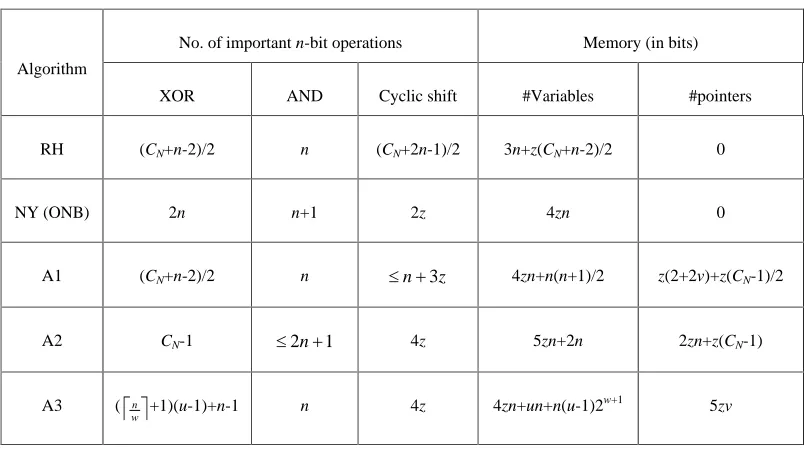
Table 1 compares the time and space complexities of these NB algorithms in GF(2n) where n is
odd. In the table, #Variables denotes the size of the temporary variables, and #Pointers denotes the
size of the 1-dimensional array discussed in Note 1 of Algorithms A1, A2 and A3.
TABLE 1: Comparison of NB multiplication algorithms (n odd).
No. of important n-bit operations Memory (in bits) Algorithm
XOR AND Cyclic shift #Variables #pointers
RH (CN+n-2)/2 n (CN+2n-1)/2 3n+z(CN+n-2)/2 0
NY (ONB) 2n n+1 2z 4zn 0
A1 (CN+n-2)/2 n n 3z 4zn+n(n+1)/2 z(2+2v)+z(CN-1)/2
A2 CN-1 2n 1 4z 5zn+2n 2zn+z(CN-1)
A3 (
w
n +1)(u-1)+n-1 n 4z 4zn+un+n(u-1)2w+1 5zv
We assume that the general-purpose processor can perform 1 n-bit XOR or AND operation
using 1 n-bit operation. As defined in [5], we also assume that 1 cyclic shift operation needs
n-bit operations. Our experiments and [5] show that the value of is typically 4 for the C
programming language if only simple logical instructions, such as AND, SHIFT and OR are used
to emulated a k-fold cyclic shifts. Now we compare these algorithms. We assume that w=8, =4
and z=32, and obtain the following results:
1. Algorithm A1 is faster than the RH algorithm if CN > 193.
2. Algorithm A1 is faster than Algorithm A2 if CN > 7n - 258.
3. Algorithm A3 is faster than the NY algorithm if n > 292 and
even. 3
odd, 2
n n
u .
2 2
256 7 1
8
n N n
C
u . (25)
Appendix 4 contains 204 values of n such that 100<n<1001 and the inequality (25) is satisfied.
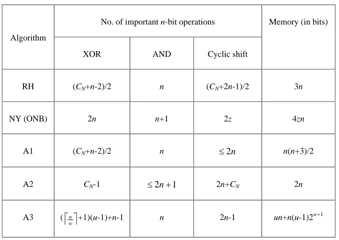
For memory constrained systems, Hasan proposed a lookup table-based polynomial basis
multiplication algorithm in [9]. The size of the tables is (w+d)2w, where d is the degree of the
second leading coefficient of the field-defining polynomial. Now we consider these NB
algorithms in such systems. For Algorithms A1, A2 and A3, we will not use arrays DA, DB and the
1-dimensional array introduced in Note 1 of these algorithms. Furthermore, we assume that values
of ek and cyclic shift count are hard-coded [5], i.e., they are stored as program codes. Table 2
compares the time and memory complexities of these NB algorithms. From the table, we conclude
that RH and NY algorithms are better choices in memory constrained systems.
TABLE 2: Comparison of NB algorithms in memory constrained systems (n odd).
No. of important n-bit operations Algorithm
XOR AND Cyclic shift
Memory (in bits)
RH (CN+n-2)/2 n (CN+2n-1)/2 3n
NY (ONB) 2n n+1 2z 4zn
A1 (CN+n-2)/2 n 2n n(n+3)/2
A2 CN-1 2n 1 2n+CN 2n
A3 (
w
n +1)(u-1)+n-1 n 2n-1 un+n(u-1)2w+1
We implement these NB multiplication algorithms in ANSI C using Microsoft Visual C++ 6.0
complier. For comparison, we also implement the polynomial basis multiplication algorithm
presented in [6], i.e., the finite field analogue of the Montgomery multiplication for integers. For
simplicity, the Montgomery multiplication algorithm is implemented in GF(2k) instead of GF(2n),
where w n
w
modern 32-bit computers. So we also select w=8, and employ the table lookup approach, which is
shown to be the best choice to perform word-level multiplications [6].
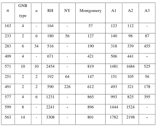
Our experiments are performed on an IBM ThinkPad 770X notebook with a 300 MHz Pentium
II CPU running Windows NT 4.0. Experimental results are listed in Table 3, where the first five
fields are the binary fields recommended by NIST for ECDSA applications. Since the NY
algorithm is slow for nonoptimal normal bases, we do not list timings for these fields. For GF(2n)
that the value of u is large, the timing of A3 do not listed in the table either. In Table 3, Algorithm
A2 is slightly slower than the Montgomery algorithm for GF(2409). So for applications that many
squaring operations are required, e.g. exponentiation, Algorithm A2 is a better choice.
TABLE 3: Timings for some GF(2n)s ( s)
n
GNB type
u RH NY Montgomery A1 A2 A3
163 4 - 164 - 57 123 112 -
233 2 6 180 56 127 140 98 87
283 6 34 516 - 190 318 339 455
409 4 - 671 - 421 506 441 -
571 10 10 2454 - 819 1481 1684 525
251 2 2 192 64 147 151 105 56
491 2 2 590 226 612 493 321 178
577 4 6 1231 - 865 993 825 395
599 8 - 2241 - 896 1444 1524 -
563 14 - 3308 - 801 1782 2198 -
4. Mathematical Properties
We now present some mathematical properties of the new algorithm.
Recall the definition of the primitive factor of 2n-1 in [15, p.173].
Lemma 2. If p is a primitive factor of 2n-1, then <p>n=1. If n odd, <p>8= 1; if <n>8= 2, <p>8=1
or 3; if <n>8=0, <p>2n=1 [15].
Given two GF(2n) normal elements A and B of multiplicative orders a and b, respectively. If a|b
then the number of different sets Cis mod a is not greater than that of b. Thus selecting A results in
a better implementation of the algorithm. From [25 Theorem V], we know that 2n-1 (n>1) posses
at least one primitive factor with the single exception n=6. So we only consider the normal
element of the prime order in this paper. We define the type of a normal element as follows:
Definition 3. A normal element of GF(2n) over GF(2) is said to be of type k if its multiplicative
order is kn+1 and kn+1 is a primitive factor of 2n-1.
It seems that the smaller multiplicative order may result in the smaller value of u, which in turn
results in a faster implementation of the proposed algorithm. But this is not always true. For
example, 328177=318*1032+1 and 359137=348*1032+1 are two primitive factors of 21032-1, and
in GF(21032) we have found two normal elements of orders 328177 and 359137, respectively. Our
experiments show that their values of u are 268 and 267, respectively.
Now we show the relation between the GNB and the type k normal element. The type-I GNB
are always called the type-I ONB, and they are determined by the following lemma [7]:
Lemma 3. GF(2n) contains a type-I ONB iff n+1 is a prime and 2 is a primitive root mod n+1.
From this lemma, the following theorem holds immediately.
Proposition 1. GF(2n) contains a type 1 normal element iff n+1 is a prime and 2 is a primitive
root mod n+1.
All type-II GNB, which are called type-II ONB, are described by the following lemma [7,8]:
Lemma 4. If
(1) 2 is primitive in Z2n+1, or
(2) 2n+1 is a prime congruent to 3 modulo 4 and 2 generates the quadratic residues in Z2n+1,
Let be a primitive (2n+1)st root of unity in GF(22n) and 1. Then is a type-II
ONB generator.
If condition (1) holds then (2n+1) 2n-1, and there is no element of order 2n+1 in GF(2n). We
(2n+1) is a primitive factor of 2n-1. We may expect that either or -1, but not both, is a normal
element of type 2. But this is not true. Our experiments show that for n<2000 such that the second
class of type-II ONB exists in GF(2n), there are three fields that do not contain type 2 normal
elements: GF(2119), GF(2791) and GF(21659).
On the other hand, there exist type 2 normal elements in some GF(2n)s but no type-II ONB
exists in these fields. For example, Appendix 4 lists some values of n such that 8|n and type 2
normal elements exist in GF(2n). But there is no GNB exists in these fields.
We now present some additional differences between the type t GNB and type t normal
elements:
1. For some values of n and t (t>2) there exists type t GNB in GF(2n) but no normal element
with u=t exists in the field, and vice versa.
2. For a given GF(2n) and the value of t, the field can have, at most, one type t GNB, but the
field may contain more than one type t normal elements up to conjugacy, e.g., GF(2468)
have 6 type 16 normal elements up to conjugacy.
3. GNB generators always have high multiplicative orders, and are very often primitive [19].
5. New Bit-Parallel Multiplier
5.1 Architecture
We now assume that n is odd, unless otherwise stated. Because we have described the proposed
algorithm for software implementations in detail, it is easy to understand its application to VLSI
multipliers. The new multiplier works in a similar way of software implementations: it first
computes each Dj=(dj,0,dj,1,...,dj,n-1) by (18) and then converts each dj,k into the coordinate w.r.t. the
selected NB N.
The new multiplier first computes aibj (0 i,j n 1), which is called a term, using exactly n2
two-input AND gates. This operation requires a single AND gate delay TA due to the parallelism.
Then it computes coordinates of Dj=(dj,0,dj,1,...,dj,n-1) by (18) as follows:
v i e j i
i f k f k i f k f k k
j
v i e i
i f k f k i f k f k f
k f k k
i
i i i
i i
i i i
i
a b b
a d
a b b
a b
a d
1 and : ,
1 and 0 : ,
0
,
,
0 0
where 0 k n 1 and 1 j u 1.
For a fixed j and 0 k n 1, each dj,k has the same number of terms, which is denoted as |dj,k|.
Since each term aibj (0 i,j n 1) is XORed only once, the total number of two-input XOR gates
required in this step is n2-nu.
For 0 j u 1, dj,0 may be computed using a binary XOR tree, and the time delay is at most
|) (|
log2Max dj,0 TX due to the parallelism, where TX is the delay of one two-input XOR gate.
Since d0,k is already the coordinate representation w.r.t. N, we now need to convert each dj,k
(1 j u 1) into the coordinate representation w.r.t. N.
For 1 j u 1, let 1
0 2 , n t t j r t
j be the expansion of j
r
w.r.t. N, where j,t GF(2) and
(10) holds for some i such that 1 i v and ei=j. Let Hj t| j,t 1 and hj=|Hj|. We may rewrite
Hj as { ,1, ,2,..., , }
j
h j j j
j w w w
H , where0 w,1 w,2 ... w, n 1
j
h j j
j , and obtain the following
identity: j k j w j k j h k H k r 1 2 2 ,
. (27)
By (11), we know that
j k j w t j k j w t t j h k n t t j n t h k t j n t r t j T j
j N d d d
D 1 2 1 0 , 1 0 1 2 , 1 0 2 , , ,
* . (28)
The coefficient of in (28) is
j k j h k w n j d 1 , ,
. Therefore, from (19) we know that the expression
of d0, which is the coefficient of in the final result of D=AB=(d0,d1,...,dn-1), is
1 1 1 , 0 , 0 0 , u j h k w n j j k j d d
d . (29)
The term d0 may be computed by a binary XOR tree, which requires
1
1
u
j j
h XOR gates and
1 1 2 1 log u j j
h TX gate delay. Therefore the total number of XOR gates required in this
conversion step is n 1
1
u
j j
values of j, the delay of 1 1 2 1 log u j j
h TX in this conversion step is an upper bound. Take
GF(2468) (u=17) for example. For 0 j u 1, values of |dj,0| are 29, 30, 34, 30, 32, 32, 22, 24, 24,
22, 26, 36, 36, 26, 36, 28 and 1, respectively. There are 6 type 16 normal elements up to
conjugacy, and values of 2
1
u
j j
h for these normal elements are 3424, 3444, 3420, 3448, 3468, and
3456, respectively. We select the normal element of 2
1
u
j j
h =3420 to represent field elements. For
this normal element, values of hj are 232, 253, 233, 236, 225, 241, 216, 228, 229, 221, 225, 228,
216, 228 and 209, respectively, where 1 j u 2.
From values of |dj,0|, it is easy to see that generating d0,k, d1,k, d3,k, d4,k, d5,k, d6,k, d7,k, d8,k, d9,k,
d10,k, d13,k and d15,k requires 5TX and generating d2,k, d11,k, d12,k and d14,k requires 6TX, where
1
0 k n . In (29), terms generated in 5TX may be first XORed pairwisely, and then these
summations and terms generated in 6TX are XORed. The accurate time delay of this computation
procedure is log 934 2486/2
2 TX=12TX, where 934=h2+h11+h12+h14=253+225+228+228 and
2486= 2 1 u j j h -934=3420-934.
For even values of n, we have the following formula from (24):
, , , , 1 1 1 and : , 1 1 and 0 : ,
0 0 0
v k k k u v i e j i i f k f k i f k f k k j v i e i i f k f k i f k f k f k f k k b a d a b b a d a b b a b a d i i i i i i i i i i (30)
where 0 k n 1 and 1 j u 2.
The conversion step for n even is similar to that of n odd. The only difference is g = Du-1*Nu-1T.
From the discussion after (24), we know that Nu-1=(1,1,...,1) and g GF(2). Therefore we may
first compute g using n-1 XOR gates and then XOR this single bit to each dk (0 k n 1) at the
cost of n XOR gates. This method needs only 2n-1 XOR gates.
In [22], this idea was generalized. Converting Dj*NjT (1 j u 1) into the coordinate
the following variants of (27) and (28): j k j k k k j H k n k H k n k n k r and 1 0 2 2 1 0 2 1 0
2 1 . (31)
1
0
1
0 0 1and 2 , , 1 0 2 , * n t n
t k n k H
t j t j n t r t j T j j j k t t j d d d N
D . (32)
Formula (32) requires n+n(n-hj) XOR gates to convert Dj*NjT.
5.2 Analysis and Comparison of Bit-Parallel Multipliers
The gate and time complexities of the new multiplier are listed in Table 4, where complexities
of the multiplier in [3] are also listed. In the table, Max(|dj,0|) denotes the maximum value of |dj,0|
for 0 j u 1.
TABLE 4: Comparison of two NB multipliers.
Multipliers #AND #XOR Time Delay
Proposed
(n odd)
n2 n2-nu+n
1
1
u
j j
h TA+ log2Max(|dj,0|) TX+ 1
1 2 1 log u j j
h TX
Proposed
(n even)
n2 n2-nu+2n-1+n
2
1
u
j j
h TA+ log2Max(|dj,0|) TX+
2 1 2 2 log u j j
h TX
[3] Theorem 2 n2 n(CN+n-2)/2 TA+ log2(CN 1) TX
Since it is not easy to determine the explicit expression of hj, we assume that hj=n/2 and CN=tn
for simplicity. Based on this assumption, we know that numbers of XOR gates required by two
multipliers are about u n2 nu
2 ) 1
( and
n n t 2 2 ) 1
( , respectively. Therefore the new algorithm
may be used to design multipliers in GF(2n)s such that u<t. As enumerated in Appendix 4
(100<n<1001), there are 25 n values such that 8 n and u<t.
Now we analyze the time complexity of the new multiplier. In Table 4, Max(|dj,0|) is used to
determine the time delay. For a fixed j and 0 k n 1, each dj,k has the same number of terms,
and |dj,k|=n/u on average. Thus, time complexities of two multipliers are about TA+ log ( 2/2)
2 n TX
multiplier is larger than [3]. For a randomly selected NB, the average value of t is n/2 and the time
delay of two multipliers are equal. So for GF(2n) that no GNB exists (8|n) and the value of u is
small, the algorithm provides an new way to design multipliers in these fields. In Appendix 4
there are 22 n values such that u<12 and 8|n.
We now show the performance of the new multiplier with four examples.
In [1] and [3], two type-I ONB multipliers are presented. Both multipliers require n2-1 XOR
gates and n2 AND gates. Their gate delays are
X
A n T
T 2 log2( 1) and TA 1 log2(n 1) TX,
respectively. For GF(2n) where type-I ONB exists, N0=N and N1=(1,1,...,1). Since d1,0 consists of a
single term, no XOR gate is required to compute D1. It is easy to see that n(n-2) XOR gates are
required to compute D0. Computing g=D1*N1T, which is the parity of D1, requires n-1 XOR gates,
and the gate delay is log2n TX. The final result is obtained by adding this bit to every bits of D0,
and this needs n XOR gates and 1TX gate delay. Thus the total number of XOR gates is n2-1 and
the gate delay is
X
A n T
T 1 log2 . Since log2n log2(n 1) for n>3 and 8 n, the new
multiplier matches the best result presented in Table 3 of [3].
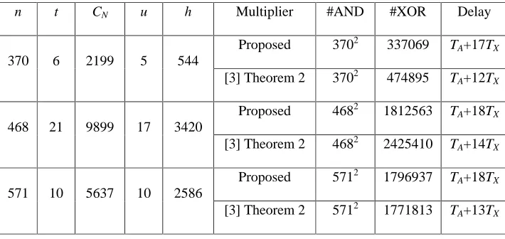
Table 5 shows a comparison of the new multiplier with the multiplier of [3] in three fields:
GF(2370), GF(2468) and GF(2571). From [24], we know that there exist cryptographically
interesting elliptic curves in GF(2468). Since the signal reuse method introduced in [3] is
applicable to both multipliers, it is not used here. In Table 5, t denotes the GNB type and h
denotes the minimal value of 1
1
u
j j
h (n odd) or
2
1
u
j j
h (n even).
TABLE 5: Comparison of NB multipliers for GF(2370), GF(2468) and GF(2571)
n t CN u h Multiplier #AND #XOR Delay
Proposed 3702 337069 TA+17TX
370 6 2199 5 544
[3] Theorem 2 3702 474895 TA+12TX
Proposed 4682 1812563 TA+18TX
468 21 9899 17 3420
[3] Theorem 2 4682 2425410 TA+14TX
Proposed 5712 1796937 TA+18TX
571 10 5637 10 2586
5.3 An Example
Now we illustrate the proposed multiplier for GF(28). From Section 2.1, we have the following
formulas for D0, D1 and D2:
D0=(d0,0, d0,1,...,d0,7)=T0+T3=(x1,4+a7b7, x2,5+a0b0 ,...,x0,3+a6b6),
D1=(d1,0, d1,1,...,d1,7)=T1+T2=(x2,4+x0,1, x3,5+x1,2 ,...,x1,3+x7,0) and
D2=(d2,0, d2,1,...,d2,7)=T4=(a0b4, a1b5, a2b6,...,a7b3), where xi,j=aibj+ ajbi.
Computing D0 and D1 requires 2n+3n=40 XOR gates, and no XOR gate is required to compute
D2. Recall that N2={1,1,...,1}, the value of g=D2*N2T is equal to the parity of D2, which can be
computed using n-1=7 XOR gates. Since N1={ , ,..., }
1 8 1
0 2 2
2 , where 21 24 25 27
,
we have the following formulas for D=AB=(d0, d1,...,d7):
d0=d0,0+g+d1,7+d1,4+d1,3+d1,1=d0,0+g+(d1,3+d1,7)+d1,1+d1,4,
d1=d0,1+g+d1,0+d1,5+d1,4+d1,2=d0,1+g+(d1,0+d1,2)+d1,4+d1,5,
d2=d0,2+g+d1,1+d1,6+d1,5+d1,3=d0,2+g+(d1,3+d1,6)+(d1,1+d1,5),
d3=d0,3+g+d1,2+d1,7+d1,6+d1,4=d0,3+g+(d1,2+d1,7)+(d1,4+d1,6),
d4=d0,4+g+d1,3+d1,0+d1,7+d1,5=d0,4+g+(d1,3+d1,7)+d1,0+d1,5,
d5=d0,5+g+d1,4+d1,1+d1,0+d1,6=d0,5+g+(d1,4+d1,6)+d1,0+d1,1,
d6=d0,6+g+d1,5+d1,2+d1,1+d1,7=d0,6+g+(d1,1+d1,5)+(d1,2+d1,7) and
d7=d0,7+g+d1,6+d1,3+d1,2+d1,0=d0,7+g+(d1,0+d1,2)+(d1,3+d1,6).
The signal reuse technique of [3] is employed in these formulas. Partial sums in the brackets
can be reused, e.g., both d0 and d4 have common terms (d1,3+d1,7). Therefore the total number of
XOR gates used in this conversion step is reduced from 40 to 34, and the total number of XOR
gates of the multiplier is 40+7+34=81.
Generating g needs 1 TA and 3 TX time delay, and generating each di,j needs 1 TA and 2 TX due to
the parallelism. So the total gate delay of the multiplier is 1TA+5TX.
From Table 2 of [21], we know that the minimal value of CN is 21 for GF(28), and the formula
for D=AB=(d0, d1,...,d7) is
xi+3, i+6 + xi+6, i+1 + xi+0, i+3 + xi+2, i+6 + xi+3, i+7 , where 0 i 7 and xk,j=a<k>b<j>+a<j>b<k>.
Using the symmetry property and the signal reuse technique of [3], we know that the GF(28)
multiplier of [3] requires 96 XOR gates and the total gate delay is 1TA+5TX.
6. Conclusions
We have proposed a new NB multiplication algorithm for GF(2n). The proposed algorithm
provides a new way to perform NB multiplication in some GF(2n)s. The complexity of the
proposed algorithm does not depend on CN but the multiplicative order of the normal element. For
these GF(2n)s, the new algorithm can be used to design not only fast software multiplication
algorithms but also low complexity bit-parallel VLSI multipliers. Especially, for some values of n
that no Gaussian NB exists in GF(2n), i.e., 8|n, the algorithm can still be used to design low
complexity VLSI multipliers.
The proposed algorithm speedups software implementations by look-up table. But for VLSI
implementations, the time complexity of the new multiplier is higher than the multiplier of [3] in
GF(2n) where low complexity NB exists.
Two improvements on RH algorithm have been shown. Both theoretical and experimental
comparisons of these NB algorithms have been presented. It is shown that they have specific
Appendix 1:
RH Multiplication Algorithm for n odd:
INPUT: A, B, Si, where 1 i v.
OUTPUT: D=AB.
S1: D = (A & B)1;
S2: for i = 1 to v do {
S3: R = (B & An-i) (A & Bn-i);
S4: for each k Si do D = D Rk; }
Appendix 2:
Multiplication Algorithm A1 for n Odd:
For each 0 k n 1, the following precomputation procedure is to find all values of i such that
v i
1 and
i
S
k .
A2.1 Precomputation:
INPUT: n, Si, where 1 i v.
OUTPUT: ek and m[k][j], where 0 k n 1and 0 j ek 1.
S1: for k = 0 to n-1 do ek =0;
S2: for i = 1 to v do {
S3: for each k Si do {
S4: m[k][ek] = i ;
S5: ek = ek+1; } }
This procedure outputs ek and m[k][j], where 0 k n 1 and 0 j ek 1. ek is the total
number of is such that 1 i v and k Si, and m[k][0] to m[k][ek-1] store these is, i.e., k Sm[k][j]
for 0 j ek 1.
A2.2 Algorithm A1 for n Odd:
INPUT: A, B, ek and m[k][j], where 0 k n 1and 0 j ek 1.
OUTPUT: D=AB.
S1: Compute DAi and DBi for 0 i z;
S2: D = A1 & B1= (A & B)1;
S3: for i = 1 to v do R[i] = (B & An-i) (A & Bn-i);
S4: for k = 0 to n-1 do
S5: if ek > 0 then{
S6: C = R[m[k][0]];
S7: for j = 1 to ek-1 do C =C R[m[k][j]];
S8: D = D (C >> k); } // C>>k denotes k-fold right cyclic shifts of C.
Notes 1: For each 1 i v, An-i is stored in n z successive computer words starting from
DA[s][t] and ending at DA[s][t+ zn -1], where t = i /z , s = i & (z-1) and & denotes the bit-wise
AND. In our implementation, these address computations are performed in the precomputation
procedure, and starting addresses of A1, B1, An-i, Bn-i and R[m[k][j]] are stored sequentially in a
1-dimensional array, where 1 i v, 0 k n 1 and 0 j ek 1. Since ( 1)/2
1 1
0
N v
i i n
k
k h C
e ,
the size of this 1-dimensinal array is z(2+2v) + z(CN-1)/2 bits.
2: Algorithm A1 may be implemented without computing arrays DA and DB. Experimental
results show that arrays DA and DB speedup Algorithm A1 by no more than 10% for GF(2n)s
listed in Table 3 of Section 3. For example, Algorithm A1 without computing arrays DA and DB
performs one multiplication operation in 1566 s over GF(2571).
A2.3 Complexity Analysis:
First we show that there is no need to define array DAj as a 2n-bit vector in line S1. Since only
i-fold left cyclic shifts of A is required in line S3, where 1 i v, we may define array DAj as a
(n+v)-bit vector.
DA0 = (a0,a1,...,an-1,a0,a1,...,av-1) and
DAj = (aj,...,an-1,a0,a1,...,av-1a0,...,aj-1), where 1 j z.
From this definition, we know that the time complexity to compute DAj's and DBj's (0 j z)
is about 3z n-bit cyclic shift operations, and 3zn bits are required to store these arrays.
The cyclic shift operation is also required in line S8. Since ek may be zero for some values of k,
one can see that the total number of cyclic shift operations in Algorithm A1 is at most n+3z. For
example, our experiments show that for 100<n<1000, where n is odd and the type-II ONB exists
in GF(2n), the minimal, average and maximal percentages that ek=0 are 22.9%, 25.0% and 27.2%
respectively.
XOR operations are required in S3, S7 and S8. In S3, the XOR operation is repeated v=(n-1)/2
times. Since 1 ( 1)/2
0
N n
k
k C
e , the total number of XOR operations in line S7 and S8 is (CN 1)/2.
Therefore the total number of XOR operations in Algorithm A1 is
2 1 2
1 CN
n =
2 / ) 2
In line S2 and S3, 1 and 2v=n-1 AND operations are required, respectively. Therefore
Algorithm A1 requires n AND operations.
Now we analyze the space complexity of Algorithm A1.
In line S1, arrays DAj and DBj (0 j z) need 3zn bits. In line S3, the array R[i] (1 i v)
requires vn bits. In line S5, the array ek (0 k n 1) requires zn bits. The temporary variable C
of S6 needs n bits. From Note 1, we know that there is no need to store the array m[k][j] in
Algorithm A1. Therefore the space complexity of the Algorithm A1 is 3zn+vn+zn+n =
Appendix 3:
Multiplication Algorithm A2 for n Odd:
We only present the algorithm for n odd. In this case, both Algorithm A1 and A2 share the same
precomputation procedure, which have been presented in Appendix A2.1.
A3.1 Algorithm A2 for n Odd:
INPUT: A, B, ek and m[k][j], where 0 k n 1and 0 j ek 1.
OUTPUT: D=AB.
S1: Compute DAi and DBi for 0 i z;
S2: D = A1 & B1= (A & B)1;
S3: for k = 0 to n-1 do
S4: if ek > 0 then{
S5: UA = A<k-m[k][0]>; UB = B<k-m[k][0]>;
S6: for j = 1 to ek-1 do { UA = UA A<k-m[k][j]>; UB = UB B<k-m[k][j]>; }
S7: D = D (Bk & UA) (Ak & UB); }
S8: Output D ;
Note 1: In our implementation, starting addresses of Ak, Bk A<k-m[k][j]>, and B<k-m[k][j]> in Algorithm
A2 are also computed in the precomputation procedure and stored in a 1-dimensional array, where
1
0 k n and 0 j ek 1. Since ( 1)/2
1
0
N n
k
k C
e , the size of this array is 2zn+z(CN-1) bits.
A3.2 Complexity Analysis:
Since DAj and DBj are defined as 2n-bit vectors, the number of cyclic shift operations, which
are required only in line S1, is 4z.
AND operations are required in S2 and S7. In line S2, one AND operation is required. Since ek
may be zero for some values of k, one can see that at most 2n AND operations are required in S7.
Therefore the total number of AND operations in Algorithm A2 is at most 2n+1.
Since 1 ( 1)/2
0
N n
k
k C
e , the total number of XOR operations in Algorithm A2 is CN-1.
Since DAj and DBj (0 j z) are defined as 2n-bit vectors in line S1, 4zn bits are required to
store them. In line S4, the array ek (0 k n 1) requires zn bits. Temporary variables UA and
UB of S5 need 2n bits. From Note 1, we know that there is no need to store the array m[k][j] in