ABSTRACT
FERRIER, PEYTON MICHAEL. Three Essays on Quality Differentiation. (Under the direction of Russell L. Lamb and Walter N. Thurman)
This dissertation includes three essays that consider the role of quality variation within agricultural production when consumers are heterogeneous in their preferences for quality. The first essay, “The Welfare Benefits of USDA Beef Quality Certification Programs,” estimates the consumer welfare benefits from the increase in scope of USDA beef quality certification programs in the 1990’s. Between 1975 and 1999, beef demand fell by 66% (Marsh, 2003) and its share of the overall meat market fell from 48% to 32%. Along with changing consumer preferences and heightened health consciousness, poor quality assurance has been offered as a reason for the decline. Certification programs provide producers a new way to differentiate and brand products as being of higher quality outside the USDA grading program. Between 1994 and 2002, the share of all commercial cattle that are certified rose from 4% to 12% and the share that are both certified and qualify as upper Choice rose from 3% to 8%. An Inverse Generalized Almost Ideal Demand System (IGAIDS) is estimated using weekly data on beef consumption by grade, branded beef, chicken and pork. It is found that the increase in branded beef supplies in 1990’s increased consumer welfare by approximately 2% of beef expenditure.
and losses of producers over the long run. Comparative statics and simulations also demonstrate that the size and distribution of total welfare are affected by the number of grades and the placement of grade standards. An overview of the USDA beef quality grading and certification programs is provided and related to the model.
The third essay, “When is Fruit Bundling Fruitless? Sorting, Bundling and Disposal When Quality Information is Asymmetric,” considers the conditions in which sellers allow sorting and discourage it through mechanisms such as bundling.
DEDICATION
To my father, William James Ferrier,
whose passion for the social sciences and mathematics
PERSONAL BIOGRAPHY
Peyton Michael Ferrier was born at Resurrection Hospital in Chicago, Illinois on October
27th 1975 as the youngest of four children to William and Dolores Ferrier. After
graduating from Archbishop John Carroll High School in Radnor, Pennsylvania in 1993,
he attended John Hopkins University in Baltimore, Maryland. After graduating with a
Bachelor of Arts degree in Economics with a minor in Math Sciences in 1997, he served
in the Americorps VISTA program at the Mountain Microenterprise Fund in Asheville,
North Carolina for one year. In 1998, he entered the doctoral program in economics at
North Carolina State University. In 2001, he married Kathryn M. Stahl at Grace
Methodist Church in Aberdeen, Maryland. In 2003, he accepted the position of Visiting
Instructor of Economics at Ursinus College in Collegeville, Pennsylvania
ACKNOWLEDGEMENTS
The author acknowledges his indebtedness to several people.
To Dr. Russell L. Lamb, for his patience, dedication and encouragement though the
writing this dissertation. From the earliest stages of this work, his direction and feedback
were critical to its successful completion.
To Dr. Walter N. Thurman, his keen insights into econometric modeling and sunny
optimism were invaluable.
To Dr. Charles R. Knoeber and Nicholas E. Piggott, who served as committee
members and provided crucial insights with the development of theoretical and statistical
models in this work.
To faculty members and graduate students of the North Carolina State University
Economics Department including Tom Vukina, David Flath, Steven Margolis, Kerry
Smith, Barry Goodwin, Duncan Holthausen, Alison Davis, Christopher Hopkins, Varun
Kshirsagar, Nick Kuminoff, Luiz Maia, Todd McFall, Bailey Norwood, and Matthew
Roberts. In ways too numerous to catalogue, these individuals continued the traditions of
collegiality, intellectual curiosity and critical analysis that underpin academic learning and
scientific advancement.
To Kathy Stahl, who assisted in the revision of this dissertation at critical
TABLE OF CONTENTS
List of Tables………vii
List of Figures………..viii
Chapter 1 – Introduction……….…1
Chapter 2 – The Welfare Benefits of USDA Beef Quality Certification Programs…5 I. Introduction……….6
II. An Overview of the Beef Industry………7
III. Research Questions on Welfare and Demand……….11
VI. Literature Review on Demand Estimation and Welfare Analysis………... 14
V. Description of the IGAIDS Model………...24
VI. Description of the Data………..……. 29
VII. Estimation Results………... 30
VII.A. Vertical Differentiation……….. 31
VII.B. Potential Future Consumer Welfare Gains………...…… 32
VIII. Conclusion……….………. 34
IX. Bibliography………36
X. Tables and Figures…...……….40
Chapter 3 – Grading and Quality Certification in Beef Production………. 55
I. Introduction……….56
II. An Overview of Beef Quality Evaluation………....57
III. Moral Hazard in Quality Production………. 63
IV. An Equilibrium Model of Grading……….. 65
IV.A. Producers and Supply……….…... 66
IV.B. Consumers and Demand……….... 71
IV.C. Supply and Demand in Equilibrium………... 75
IV.D. The Effect of Changing a Grading Standard………. 76
IV.E. The Effect of Introducing a New Grade………. 80
V. Simulation Results……….……….…. 83
VI. Summary and Conclusions……….. 87
VII. Bibliography………... 89
VIII. Tables and Figures………... 94
IX. Appendix………. 113
Chapter 4 – When is Fruit Bundling Fruitless? ………114
I. Introduction………..……….. 115
II. Literature Review………..………. 116
III. The Vertical Differentiation Model of Demand………... 121
III.B. Quality Discrimination……….………. 123
III.C. Market Clearing Under Asymmetric Information with Sorting…… 126
III.D. Comparing the Sorting and Bundling Equilibriums……….. 128
IV. Disposal as Quality Improvement……….. 132
V. Conclusion……….. 138
VI. Bibliography………... 140
VII. Appendix………. 141
VIII. Tables and Figures……….. 144
Chapter 5 – Conclusion………. 148
LIST OF TABLES
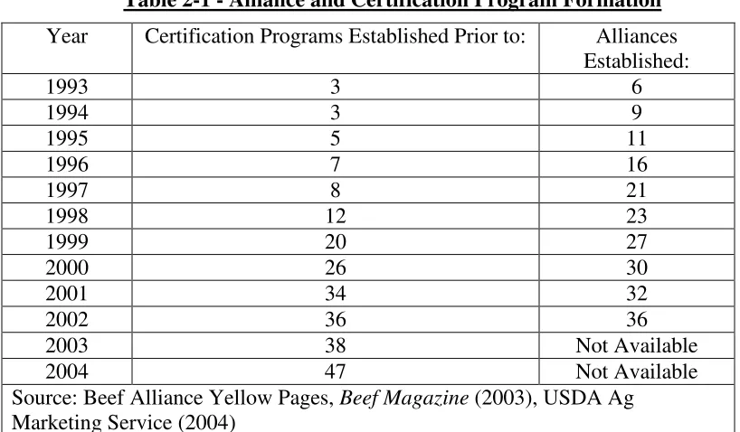
Table 2-1 - Alliance and Certification Program Formation………..40
Table 2-2 - Summary Statistics on Beef Grades, Poultry and Chicken………. 41
Table 2-3 - Summary Statistics on the Seemingly Unrelated Regression………….. 42
Table 2-4 - Estimation Results for the Gamma Parameters……….. 43
Table 2-5 - Estimation Results for the Alpha and Beta Parameters……….. 44
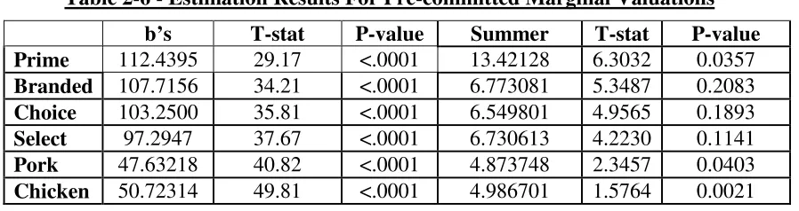
Table 2-6 - Estimation Results For Pre-committed Marginal Valuations………... 45
Table 2-7 - Estimated Compensated Cross Quantity Flexibilities………...46
Table 2-8 - Estimated Uncompensated Cross Quantity and Scale Flexibilities…… 47
Table 2-9 - Annual Benefits of Conjectured Future Increases in Branded Beef…....48
Table 2-10 - The Effect of the Introduction of Branded Beef in the 1990’s………...49
Table 3-1 - Summary Statistics on Weekly Output of Beef Grades………....94
Table 3-2 - Certification Program Formation………... 95
Table 3-3 - Index of Notations for Supply……….………. 96
Table 3-4 - Index of Notations for Demand……….……….. 97
Table 3-5 - Welfare Measures and the Number of Producers……….……….. 98
Table 3-6 - Welfare Measures and the Grade 4 Standard……….…….... 99
Table 3-7 - Welfare Measures and the Grade 4 Standard……….…….... 100
LIST OF FIGURES
Figure 2-1 - Percentage of the Commercial Slaughter Certified…….………. 50
Figure 2-2 - Market Shares of Goods Vertically Differentiated by Quality……….. 51
Figure 2-3 - The Distance Function in Quantity Space………... 52
Figure 2-4 - The Expenditure Function and Compensating Variation……….. 53
Figure 2-5 - The Distance Function and Compensating Variation………... 54
Figure 3-1 - Percentage of the Total Commercial Slaughter Certified………. 101
Figure 3-2 - Market Shares when the Error Distribution is Uniform………... 102
Figure 3-3 - Production of Grades when the Production Error is Normal……..…. 103
Figure 3-4 - Market Shares and Consumer Preferences………... 104
Figure 3-5 - Producer Surplus and the Number of Producers……….. 105
Figure 3-6 - Total Surplus and the Grade 4 Standard……….. 106
Figure 3-7 - Producer Surplus and the Grade 4 Standard……….……... 107
Figure 3-8 - Consumer Surplus and the Grade 4 Standard……….. 108
Figure 3-9 - Total Surplus and the Introduction of a New Grade……….109
Figure 3-10 - Producer Surplus and the Introduction of a New Grade……… 110
Figure 3-11 - Consumer Surplus and the Introduction of a New Grade…………... 111
Figure 3-12 - Total Surplus and the Introduction of a New Grade……….……….. 112
Figure 4-1 - Expected Qualities under Sorting……….. 144
Figure 4-2 - The Division of Consumers under Sorting………..…….. 145
Chapter 1
Agricultural production is uniquely subject to random processes influencing both the quantity and quality of output. While economic models of agricultural markets often control for shocks affecting the quantity demanded or supplied, variation in product quality is often disregarded either because data aggregation prevents the consideration of quality differences across goods or because agricultural grading is presumed to eliminate significant quality variation. In recent years, however, agricultural producers have become increasingly focused on crafting agricultural products for final consumption in retail markets rather than merely producing commodities of a predetermined quality. Often, products are branded to distinguish their unique features and marketed to more specific consumer groups. This process, often referred to as “the industrialization of agriculture,” typically requires improved quality control mechanisms and coordination of the supply chain which may be achieved through contracting and other vertical
production relationships.
principal-agent models of production are useful in addressing supply processes characterized by randomness in quality.
The first essay, “The Welfare Benefits of USDA Beef Quality Certification Programs,” estimates the consumer welfare benefits from the increase in scope of USDA beef quality certification programs in the 1990’s. Certification programs provide
producers a new way to differentiate the quality of beef products outside the USDA grading program and enable the branding of beef. Certified and branded beef essentially represents a new good with a quality level between that of the Prime and Choice grades. An Inverse Generalized Almost Ideal Demand System (IGAIDS) is estimated using weekly data on beef consumption by grade, branded beef, chicken and pork. The compensating variation from the introduction of branded beef since 1993 is then estimated to have increase consumer welfare by 1.6% of wholesale beef expenditure. The essay also examines whether demand is vertical differentiated by quality grades.
Unlike the USDA grading program, quality standards under certification
Quality differentiation through grading and certification may not be possible when quality characteristics are not observed by sellers. Goods, such as fruit and produce, may exhibit quality characteristics at the time of purchase that consumers can observe, but are unknown to sellers. In this setting, consumers have an incentive to sort goods for quality. The third essay, “When is Fruit Bundling Fruitless?” considers the conditions in which sellers allow sorting and discourage it through mechanisms such as bundling. Agricultural goods often vary in quality even when goods are sold at a single price which encourages consumers to sort goods. Consumers can increase their
Chapter 2
The Welfare Benefits of
I. Introduction
Between 1975 and 1999, beef demand fell by 66% (Marsh, 2003) and its share of the overall meat market fell from 48% to 32%. Along with changing consumer
preferences and heightened health consciousness, poor quality assurance has been offered as a reason for the decline (Lusk et al., 2001; Lamb and Beshear, 1998; Purcell, 1999). In recent years, packers and producers have introduced quality improvement mechanisms including expanded contracting, value-based pricing, and certification to capture potential gains to quality improvement. In doing so, producers branded and differentiated a good that had previously been marketed as a commodity, with the USDA acting only as a third party verifier of quality claims. Between 1994 and 2002, the share of all commercial cattle that were certified rose from 4% to 12% and the share that were both certified and qualify as upper Choice rose from 3% to 8%. While several studies have considered the impact of quality improvement in terms of producer profitability, few have sought to quantify its value to consumers.
20% is predicted to have a modest, but not statistically significant, impact on consumer welfare. Additionally, the model is tested for evidence of a vertically differentiated demand structure through tests of the substitution parameters with mixed results.
II. An Overview of the Beef Industry
Historically, beef quality has been distinguished only by the USDA grading program. Developed in the 1930’s, this voluntary federal program separates beef into eight grades based on observable characteristics of the carcass at the time of slaughter. Typically, only three or four of these grades – Prime, Choice, Select, and Standard (in order of decreasing quality) - are available in the consumer markets. Prices of graded beef are well ordered with Prime being the most expensive and lower grades costing less.
Evidence that the USDA grading program poorly measured important quality characteristics and that consumers would pay significant premiums for quality improvement led producer alliances to brand beef using USDA quality certification programs. In these programs, additional observable quality characteristics are measured by USDA graders in addition to those of the regular grading program. For example, under the Certified Angus Beef™ program, cattle must have a hide 51% black in color, show no signs of Brahman genetics, have a yield grade of 3.9 or lower, and quality for the upper Choice grade or better.
As shown in Figure (1), the number of certification programs and participation in these programs grew steadily in the last decade as the proportion of cattle certified rose from approximately 4% to 13% between 1994 and 2002.1 In that same period, the
percentage of commercial US cattle certified that also graded as upper Choice, a requirement for many certification programs, rose from approximately 3% to 8%. In
2002 and 2004, the USDA’s Agricultural Marketing Service (AMS) cutout reports showed that 7.4% of boxed beef was branded2.
Under the quality grading system, USDA graders assess both the maturity of the animal and the fat marbling of the meat flesh as younger cattle with more uniform marbling are thought to be superior. In the 1990’s, several meat science studies, including the National Beef Quality Audit (1995) showed that grading does not
distinguish3 key quality characteristics including tenderness4. Savell et al. (1987) found that USDA grade standards are ineffective at identifying meat tenderness. Wheeler, Cundiff and Koch (1999) found that only 5% of the variation in palatability traits is explained by the degree of marbling in beef, the dominant USDA grading criterion. Brooks et al. (2000) corroborates Wheeler’s results in finding that the USDA grade had no effect on tenderness of top loin steaks as measured by Warner Bratzler Shear5 (WBS) force values.
Evidence also showed that consumers are willing to pay significant premiums for improved quality of their beef purchases. Shackelford et al. (1999) find that 89% of consumers would definitely or probably buy certified “tender select” beef if it were available at their local store. Boleman et al. (1997) found that approximately 95% of consumers are willing to purchase the highest tenderness level offered as certified by the
2 The definition of branded beef by the AMS is beef that is “produced and marketed under a corporate
trademark or under one of USDA’s certified programs where the base of the brand is quality, yield, or breed characteristics of the product which are not unique to any one packer and can be produced by anyone in the industry, regardless of the brand.” On cutout reports, the AMS further explains that branded beef only includes that which also qualifies for the upper Choice category. Slight disparities between the percentage of beef certified and branded are present in the data and may arise because certified cattle are typically smaller than other cattle.
3 Grading is found to be consistent, however, as the USDA reports a 95% agreement rate across
independent evaluations.
4 Dikeman (1987) and Miller et al. (1995) show that tenderness is the most important palatabilty attribute of
beef.
WBS method when offered selection of three products of increasing tenderness and price differentials of $1.10/ kg. Lusk et al. (2001) found that 20% of consumers were willing to pay more than $2.67 more for a steak that was certified as tender using the WBS method and that 51% of consumers were willing to pay a premium for steaks “guaranteed tender" using this method. Several studies6 have also suggested that the steady erosion of beef demand from 1975 to 1999 is explained, at least in part, by the decline in the quality of beef relative to other meats.
In the 1990’s, producer alliances proliferated to capture these large potential returns7 by using certification programs to collectively market branded products as shown in Table (1). Grid pricing was developed to create incentives for producers to invest in quality improvement. As several authors have noted (Schroeder et al., 1998; Fuez, 1995), as producers have historically sold cattle on a live- or dressed-weight basis (Schroeder et al., 2002), their compensation is based on average cattle quality across all producers. A moral hazard problem emerges as producers ignore quality improvement in the pursuit of cost reduction by selecting only animals with fast growth rates, above-average feed conversion ratios, and high tolerances to weather and disease stress. Under value-based pricing, quality is explicitly incorporated in compensation as producers receive bonuses or discounts for specific animal characteristics measured at the time of slaughter. For example, under grid-pricing meat packers discount cattle with large humps, a
characteristic of exotic (Brahman) cattle, or with too much or too little fat cover.
6 Purcell (1999); Schroeder, Ward, Minnert and Peel (1998); and Lamb and Breshear (1998)
7Still, as late as 2000, Boland and Schroeder write “...at the present time, there is no value-based marketing
Certification and branding also provides a solution to an asymmetric information problem between buyers and sellers when beef is marketed as a commodity. As shown in Rosen (1976), if quality characteristics are observable at the time of purchase, those characteristics are supplied up to the point where marginal value equals marginal cost. If quality characteristics are not observable, however, the moral hazard problem reduces investment in quality especially if it creates significant opportunity costs, such as lower yields or increased herd mortality. Similarly, Holmstrom and Milgrom (1991) show that if two outputs are negatively correlated – quality and size – while only one output has a market incentive, then the output with the incentive crowds out the output with no
incentive. By improving quality assurance, the efficient supply of quality investment is a more likely market outcome.
Certification involves ex post testing of final carcass quality characteristics. In lieu of vertical integration, producers may also increase quality assurance using process verification programs. Under process verification programs, the USDA provides third party verification of specific production practices proscribed ex ante by processors. These programs are not common in US beef production8 as the small scale and long production lags at the rancher stage inhibit the writing of contracts that cover all possible contingencies, though they are common in poultry and hog production. Purcell and Hudson (2003) also note the specific problem of price volatility in the production chain has made cost-based compensation plans unworkable.
8 Lawrence (2002) explains that process verification type programs are much more common in Australia
To improve quality assurance, packers have increasingly used production
contracts9 with producers in which cattle are committed to be delivered to the packer at a specific time and may also be committed to some form of value-based pricing system. While beef has been the slowest to adopt production contracting compared with pork and poultry (Hayenga et al., 2000), evidence from Schroeder et al. (2002) suggest that it is now on the rise. Their survey of cattle producers finds that 52% of sold cattle through some sort of production contract in 2001 and that 65% expected to use production contracts by 2006.
III. Research Questions on Welfare and Demand
Three separate research questions address certification’s effect on the beef industry. The first asks, “What was the value to consumers from the introduction of branded beef?” A counterfactual analysis is performed to estimate the compensating variation that maintains the current utility level (with current prices) while adjusting relative quantities to be equal to the approximate levels of the early 1990’s. Upper Choice certification programs encompassed approximately 3% of U.S. slaughter in 1994 whereas in 2002 they encompassed over 8%. Conservatively, this suggests that branded beef supplies were at least 50% lower in the early 1990’s than today. Unfortunately, because data on branded beef was not collected prior to 2002, this can only be an
approximate figure. However, several factors–the large literature on the quality problem, the small number of certification programs, the small volumes of cattle certified, and the small number of alliances–suggest that the portion of branded beef was considerably smaller in the early 1990’s than today. To account for this inexactness, several
estimations are performed where the supply of branded beef is reduced by 10%, 20%, and
50%. In each estimation, the decrease in branded beef is accompanied by commensurate increases in the supplies of the two nearest quality grades, Choice or Prime. In this manner, the estimation strategy only examines the change in relative qualities while leaving the total supply of beef fixed.
Unfortunately, only aggregate data on branded beef and grades is available. This aggregation necessarily obscures some important quality distinctions as it lumps together “good” certified beef with “bad” certified beef. Two facts, however, mitigate this
concern. First, that approximately half of certified beef occurs under the CAB™ program. Second, that the AMS only reports beef as branded if it grades in the upper two-thirds of the Choice10 grade. A separate problem emerges, however, if the
introduction of branded beef lowers the average quality of the remaining beef sold in the Choice grade. The introduction of the intermediate grade of branded beef essentially truncates the distribution of Choice beef and reduces its quality as shown in Chapter 3 of this dissertation. Unfortunately, the lack of disaggregated data on the hedonic
characteristics of beef grades prevents the consideration of whether the introduction of an intermediate grade changes the average quality within grades.
A second research question asks, “How much will the expected future expansion of certification programs increase consumer welfare?” In the last decade, the supply of upper Choice certified beef increased an average of 13.4% annually suggesting that a 20% increase in branded beef supplies is plausible over several years. Similarly, Schroeder et al. (2002) survey cattle producers and find that that 62% expect to market
10 The upper two-thirds of the Choice grade refers to Choice graded beef with moderate marbling scores, as
cattle through a value based pricing system in 2006 versus 45% who did in 2001, though not all cattle marketed under value-based pricing are necessarily branded. To account for differences in conjectures about future supply changes, several scenarios for increases in branded beef supplies –5%, 10% and 20% increases – are simulated with the 20% increase in branded beef scenario argued as being the most plausible. Again, in each estimation, commensurate quality reductions are assumed to occur in either the Choice or Prime grades so that only the effect of shifting quality composition is estimated.
The third question asks, “Is beef demand vertically differentiated?” Vertical differentiation implies that all consumers assess quality in the same manner, but vary in their valuation of it. Beef differentiated by grade seems naturally suited to this
framework as grades are directly related to quality measurements and prices are strictly ordered. In this model, the distribution of quality valuations across consumers defines prices that clear the market for any given quantity share. Bresnahan (1987) and Greenstein (1997) have used the vertical differentiation model in a discrete choice framework to consider the introduction of new goods in the auto and computer markets respectively.
The vertical differentiation model assumes that the j goods in the market can be ranked by quality, qj, so that qj>qj-1. For instance, Prime quality is higher quality beef
than Choice beef. The variable θi is the ith consumer’s taste for quality so that larger
values of θiindicate stronger consumer preferences for quality. The indirect utility to the
ith consumer from purchasing the jth good is:
− =
purchased is
good no if 0
purchased is
good if )
, ,
( q p q p j
Consumers simply pick the good that yields the highest indirect utility or j k p q p
qj j i k k
i − ≥θ − ∀ ≠
θ (2)
The condition expressed in Equation (2) (along with the condition that consumers only
pick a good yielding a positive ij) defineθ j, the boundaries of consumer type that are
still high enough so that they purchase the jth good, in the equations below.
j j j j j j j j
j q q
p p p q p q − − = < − < − + + + + + 1 1 1 1
1 θ θ θ
θ (3)
1 1 1 1 − − − − − − = > − > − j j j j j j j j
j q q
p p p
q p
q θ θ θ
θ (4)
The distribution of across consumers defines the market share for each good with the
probability mass of the range between (θ j,θ j+1) defining the market share of the jth good.
If f( , ) is the distribution of consumer preferences dependent on other variables such as
income, age, and other demographics, then the quantity shares of each grade are
displayed graphically in Figure (2). The market share of each grade multiplied by the
number of possible consumers determines the quantity demanded of each grade.
Since the θ j determining market shares are only influenced by the prices of
adjacent goods in terms of quality, a testable implication of the vertical differentiation
model is that the cross price elasticities between non-adjacent goods are zero. In terms of
beef demand, a change in the price of branded beef would influence the demand for either
Prime or Choice beef but not Select.
VI. Literature Review on Demand Estimation and Welfare Analysis
Because quantities rather than prices of agricultural goods are fixed in the short
demand models (Barten and Bettendorf, 1989; Eales and Unnevehr, 1994; Eales, 1996;
Eales, Durham, and Wessells, 1997; Beach and Holt, 2001; and Moro and Sckokai,
2002). Agricultural products, including beef, exhibit long lags between initial production
and actual harvesting of the good. Moreover, fresh beef is perishable so that supplies
cannot be easily stored. Hicks (1956) argues that, in contrast to consumer level demand
where prices are likely to be viewed as fixed in the short-run, quantities are fixed in the
short run at the market level. Functionally, the difference between imposing price or
quantity exogeneity amounts to the difference between whether prices are the
side independent variables in an ordinary demand system or quantities are the
right-hand-side independent variables in an inverse demand system.
Importantly, demand parameters are inconsistent when the exogeneity assumption
is misplaced (prices are assumed to be exogenous when they are not or quantities are
assumed to exogenous when they are not). As Thurman (1986) emphasizes, a priori
assumptions regarding the supply adjustment process have often been imposed
haphazardly as the maintained hypothesis without consideration of empirical evidence
that might suggest a specific functional form. Thurman advises testing for either quantity
or price exogeneity using the Wu-Hausman test. In this technique, demand parameters
are first estimated using the instrumental variables (IV) method that is asymptotically
unbiased but inefficient. Demand parameters are then re-estimated using reduced form
methods assuming that either prices or quantities are exogenous. The IV and ordinary
demand estimates are identical if prices are exogenous and this property can be tested
using a Wu-Hausman test. Quantity exogeneity is tested in an identical manner. If both
should proceed with IV estimation. Non-rejection of either price or quantity exogeneity,
however, may be the result of a low power for the test and does not provide unqualified
evidence of price or quantity exogeneity and the choice of appropriate demand model
ultimately reverts to the a priori beliefs of the econometrician.
The method suggested by Thurman is infrequently implemented due to the
difficulty of obtaining appropriate instruments that are correlated with shifts in supply but
not demand. Assuming exogenous supplies in the short run seems appropriate given the
nature of beef production. Beef production is produced with extremely long lags. Cattle
reach the market 24 months after an initial calving decision and cows can produce at
most one calf per year.11 Poultry and pork have a shorter breeding cycle (4 to 6 months for pigs, 6 to 8 weeks for chickens) and the higher fertility rates so that supply may be
more responsive to price in those industries.12
The quantity exogeneity assumption also implies that producers cannot convert
low quality cattle into high quality cattle in the short run in response to price changes.
This condition is likely to rely significantly on whether high quality cattle are the product
of genetic selection (using Angus rather than Brahman genes) or higher quality inputs
(extending the feeding times of cattle). If genetics drives quality differentiation, then
exogenous quantities of cattle differentiated by grade is plausible. If inputs drive quality
differentiation, then exogenous prices are likely to be more common. Little empirical
evidence is available on this subject with the exception of Norwood and Lusk (2003,
page 14) who find a statistically significant short-term elasticity of technical substitution
11 Supply may be somewhat more responsive in that period however as heifers may be slaughtered rather
than kept as breeding cows in response to high prices. Similarly, cattle slaughter may be delayed or hastened depending on market prices although constraints on feedlot capacity prevent excessive delay.
of 2.7 for wholesale supplies of Choice and Select beef. At the same time, this
magnitude of substitution is likely to be smaller between other adjacent qualities of beef
such as branded beef and Choice graded beef due to the more rigorous genetic
requirements of the branded beef programs.
As a separate issue, measurements of welfare change only apply to wholesale
rather than retail level effects when using disappearance data rather than consumption
data as with the estimation used here. Changes in wholesale supply cannot be used to
extrapolate to changes in welfare at the retail level. As Brester and Wohlgenant (1993)
show, estimates of own-price retail demand elasticities based on disappearance data are
inconsistent because they impose the restrictive assumption that wholesale beef and
processing inputs are used in fixed proportions in producing the final retail product. If
retailers respond to more expensive beef by using beef more efficiently by increasing
processing inputs rather than reducing their beef purchases, then some of the retail level
welfare losses from restricted supply are dissipated through input substitution. As the
ability to substitute processing inputs for beef inputs in production increases (i.e. the
marginal rate of technical substitution increases), retail demand for wholesale beef
becomes more elastic. The disparity between retail and wholesale demand elasticities
prevents the results of this paper from being generalized directly to consumer level
effects.
Under the assumption of quantity exogeneity, an Inverse Generalized Almost
Ideal Demand System (IGAIDS) model of demand is used to estimate reduced form
demand parameters of an inverse utility function. Parameters are estimated using budget
generalized ordinary demand models, consumer expenditure is decomposed into two
parts, pre-committed and supernumerary expenditure. Pre-committed expenditures are
the fixed proportions of a consumer’s budget devoted to specific goods in the demand
system whereas supernumerary expenditure represents the remaining, unallocated budget.
In ordinary demand systems, once pre-committed expenditures are subtracted from the
consumer’s budget, supernumerary expenditures are then allocated as in ordinary
budgeting. In inverse demand systems, the intuition is similar with the exception that
expenditures are normalized by income (since only relative marginal valuations are
estimated). The distance function is decomposed into pre-committed distance and
supernumerary distance. Similarly, once pre-committed shares are subtracted from a
consumer’s expenditure, supernumerary shares are allocated from the remaining
normalized budget.
In contrast to ordinary demand systems, where differentiation of the expenditure
function yields compensated price elasticities, differentiation of the distance function in
inverse demand systems yields compensated quantity flexibilities. The distance function
gives the scale by which all quantities of all goods must be adjusted to obtain a given
level of utility. It is analogous to the cost function, which gives the amount by which
income must be adjusted to obtain a given level of utility. For instance, if a consumer is
currently consuming {q1=3, q2=4}to obtain utility 8, the distance function value of 1.1
for the utility level 10 implies that the quantity of all goods must be increased by 10%
{q1=3.3, q2=4.4} to achieve this higher utility level with the same relative quantities.
Price flexibilities give the percentage change in a consumer’s valuation of a good
positive, then the goods are q-complements as consumers value good i more with
increases in good j even while holding utility constant. Similarly, if the flexibility is
negative, then the goods are q-substitutes. Goods are inflexible if the absolute value of
their own price flexibility is less than one. In this case, a 1% increase in the consumption
leads to decrease in marginal value of that good less than 1%.
Scale flexibilities are the analogue to the income elasticities of ordinary demand
systems and represent the change in relative prices that would support a proportionally
expanded equilibrium bundle, with income normalized to one. If preferences were
homothetic, all scale flexibilities would be equal to -1. In this case, a 1% increase in
consumption of all commodities would require no change in relative prices but a 1%
increase in total expenditure. Normalized prices, prices divided by total expenditure,
must all decrease by 1% to obtain this improved bundle. In reference to homothetic
preferences, if the absolute value of scale flexibilities are less than -1 then goods are
necessities as the marginal valuation of the good is unresponsive to proportional increases
in the amount of all goods consumed. If the absolute value of scale flexibilities are
greater than -1 then goods are luxuries as the marginal valuation is very responsive to the
same proportional increases.13
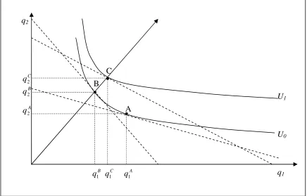
A change in a consumer’s allocation from bundle A and C can be decomposed
into two welfare effects using the distance function in quantity space in the same manner
that changes that changes can be decomposed using the expenditure function in price
space as shown in Figure (3). The first movement along the existing utility curve from A
to B, the substitution effect, shows the change in relative valuations of goods necessary to
reach a bundle of goods yielding the same utility as point A but in the same proportion as
that of point C. The second movement from B to C, the scale effect, shows the amount
that one would need to increase all the utility compensated quantities proportionally
(scale quantities) to reach the eventual allocation C.
As Cornes (1994, page 90) shows, the substitution effect and scale effects can
obtained from the compensated inverse demand curves. Assume the following identities
where i is the uncompensated inverse demand for good i and i is the compensated demand for good i.
=ζ (q,δ)
pi i pi =ζi(q,D(q,U))=ψi(q,U) (5)
Noting that the derivative of the distance function is equal to uncompensated inverse
demand, Cornes (1994) shows that Equation (5) can be used to derive the following
expressions:
(
ζ δ)
ζ ψ
ζ ∂ =∂ ∂ − ∂ ∂
∂ i qj i qj i i (6)
Multiplying Equation (6) by qj/pi yields Equation (7)
i i i j i i i j j i i j j i p p p q p q q p q q δ δ δ ζ ζ ψ ζ ∂ ∂ − ∂ ∂ = ∂ ∂ (7)
For small changes in quantities, pi, i and i are equal to each other at the optimum and is equal to 1.
j i i i i j j i i j j
i q pq
q q q ∂ ∂ − ∂ ∂ = ∂ ∂ ζ δ δ ζ ψ ψ ζ ζ (8)
The Slutsky equation can be represented in terms of quantities or elasticities. Equations
(7) and (8) are the inverse demand analogoues to the Slutsky Equation in price and
flexibility form.14 Equation (7) states that the effect of an increase in the quantity of good
14 Setting equal to one allows the p
i qi term to be interpreted as an expenditure shares. Expenditures
j on a consumer’s valuation of good i is equal to the change that results when the distance
function is adjusted (quantities of all goods are changed) so that the consumer achieves
the same utility minus the valuation of good i multiplied by the amount changing the
distance function influences the valuation of good i. Equation (8) is slightly more
manageable as it implies that the uncompensated flexibility is equal to the compensated
flexibility minus the scale flexibility multiplied by consumer expenditure on that good.
The form of the supernumerary distance function is the IAIDS model described
by Eales and Unnevehr (1994). This model exhibits many desirable properties that
mirror the ordinary AIDS model including (1) derivation from a well defined preference
structure (specifically, a logarithmic distance function), (2) flexibility in that the IAIDS
preference structure can be interpreted as a local second-order approximation to an
unknown preference structure, and (3) ease of imposition of homogeneity and symmetry
conditions. The IAIDS model is sometimes further augmented to increase its flexibility
and tractability. For instance, a shortcoming of the IAIDS model is its imposition of
linearity in the scale curves that Beach and Holt (2001) describe as the analogue to
imposing quasi-homotheticity in a direct demand system. In separate work, Beach and
Holt (2001) develop the Normalized Quadratic Inverse Demands – Quadratic Scale
System to incorporate quadratic terms into scale curves while Moro and Sckokai (2002)
derive the Inverse Quadratic Almost Ideal Demand System (IQUAIDS).
Alston, Chalfant and Piggott (2001) show that in many empirical estimation
strategies, the IAIDS (and ordinary AIDS) model estimates of real variables (such as
market shares, elasticities or flexibilities) are sensitive to the choice of scaling of the
version of the AIDS and IAIDS models, first developed by Bollino (1987), preserve the
desirable theoretic property of being ‘Closed Under Unit Scaling’ (CUUS). As shown
by Piggott and Marsh (2004), a generalized expenditure function is defined as follows:
) , ( ~ )
,
(p u p c E p u
E = ⋅ + (9)
The first right-hand-side term represents pre-committed expenditures (prices, p,
multiplied by pre-committed quantities, c) while the second term represents
supernumerary expenditure.
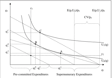
Figure (4) shows the effect of an exogenous decrease in the price of q2. The
variables c1 and c2depict pre-committed quantities. The movement from A to B captures
the substitution effect. The movement from B to C captures the income effect. The q1
axis intercepts multiplied by p1 give the expenditure function for a given level of prices
and utility and their difference is the compensating variation.
Invoking duality, a generalized distance function is similarly expressed in terms
of pre-committed and supernumerary expenditures with the exception that the distance
function is depicted in (normalized) price space. The generalized distance function is
then written as:
) , ( ~ )
,
(qU q b D qU
D = ⋅ + (10)
Again, the distance is decomposed into pre-committed and supernumerary components.
The b terms represent pre-committed relative marginal valuations. The distance function
assumes that relative prices are endogenous and adjust in response to exogenous changes
in quantities. Figure (5) depicts an exogenous shift from A to C in price space. Here, the
amount of q1 increases relative to q2. The shift from A to B shows the change in relative
prices proportionally so that consumers attained the same original utility. The norm (the
slope from the ray emanating at the origin) to A is the price ratio (p2/p1). The norm to B
and the norm to C are equal because they both represent a rescaling of the same relative
prices. Moving from A to B indicates that the marginal valuation of q2 increased relative
to q1. The slope of the tangent to the indirect utility curve is the ratio of quantities
consumed at optimum for given levels of utility. Given that prices are normalized, the
move from B to C shows the proportional decrease in all prices to reach the higher utility
level at C while maintaining the same relative prices as B. Rescaling all prices
proportionally is equivalent to rescaling all quantities proportionally. For this reason, a
parallel downward shift in the tangent of B so that it intersects C creates a new
intersection point to the p1axis. This point gives the normalized expenditure (at the
original prices) required to obtain utility C. The difference in normalized expenditure
from the line intersecting B and the line intersecting C represents the compensating
variation in normalized prices. The distance function is equal to the intercepts to the p1
axis in the same manner that the expenditure function (normalized by p1) is equal to the
intercepts of the q1 axis. The distance function is typically characterized as the rescaling
of all quantities necessary to obtain the same utility from a price level B as that at price
level C. The rescaling is identically depicted as the rescaling of intercepts to the p1 axis.
As with the quantity dependent AIDS model, pre-committed marginal valuations
can be incorporated into the demand model and estimated in empirical settings. The
intuitive interpretation of committed marginal valuations is not as transparent as
pre-committed quantities in ordinary demand estimation. Pre-pre-committed quantities are
function structure. There is no comparable interpretation of pre-committed marginal
valuations.
V. Description of the IGAIDS Model
Estimating the IGAIDS model involves simultaneously estimating the
pre-committed and supernumerary distance as in Equation (10). The supernumerary
component of the distance function is estimated using the Inverse Almost Ideal Demand
System as shown by Eales and Unnevehr (1994) which is derived from the logarithmic
distance function: ) ( ln ) ( ln ) 1 ( ) , ( ~
lnDU q = −U a q +U b q (11)
Components of the supernumerary distance function are then given as:
+ +
= j qj ij qi qj
q
a( ) ln ln ln
ln 21
0 α γ
α (12) ) ( ln ) (
lnb q 0 q a q
j j
j +
=β
∏
−β(13)
According to Antonelli’s identity, differentiation of the regular distance function yields
compensated inverse demands; Similarly, differentiation of the logged distance function
yields compensated share functions, which are budget shares as function of quantities of
all goods and utility. Compensated share functions can be converted to ordinary share
functions by substituting the utility function into supernumerary distance function.
Defining supernumerary expenditure as M~ =M − iqibi, the share equations are:
( )
q Mw M M M b q
wi i i ~i , ~
~ +
= (14)
is supernumerary, multiplied by w~ , good i’s share of supernumerary expenditures. Each i
good’s compensated share of supernumerary expenditure is:
∏
− + + + = j j ij ij j
j j
i i q q U q j
w~ α α ln γ ln β β0 β (15)
Recalling that lnD(U,q)equals zero at the optimum and isolating for
∏
−j j
j
q
Uβ0 β allows one to solve for the uncompensated share equations of:
+ +
+ +
=
k l kl k l
k k k
i
j ji j
i
i logq logq logq logq
~
2 1
0 α γ
α β γ
α
ϖ (16)
Substituting w~ into Equation (14), the estimated share functions are: i
+ + + + + =
k l kl k l
k k k
i
j ji j
i i
i
i M q q q q
M M b q log log log log ~ 2 1
0 α γ
α β γ
α
ϖ (17)
Because 0 is not identified through the budget shares in Equation (17), it is set to one
throughout the estimation15. Pre-committed marginal valuations include a seasonal demand shifter, s, for the summer months so that bi =bi +di×s
~
. Alston, Chalfant, and
Piggott (2001) show that specifying a demand shift in this manner preserves the CUUS
property.
As found with previous studies estimating the AIDS and IAIDS model, the 0
parameter is difficult to estimate. Deaton and Muellbauer (1980) explain that the 0
parameter can be interpreted as the “outlay required for a minimal standard of living
when prices are one.” As the estimated model did not converge when 0was included in
the model, this paper followed the practice of previous authors (see Eales and Unnevehr,
1994) by setting 0to zero a priori. Convergence is likely to have failed because the
15Equation (22), later in the paper, shows that the
0term is a scalar on utility which can be changed
likelihood function is flat over a substantial range of 0 values. An alternative method of
estimating the model without omitting 0 is described by Piggott (1997). A grid search is
performed where 0 is set to a range of possible values. In each case, the model is
re-estimated treating the 0 term as constant. The value of the likelihood function at the
alternative 0values is used to rank the different model specifications. Finally, the
model is re-estimated using the 0value with the largest likelihood value as the starting
point for 0 in estimation. Convergence might occur because the 0 value begins near a
local optimum.
Other restrictions drawn from economic theory are imposed including:
=
k k
1
α , =0
k k
β , (Adding Up) (18)
=
k jk
0
γ (Homogeneity) (19)
j i ji
ij =γ ∀ ≠
γ (Symmetry) (20)
Adding up restricts supernumerary distance to equal one which implies that
supernumerary expenditure shares sum to one. Homogeneity restricts proportional
increases in all prices and income to have no influence on the supernumerary expenditure
shares. Symmetry restricts the compensated flexibilities of good i and good j to equal the
compensated flexibility of good i on good j within supernumerary expenditures although
compensated flexibilities are no longer symmetric for all expenditure. When
compensated flexibilities are estimated for total expenditures, symmetry no longer holds.
The restrictions resulting from vertical differentiation can also be imposed and
tested with the follow restrictions:
0 =
ij
Vertical differentiation implies that only goods of adjacent qualities act as substitutes.
For instance, Prime beef would not be a substitute for Select, for example. A test of this
restriction is whether the between Prime (where i = 1) and Select beef (where i = 4) are
zero and, in general, whether the ’s between non-adjacent quality levels of beef are zero.
Unfortunately, this specification only restricts the substitution parameters within the
supernumerary expenditures. It is not possible to impose a marginal rate of substitution
equal to zero between two goods in the IAIDS model without severely constraining the
scale flexibilities.16 The problem arises from the specification of utility in the inverse
AIDS model. Noting that the distance function is equal to one at the optimum, utility is
represented as: j j j j i ij j j q q q q U β β γ α −
∏
+ = 0 21 ln ln
ln
(22)
Notice that this specification implies that an adjustment in qj will still affect the marginal
utility of qi through the j term in the denominator even if the ij between two goods is
zero. This specification puts a strong bias against finding zero cross-quantity flexibilities
if any substantial scale effects (captured in the i’s) exists.
For the IGAIDS model, equations for the compensated, uncompensated and scale
flexibilities are:
Uncompensated Own Quantity Flexibility (fij)
(
−)
+ − + + + − = = j N j ij i i i i ij i i i iij M q
b q M w b q Mw
f 1 1 1 ~ ln
1
γ α
β
γ (23)
Uncompensated Cross Quantity Flexibility (fij)
16 Similarly, a parameter restriction cannot be defined which imposes the scale flexibility of a good to be
(
−)
+ − + + = = j N j ij i i i i ij i i i iij M q
b q M w b q Mw
f 1 1 ~ ln
1
γ α
β
γ (24)
Scale Flexibility (fi)
(
−)
− + + + − + = = j N j ij i i i i ij i ij M q
b q M M b q M
f 1 1 ~ ln
1
γ α
β
γ (25)
Compensated Flexibility ( h)
ij f j j ij h
ij f w f
f = − (26)
The compensating variation17 is a well-established measure of consumer welfare effect resulting from changes to price or quantity (See Chapter 7 of Deaton and
Muellbauer, 1998 for discussion). With ordinary demand systems, the compensating
variation is typically calculated as the change in the expenditure function, the cost of a
consumer reaching a utility level at a given set of prices. With inverse demand systems,
however, the compensating variation is calculated the change in distance function from a
quantity shift multiplied by income. As discussed in Kim (1997) and Beach and Holt
(2001), the compensating variation is as follows:
(
) (
)
(
0 1 0 0)
0 Du ,q Du ,q
M
CV = − (27)
As Figures (5) and (6) show, the distance function is analogous to the expenditure
function of ordinary demand systems. Once re-scaled by income, M0, the distance
function equals the cost of reaching a given utility level with different proportions of
goods. Holding utility constant, the difference in distance at different quantities
multiplied by income gives the compensating variation of a quantity change.
17 The difference between the two measures is whether utility is held constant at its initial level or its final
VI. Description of the Data
The described demand system is estimated with 108 weekly observations of
prices and quantities of four grades of beef (Prime, Choice, Select, and Ungraded, in
order of quality), branded beef, pork, and chicken between January 1st 2002 and January 30th 2004. Summary statistics of the data are provided in Table (2). Beef prices are the total carcass values of different grades of beef; Beef quantities are computed from total
wholesale loads (40,000 pound shipments) from packing plants.18 Both values are publicly available from the Agricultural Marketing Service Branch of the USDA weekly
price reports made available after the passage of the Mandatory Price Reporting Act of
1999. Pork and chicken data are obtained from the Livestock Marketing Information
Center. Pork prices are based on total carcass cutout values and quantities are based on
dressed weights. Chicken prices are the 12-city broiler price and quantities are the total
live-weights of chickens. Chicken weights are adjusted to reflect dressed weight
quantities by multiplying by 0.71, the approximate dressed weight to live weight ratio of
chickens reported by the USDA National Agricultural Statistics Service19 (2004). Quantities are in millions of pounds and prices are in cents per pound.
Notably, Prime graded beef is a small proportion of total beef expenditures and
exhibits little variation in quantity. Chicken and pork represent roughly 40% and 25% of
consumer meat expenditures. Collectively, beef represents the remaining 35% of
consumer expenditure with the Choice, Select and Ungraded categories representing the
largest portions of beef. The price difference between Select and Ungraded beef is small
18 There are certain exemptions for reporting to small packing plants which represent a small portion of the
market.
19 The actual ratio is obtained by dividing pounds of broilers certified as ready to cook by live weights. In
and the prices are very closely correlated. For this reason, Ungraded beef is excluded
from the estimation of the remaining demand system.
The data appears consistent with outside sources. Using the 2000 U.S. Bureau of
Census estimate20 of a US population of 281 million, the average total expenditure on wholesale chicken, pork and beef in the US is approximately $150 per year. The
Consumer Expenditure Survey of the Bureau of Labor Statistics21 estimates that average consumer expenditure of chicken, pork and beef to be $542 dollars but this figure should
be discounted by approximately 40% to account for the wholesale-retail price spread22
and then further discounted to account for the role of imports.
VII. Estimation Results
The demand system was estimated by fitting Equation (17) for the three beef
grades, branded beef, and pork and chicken as a seemingly unrelated regression using the
PROC MODEL function in SAS, which jointly estimates the shared parameters of the
demand system while weighting the errors of the share equations by the inverse of the
covariance matrix. The dummy variable for the summer month is defined as those weeks
of the summer between the last week of May (Memorial Day) and the first week of
September (Labor Day). Summary statistics for the seemingly unrelated regression are
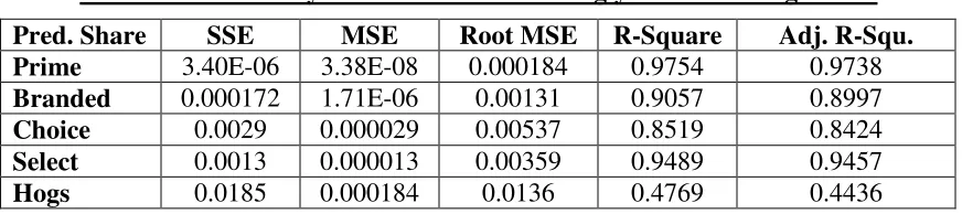
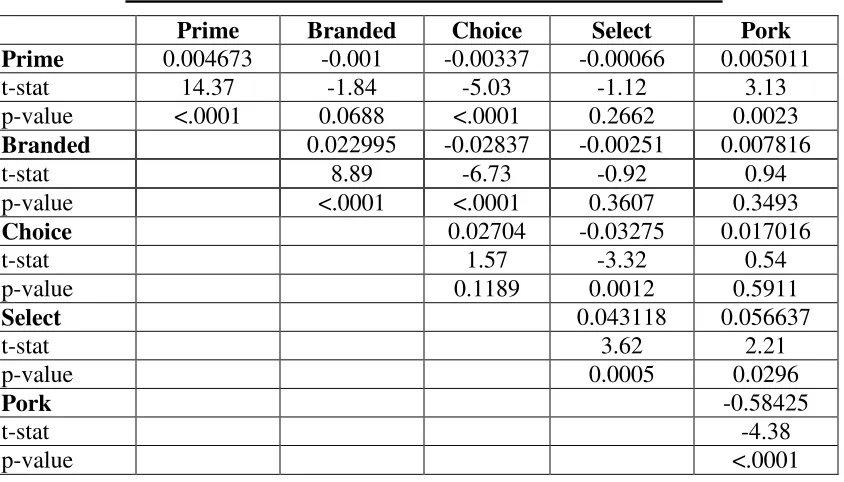
provided in Table (3). Estimates of the parameters estimated in Equation (17) are given
in Tables (4), (5) and (6) with chicken being the excluded good from estimation.
The demand model predicts well with nearly 84% of the variation in beef
expenditure shares and 44% of the variation in pork expenditure shares being explained
20Source: U.S. Census Bureau, http://eire.census.gov/popest/estimates.php 21Source: U.S. Bureau of Labor Statistics, http://www.bls.gov/ces/
22The Economic Research Service of the USDA estimated that the average per pound sale price of beef is
by the quantity variables. Gamma parameters are significant with notable exception of
those between Prime and Select and those between Branded and Select. Seasonal
variables positively impact demand but are not significant with the Branded, Choice and
Select grades. None of the parameters are significant. Evaluating the flexibility
formulas at all data points and taking the average of these estimates gives the estimates of
compensated and uncompensated flexibilities provided in Tables (7) and (8).
The scale flexibilities imply that pork and all grades of beef are luxuries while
chicken is not.23 The small (in absolute terms) own quantity flexibilities imply that the
demand elasticities are large.24 The large asymmetry between cross quantity flexibilities between chicken and pork to beef may be due to the large difference in budget shares
between those goods upon which the flexibility formulas depend. Since the cross
quantity flexibilities between each grade of beef are negative, they indicate that all beef
grades are q-substitutes for all other beef grades. So, for example, an increase in holdings
of Choice beef decreases the marginal value of Select beef.
VII.A. Vertical Differentiation
The vertical differentiation restrictions were tested by using a small-sample
likelihood ratio test25 to consider whether the gamma parameters between non-adjacent grades – Prime-Select, branded-Select, and Prime-Choice – were zero. In the first two
cases, the gamma values were not found to be statistically different from zero which
partially supports the vertical differentiation hypothesis. However, because the gamma
parameters only capture the substitution effects in the demand system, both the
23 Park and Thurman (2001) show that the weak connection between the scale flexibility and the income
elasticity prevents stronger statements from being made.
24 Beach and Holt (2003) similarly argue that small quantity flexibilities imply large elasticities due to the
reciprocal relationship between the two variables.
compensated and uncompensated cross quantity flexibilities between these goods will not
equal zero as Equations (24) and (26) indicate. Because evidence on vertical
differentiation of the demand system is mixed and to maintain flexibility in the estimation
process, the vertical differentiation restrictions were not imposed in the remaining
estimation sections.
VII.B. Potential Future Consumer Welfare Gains
To project the compensating variation from expected future increases in branded
beef supplies, several alternative assumptions are made regarding supply changes in the
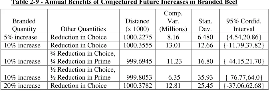
simulations. Table (9) presents conjectured future increases to branded beef supplies and
simulations of their associated compensating variations. Welfare estimates were obtained
through simulations in three steps. First, 1000 simulated draws26 on the parameters were
made given the distribution of parameters in Tables (4), (5), and (6). Second, the
compensating variation for each period was calculated using equation (27) and averaged
over periods. Finally, the standard deviation of the compensating variation for each
average compensating variation is used to construct confidence intervals for the
compensating variation.
To isolate the effect of improved quality rather than increases in the total volume
of output, each conjectured increase in branded beef is associated with a commensurate
decrease in the volume of another grade. Between 2002 and 2004, branded beef
represented approximately 7.5% of total beef expenditure and 6.8% of total beef volume.
Therefore, a 5% increase in branded beef supplies would only increase its volume share
to 7.1% while a 20% increase would only raise it to 8.2%. Between 1995 and 2002, the
26 Larger simulations using 2000, 3000, 4000and 10000 draws found similar results suggesting that
percentage increase in the number of cattle certified average 14.6% while the percentage
increase in those certified and qualifying as upper Choice averaged 2.7% of cattle. A
20% increase in branded beef supplies over 5-10 year period seems the most plausible
scenario for future supply increases. As shown in Table (2), the quantity of Prime graded
beef exhibited relatively little variation compared to other grades of beef as measured by
its small standard deviation. Moreover, because branded beef volume share is so much
larger than Prime beef, equal volume changes for each grade produce a much larger
change in the share for Prime beef. For these reason, it seems unlikely that substantial
portions of increases in branded beef supplies would be drawn from Prime beef supplies.
As Table (9) shows, a 20% increase to the supply of branded beef27 that is drawn only from Choice is predicted to increase consumer welfare by 0.0345% of total
wholesale beef expenditure or $12.807 million on an annual basis this is asserted to be
the most plausible scenario for the near future. If the change, however, is smaller and a
substantial portion is drawn from Prime beef rather than Choice beef, increased branded
beef supplies actually generate a welfare loss. In general, the potential gains from
increases in branded beef supplies are modest and not statistically significant.
VII.C. Consumer Welfare Increases in the 1990’s
Measurements of the compensating variation from the introduction of branded
beef in the 1990’s are obtained in a similar manner. Mean estimates and confidence
intervals are simulated with 1000 different random parameter draws from the distribution
of estimated demand system parameters. Again, because exact data on the aggregate
27 This change is equal to an average shift of 1.54 million pounds of production from Choice to branded on