Implementing Joux-Vitse’s Crossbred Algorithm
for Solving
MQ
Systems over
F
2on GPUs
Ruben Niederhagen1, Kai-Chun Ning2, and Bo-Yin Yang3
1
Fraunhofer SIT, Darmstadt, Germany
Eindhoven University of Technology, Eindhoven, The Netherlands
IIS and CITI, Academia Sinica, Taipei, Taiwan
Abstract. The hardness of solving multivariate quadratic (MQ) sys-tems is the underlying problem for multivariate-based schemes in the field of post-quantum cryptography. The concrete, practical hardness of this problem needs to be measured by state-of-the-art algorithms and high-performance implementations. We describe, implement, and evalu-ate an adaption of the Crossbred algorithm by Joux and Vitse from 2017 for solvingMQsystems overF2. Our adapted algorithm is highly
paral-lelizable and is suitable for solvingMQsystems on GPU architectures. Our implementation is able to solve an MQ system of 134 equations in 67 variables in 98.39 hours using one single commercial Nvidia GTX 980 graphics card, while the original Joux-Vitse algorithm requires 6200 CPU-hours for the same problem size. We used our implementation to solve all the Fukuoka Type-I MQ challenges forn∈ {55, . . . ,74}. Based on our implementation, we estimate that the expected computation time for solving anMQsystem of 80 equations in 84 variables is about one year using a cluster of 3600 GTX 980 graphics cards. These parameters have been proposed for 80-bit security by, e.g., Sakumoto, Shirai, and Hiwatari at Crypto 2011.
Keywords: Post-quantum cryptography, multivariate quadratic systems, parallel implementation, GPU.
1
Introduction
With the advent of quantum computing, an adversary can efficiently break uni-versally adopted public-key cryptographic schemes, e.g. RSA and elliptic-curve cryptography, with a sufficiently large quantum computer [16,17]. In order to mitigate this imminent threat, cryptographic schemes that are resistant against quantum computers have drawn great attention from academia. These schemes are collectively referred to as post-quantum cryptography (PQC).
One potential candidate for PQC ismultivariate cryptography. Multivariate cryptography relies on the difficulty of solving a system of mpolynomial equa-tions in nvariables over a finite field. The complexity of solving a multivariate
polynomial system (MP problem) or a multivariate quadratic system (MQ
problem) where coefficients of the monomials are independently and uniformly distributed (i.e. random) is well-known to be NP-hard. An arbitraryMPsystem can be transformed into an equivalent MQsystem by substituting monomials of degree larger than two with new variables and introducing extra equations to the system. Furthermore, a polynomial system over any extension fieldF2n can be reduced into an equivalent system overF2 using Weil descent.
Since the early 1980s, various asymmetric multivariate encryption schemes (e.g., [14,5,18]) based on Hidden Field Equations (HFE) [10] as well as signature schemes (e.g., [13,12,6]) have been proposed. Besides these asymmetric schemes, some symmetric encryption schemes, e.g., the stream cipher QUAD [1], have been proposed and analyzed [20].
Introducing a trapdoor into an MQsystem for the use in public-key cryp-tography results in a system that is not truly random and typically exhibits a hidden structure that often can be exploited in its cryptanalysis. However, we do not focus on the cryptanalysis of any particular cryptographic scheme by ex-ploiting some hidden structure. Our goal is to investigate the concrete, practical hardness of the underlying problem of solving random MQsystems overF2 by
providing an efficient, parallel implementation of the state-of-the-art algorithm. This paper is structured as follows: In Section2, we introduce the Crossbred algorithm by Joux and Vitse and our adaption to this algorithm. In Section3, we describe our implementation of the adapted algorithm for a cluster of GPUs. In Section4 we describe how to choose the parameters for our implementation, given a specificMQ system size, and in Section5, we provide an evaluation of our implementation.
The source code of our implementation and further information are available atwww.polycephaly.org/mqsolver/.
2
Joux-Vitse’s Crossbred Algorithm
There are several approaches for solving MP systems, e.g., Faug`ere’s F4 and F5 algorithms [7,8] based on the computation of Gr¨obner-bases and a family of algorithms based on extended linearization (XL) [19]. ForMQsystems overF2,
Fast Exhaustive Search (FES) [3], i.e., efficient enumeration over the search space, was the approach used by the previous record holder [4] of Fukuoka MQ Type-I and Type-IV challenges4. The record on Type-I challenges is now held
by an implementation of the Crossbred algorithm by Joux and Vitse [11]. The basic idea of the XL algorithm is to extend the originalMQsystem by multiplying it by all monomials up to a certain degree D−2 and by treating monomials in the resulting degree-D system as linear variables. Solving this linear system gives a solution for the originalMQsystem with high probability, ifD is chosen large enough.
FES works by enumerating all possible assignments of the variables and by checking the correctness of each assignment with the original MQ system. In
4
contrast to a plain brute-force search, the possible assignments are enumerated in Gray-code order such that there is only one single variable with a different assignment in each enumeration step. This allows to compute the new evaluation result efficiently based on the change in regard to the previous evaluation result, which requires storage and recursive update of partial derivatives up to the total degree of the system [4].
2.1 The Crossbred Algorithm
The basic idea of Joux and Vitse’s Crossbred algorithm is to extend the original
MQsystem to a system with a degreeD lower than the degree required for XL and to derive a sub-system that has at most degreedin the firstkvariables. This sub-system is then solved by iterating over the remaining n−k variables and solving the resulting degree-dsystem inkvariables in each iteration. Ford= 1, this requires to only solve a linear system ink variables for each assignment of n−k variables.
For example, by fixing the last two variablesx3andx4, the sub-system
S =
x1x4+x2x3+x1+x3+x4= 0
x1x3+x3x4+x2+ 1 = 0
x2x3+x2x4+x3x4+x1+x4= 0
becomes a linear system inx1andx2. Clearly, the resulting linear system can be
directly solved with Gaussian elimination, with which solutions to the systemS
can be derived efficiently. For a monomial xα = xα1
1 x α2
2 . . . x αk
k x αk+1
k+1 . . . x αn
n , the total degree of the
firstk variables is denoted as degkxα=Pk
i=1αi. Given anMQ systemF, the
Crossbred algorithm first computes a degree-D Macaulay matrix with respect to a monomial order >degkwhere monomials are sorted according to degk in descending order. Subsequently the algorithm extracts at leastkequations where the monomials of degk larger than one (which are non-linear inx1, . . . , xk) are
eliminated and only keeps monomials of degk ≤1 (which are linear inx1, . . . , xk).
These equations give a sub-system that can be transformed into a linear system in the first k variables by fixing the remaining n−k variables. After one such sub-system S is obtained, Crossbred performs exhaustive search by fixing the lastn−kvariables and testing whether or not the resulting linear systemS0 is
solvable. If so, solutions toS0 are checked with the originalMQsystemF. The
algorithm terminates if a solution is found, otherwise it fixesn−kvariables in
S with another set of values and continues the exhaustive search procedure. To obtain a linear systemS0from the extracted sub-systemS, the Crossbred
algorithm uses a recursive algorithm called FastEvaluate to fix n−k variables inS. The basic idea of this algorithm is to split each polynomial into two groups of monomials. An arbitrary polynomialpcan be written asp=p0+xip1, where
xip1 are monomials that involve a specific variable xi while p0 are monomials
Algorithm 1 The Original Crossbred Algorithm
1: procedureCrossbred
2: Input:
3: anMQsystem ofmequations innvariablesF={f1, f2, . . . , fm}
4: Macaulay degree:D
5: number of variables to keep:k
6: number of variables to fix duringMQexternal hybridization:p
7:
8: foreach (xn−p+1, . . . , xn) in{0,1}pdo
9: 1. Fix the lastpvariables inF to obtain anMQsystemF0. 10: 2. Compute the degree-D Macaulay matrix MackD
11: where monomials are sorted by degk based onF0.
12: 3. Extractrlinearly independent equationsS ={s1, s2, . . . , sr}from MackD
13: where monomials of degk>1 have been eliminated. 14:
15: CallFastEvaluate(S, k, n−p) and 16: foreach output linear systemS0
do
17: 4. Test ifS0
is solvable. If so, extract solutions and verify them withF. 18: 5. Continue if no solution is found.
19: Otherwise output the solution and terminate.
20: end for
21: end for
22: end procedure
xi = 0 in p and p0+p1 is the result of fixing xi = 1 in p. This idea can be
applied recursively to fixn−kvariables.
One can further fix some variables in the originalMQ system before com-puting Macaulay matrices, which is referred to as external hybridation by the authors [11]; here, we use the term external hybridization. The authors of the Crossbred algorithm consider external hybridization merely as a method to dis-tribute the workload between computers and do not expect it to be asymp-totically useful [11]. Nevertheless, this technique can be helpful to increase the number of variables that can be kept for linearization, which reduces the runtime of the algorithm significantly.
2.2 Adapting the Crossbred Algorithm for Parallel Implementation
The FastEvaluate algorithm proposed by Joux and Vitse has the disadvantage that computing the subsetsp0andp1on higher levels of the recursion is relatively
expensive. We propose to use Gray-code enumeration [3] instead of FastEvalu-ate, which requires only O(2n−k ·D ·k) machine instructions on the cost of
O(PD
i=0 n−k
i
·k) memory.
Gray-code enumeration was proposed to efficiently evaluate a polynomial functionf(x1, x2, . . . , xn) in all points (x1, x2, . . . , xn)∈Fn2. To obtain the result
of evaluatingf on the next pointa∈Fn2from the current resultf(a0) where only
theith coordinates ofaanda0differ,O(1) machine instructions are executed to combinef(a0) with the result of evaluating the first order partial derivative ∂x∂f
ona0 [3]. In particular,f(a) =f(a0) +∂x∂f i(a
0). This technique can be applied
recursively to evaluate ∂x∂f i(a
0) and its higher order partial derivatives until the
partial derivative reduces to a constant. Therefore, if f is of degree D, O(D) operations are required to computef(a).
The same technique can also be applied to evaluate a functionfwhose output is alinear functioninkvariables instead of a constant overF2by simply splitting
the polynomial into a sum ofk+1 sub-polynomials, one for each of thekvariables and one for a constant term. For example, the polynomial
f =x1x4x5x6+x1x4x5x7+x4x5x6x7+x1x4x5+x3x4x7+x3x5
+x2x4x6+x4x6x7+x1x4+x1x5+x5x7+x6x7+x1+x2+x4+ 1
which is linear inx1, x2, andx3can be split into the 4 polynomials
f1=x1(x4x5x6+x4x5x7+x4x5+x4+x5+ 1),
f2=x2(x4x6+ 1),
f3=x3(x4x7+x5),
f4=x4x5x6x7+x4x6x7+x5x7+x6x7+x4+ 1,
such thatf =f1+f2+f3+f4. Now,f can be evaluated by applying Gray-code
enumeration tof1, f2, f3,andf4individually.
Since the result of evaluatingf or any of its partial derivatives on a point a ∈F42 is a linear function that can be represented by four F2 elements (three
variables and the constant term) and the last order partial derivatives reduce to constants, evaluatingf(a) takes at most 3·(3+1)+1xor-operations and another 4·2 operations for computing the indices of the coordinates that changed during enumeration. In general, for a polynomial function f of degreeD whose output is a linear function inkvariables, evaluatingf requiresO(D·k) operations.
Since a machine instruction operates on machine words, which for example have size 64 for 64-bit architectures or 32 on GPUs, multiple polynomials can be evaluated with Gray-code enumeration simultaneously. Therefore, the algorithm described above can be applied to fixn−kvariables in an extracted sub-system
S ofmequations innvariables usingO(D·k) instructions, as long asmis not larger than the machine word size.
Gray-code enumeration can be easily parallelized: To run the enumeration with 2t threads in parallel, first fixt variables in the sub-system S with all
t-tuples in {0,1}t to create 2t smaller sub-systems in n−t variables. With this
approach, although the sub-systems are distinct from each other, their last order partial derivatives with respect to then−t−kvariables that must be fixed are identical.
3
Implementation
The Gray-code enumeration part of the Crossbred algorithm is particularly easy to parallelize and therefore suitable for GPU deployment. Thus, we use the CPUs to generate and process the Macaulay matrix and the GPUs for Gray-code enu-meration and linear-system solving.
3.1 Macaulay-Matrix Computations
The first step in Joux-Vitse’s Crossbred algorithm is to extend the originalMQ
system to a Macaulay matrix of degreeD. (Our implementation works forD= 3 and D= 4.) The columns are ordered such that the monomials with degk >1 are in the front. Then, several (in our implementation 32) non-trivial vectors in the left kernel of the Macaulay matrix are computed. Finally, a sub-system linear inx1, . . . , xk is extracted for Gray-code enumeration.
Since the Macaulay matrix is very sparse, a sparse-system solver like the block Lanczos algorithm or the block Wiedemann algorithm could be used. However, the Macaulay matrix exhibits a special structure: Since the Macaulay matrix is generated from the original system by multiplying the polynomials with all monomials up to a certain degree, the resulting matrix is close to being diagonal. Therefore, we decided to exploit this special structure in a specifically adapted implementation of Gaussian elimination.
The first step is to compute the reduced echelon form of the original input system. This is a very small computation and requires a negligible amount of time. Then, we compute the Macaulay matrixM such that the columns are in the required order. We store Min a sparse representation. Then we search for rows in the Macaulay matrix that have an increasing number of leading zeros and swap them into place: Find a row that has no leading zeros and swap it to the top, find a row that has one leading zero and swap it to the second row, and so on. Due to the structure of the Macaulay matrix, usually about two thirds of the rows of the upper-triangular form ofMcan be obtained just by swapping in suitable rows. Now, only the remaining one third of the upper-triangular form ofMneeds to be computed. Observe that up to this point,Mcan be stored in a sparse format and no costly row reductions needed to be performed.
In order to compute the remaining rows of the upper-triangular form ofM, one must perform row reduction. Therefore, we switch over to a dense represen-tation by first performing row reduction on rows that have not found their final position during row-swapping with those that did. In this manner, we drop those rows and columns that already have been pivoted by row-swapping and obtain a dense, reduced matrixRM. On this matrix, we perform classical Gaussian elim-ination in order to compute the desired sub-system that is linear inx1, . . . , xk.
API to distribute the workload over all CPU cores. We observed during ex-periments that our GPU implementation on a Nvidia GTX 980 graphics card outperforms our CPU version on a AMD FX-8350 4GHz processor by a factor of 9 in most cases.
Since the size of registers on a GPU is 32 bits and both Gray-code enumera-tion and linear system solving require the input system to be stored in column-wise format, only 32 linearly independent equations need to be extracted from the reduced Macaulay matrixRMfor the sub-systemS.
3.2 Fixing Variables in the Sub-system
We implemented the Gray-code enumeration algorithm for fixingn−kvariables in the degree-D sub-system S to enumerate linear systems in k variables for the GPU architecture. The data structures used by Gray-code enumeration are allocated from the off-chip global memory. We simply distribute the workload over 2t threads by fixingt variables inS to obtain individual and independent smaller sub-systemsSi,1≤i≤2tfor each thread. Since the last partial
deriva-tives are constants and remain the same for all 2t smaller sub-systems as noted in Section 2.2, they can be shared by all threads. Since they are constant, we store them in read-only constant memory.
The GPU threads in a warp begin enumeration with the same starting point and consequently they will access partial derivatives in the same order in each iteration. Therefore, the data structures for one warp can be interleaved to obtain optimal memory throughput. In addition, because of the cyclic nature of Gray-code enumeration, the last-level derivatives stored in constant memory are likely to be cached in the constant memory cache. Since the data of the 32 equations in the sub-system is stored in column-wise format, in total n−Dk−t32-bit integers are required for storing the constant last-level derivatives.
As described in Section2.2, the evaluation of a k-linear polynomial is split into the evaluation of k+ 1 polynomials. Therefore, we store the data for the non-constant partial derivatives for the 32 threads in one warp in basic units of 32(k+ 1) words interleaved in memory. Since for each of the k+ 1 polyno-mials n−k−t variables have to be fixed during enumeration, storing results of evaluating the non-constant partial derivatives ofSi requires PjD=1−1 n−jk−t
such basic memory units for one warp. Together with the result of evaluating
Si at the current point (which requires one basic unit as well) a warp requires
PD−1
j=0
n−k−t j
basic units. Therefore, in total Gray-code enumeration requires
(2t−5·PD−1
j=0
n−k−t j
)·32·(k+ 1) words of size 32-bit in global memory and
n−k−t D
words of size 32-bit in constant memory.
3.3 Testing the Solvability of a Linear System
system is small, the straight-forward approach for testing its solvability is to simply solve it with Gauss-Jordan elimination.
In the standard Gauss-Jordan elimination algorithm, once a pivot row for the ith pivot element is located, it is moved to its final position by swapping
with theith row. However, we are storing the linear system in column order, so
row swapping is expensive. Therefore, we avoid row-swapping by maintaining a mask that tracks which rows are in their final position.
After as many rows as the number of variableskin the linear systemSihave
been marked as final, the algorithms stops. The remaining unmarked rows are redundant equations and their firstk coefficients which represent the variables x1, x2, . . . , xk are guaranteed to be zero. Therefore, testing the solvability ofSi
is as simple as checking if the constant term of any of the redundant equations is non-zero.
Clearly, if the system is solvable, a solution can be extracted from the last column based on the first k columns. In particular, the position of 1 in theith
column points to the value forxiin the last column. Note that before extracting
a solution, one has to test whether or not the system is underdetermined. To achieve this, one can simply verify that none of the firstkcolumns is completely zero since one such column implies a missing pivot element. This verification can be done simultaneously while extracting a solution and does not require extra computation.
We avoid storing data for linear system solving in global memory by storing the entire data in registers. In order to make sure that the compiler maps data to registers, we do not use an array data structure to store the data. Instead, we use a Python script to generate unrolled code with distinct variables for all data. However, the consequence of generating CUDA code at compilation time is that the program has to be re-compiled for each choice of k. This takes roughly 6 seconds on an AMD FX-8350 4GHz processor, which is negligible.
3.4 Probability of False Positives
There are three possible outcomes of solving the linear system: there can be no, one, or more than one solution. The expected outcome is that there is no solution in which case we proceed to the next Gray-code iteration step. Ideally, we find one single solution only once — which then is also a solution for the original quadratic system. However, there is a small probability that a solution for the subsystem S is not a solution for the original system, i.e., it is a false positive. Finally, there is also a chance for finding more than one solution which requires further processing.
Suppose we have a random linear system ofmequations inF2ofnvariables.
We would like to estimate the probability that this system has at least one solution. Let Abe the augmented matrix of this system (m×(n+ 1)).
column is eliminated. There arenother entries in the first row (2n possibilities).
The remaining (m−1)×nsub-matrix remain uniformly random.
We can continue this reasoning conclude that if the Gaussian elimination have pivots in columnsa1< a2<· · ·< a`≤n+ 1 exactly
2P`j=1(n+1−aj)
`
Y
j=1
(2m+1−j−1)
times. Thus, whenm > n, we can tell that the largest block of consistent systems have pivotsa1= 1, a2= 2, . . . , an =n, and these number
2n(n+1)/2
n
Y
j=1
(2m+1−j−1)
<2
n(n+1)/2
n
Y
j=1
(2m+1−j)
= 2
n(m+1).
There are 2m(n+1) possible matrices so probability of a full-rank consistent
system is bounded by 2−(m−n). More precisely, for largem=n, the probability
of full-rank consistency is 12·3 4·
7
8· · · 1− 1 2n
&p0=Q∞j=1 1−21j
≈0.288788. In general a full-rank consistent systems occurs with probability roughly
2−(m−n)
n
Y
j=1
(1−2m−n+j)&pm−n:=p0·2−(m−n)/
m−n
Y
j=1
(1−2−j)
.
The second largest block of systems (missing a pivot in column n) is less likely by a factor of 2(2(m+11−n)−1). Systems missing a pivot in column (n−j) are a further factor of 1/2j−1less likely. Thus, probability of consistent systems with
(n−1) pivots is ≈ pm−n
2(2(m+1−n)−1) 1 +
1 2+
1 4+
1
8+· · ·+ 1 2n−1
≈ pm−n
(2(m+1−n)−1). The largest block missing two pivots (in columns n and n−1) is a factor
1
23(2(m+1−n)−1)(2(m+2−n)−1) smaller than full-rank. Each time we move the first missing pivot left there is a factor of 1/2. Each time we move the second (right-most) missing pivot left there is a factor of 1/4. Summing over 2−i4−j gets a
factor of 8/3, so we end up having probability of missing 2 pivots close to
≈ pm−n
3(2(m+1−n)−1)(2(m+2−n)−1)
Continuing this argument, we note that the largest term missing k pivots is smaller by a factor of 2k(k+1)Qk
j=1(2
m−n+k−1). Summing over all matrices
missingkpivots, we get a factor of. 2143· · · 2k
2k−1. So the totality of all matrices missingk pivots is≈pm−n/
Qk
j=1(2
m−n+k−1) Qk
j=1(2
k−1).
The probability of a set of consistent equations for largemandnapproaches
p0
2m−nQm−n
j=1 (1−2−j)
∞ X k=0 1 Qk
j=1(2m−n+k−1)
Qk
j=1(2k−1)
If we only take two terms, it becomes roughly
p0
2m−nQm−n+1
j=1 (1−2−j)
→2
−(m−n)for large m−n.
This is consistent with intuition. For example, to have no more than 1 consistent system in 1000, we need m−n ≥10. For two further examples, we note that p1 = p0 = 0.288788. The probability when m−n = 1 of a set of consistent
equations is approximately
p1·
∞ X
k=0
1
Qk
j=1(2k+1−1)
Qk
j=1(2k−1)
= 0.389678.
Whenm=n, the probability of a set of consistent equations is approximately
p0
∞ X
k=0
1
Qk
j=1(2k−1)
2 = 0.610322,
which is exactly the complement of the previous result!
3.5 Verification of Solution Candidates
When a single solution candidate is found, it needs to be verified with the original
MQsystem. Ideally, one would copy the solution candidate from the GPU off-chip memory back to the main memory and verify it on the CPU immediately. In practice, this is not efficient because checking each solution candidate right away on the CPU interrupts the workflow of the GPU. Therefore, an alternative approach is to store all solution candidates in a buffer and only copy them back to the main memory after the GPU kernel finishes. One caveat of this approach is that a sufficiently large buffer must be allocated on the off-chip memory, which may have little capacity left after allocating memory blocks for the data structures used in Gray-code enumeration. If the number of solution candidates is larger than the size of the buffer, some candidates must be dropped.
To avoid this pitfall, we copy some polynomials from the originalMQsystem to the GPU which serve as a filter. Evaluating a random polynomial overF2at a
random input results in zero with probability 0.5. Therefore, usingipolynomials reduces the number of candidates by a factor of 2−i (forin). Only solution
candidates that pass the filter will then be verified with the rest of the equations in the originalMQsystem by the CPU.
If more than one solution is found, more effort is required in order not to miss the solution. The probability of having more than one solution is very small for well chosen implementation parameters (see Section 3.4). Therefore, our implementation simply reports when it encounters this case and moves on to the next iteration step. During all our experiments, this case never occurred.
3.6 Pipelining
When external hybridization is applied, i.e, pvariables are fixed in the original
MQ system, one has to extract a sub-system and subsequently perform Gray-code enumeration at most 2p times. Since we perform Gray-code enumeration
on the GPU, which operates independently from the CPU, we are able pipeline the two stages. In other words, while performing Gray-code enumeration on the GPU, a sub-system for the next Gray-code enumeration can be computed in parallel on the CPU. In this manner, as long as extracting a sub-system takes at most as much time as Gray-code enumeration, which can be controlled by the choice of p, only the runtime of extracting the first sub-system will manifest.
4
Choice of Parameters
There are several parameters to choose before the Crossbred algorithm can be executed on a CPU/GPU cluster. First, we need to know how many variablesk we can keep for linearization. This depends on the Macaulay degreeD and the number of variablespfixed in external hybridization. Finally we need to decide how many variables to fix before deploying the workload to the GPUs and how many GPU threads to launch in parallel.
4.1 Number of Variables to Keep
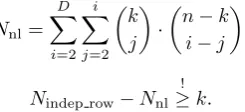
We want to set the parameterkas high as possible in order to reduce the search space for Gray-code enumeration: For every extra variable that can be kept, the search space is halved. As described in the original Crossbred algorithm [11], the maximum of k depends on the Macaulay degree D as well as the number of variables nand the number of equationsmin the originalMQsystem. The number of linearly independent equations that can be extracted from a Macaulay matrix can be computed as the difference of the number of independent rows Nindep rowin the Macaulay matrix and the number of monomials Nnlwhich are
non-linear inx1, . . . , xk. This number must be no less thank; otherwise, there
will not be enough equations in the sub-system to obtain a unique solution. The maximum value ofk forMQ systems withn=m andm= 2n, based on Macaulay degreeD= 3 and 4, can be computed as
Nindep row=
(
m·(n+ 1), whenD= 3,
0 20 40 60 80 100 120 140 160 180 200 0
10 20 30
n
maxim
um
of
k
m=n, D= 3
m=n, D= 4
m= 2n, D= 3
m= 2n, D= 4
Fig. 1: Maximum number of variablesk that can be kept depending onnandm.
Nnl= D
X
i=2 i
X
j=2
k j
·
n−k i−j
,
Nindep row−Nnl !
≥k.
Figure1shows a graph for the number of variables we can keep in relation to the system size forn <200. Clearly, with degree-4 Macaulay matrices one can keep more variables than with degree-3 Macaulay matrices for large enough n. However, for some determined systems, e.g.n= 140, using a degree-4 Macaulay matrix does not allow us to keep more variables than when using a degree-3 matrix. In addition, the gap between the two curves for overdetermined systems becomes narrower as n grows. Therefore, similar to determined systems, the effectiveness of degree-4 matrices is expected to become marginal at which point degree-5 Macaulay matrices are required if one wishes to keep considerably more variables than when using degree-3 matrices.
Note thatkgrows linearly in the beginning of each curve, where the degree of regularity of theMQsystem is smaller than or equal to the Macaulay degree. In this case, a Gr¨obner basis can be extracted directly from the Macaulay matrix, which immediately yields a solution to the system.
4.2 Macaulay Degree
As discussed in [11], since the Macaulay matrix is used to induce cancellation of the monomials where any of the variables x1, x2, . . . , xk has a degree larger
of regularity requirement and that can provide a sufficient number of linearly independent equations for the intended value ofk.
One caveat of choosing the Macaulay degree is that the memory requirement must be smaller than the available system memory. Since both the number of rows and columns of a Macaulay matrix grow considerably when the degree increases, one might have to choose a smaller Macaulay degree and subsequently a smallerkin case the available memory is insufficient.
Our implementation supports both degree-3 and degree-4 Macaulay matrices. Degree-3 Macaulay matrices are useful for small toy examples, while degree-4 Macaulay matrices are sufficient for the largest problem sizes that we target.
4.3 Number of Variables to Fix during External Hybridization
Section4.1gives the formula for computing the maximum value ofkfor a given system. Since the parametern in the formula is the number of variables in the
MQsystem, one can achieve a higherkby fixing somepvariables with external hybridization. In this manner, the number of variables in the system drops by p but the number of equations remains the same. Therefore, the number of variables that can be kept may be higher.
For example, anMQsystem of 148 equations in 74 variables allows to keep k= 21 variables with a degree-4 Macaulay matrix. By fixingp= 4 variables, it becomes a system in 70 variables, which allows to keep one more variable, i.e., k= 22. In this manner, the search space of Gray-code enumeration is split into 24×274−4−22 instead of 1×274−21, which reduces the total number of
itera-tions for Gray-code enumeration by half. On the other hand, 2p sub-systems of
Macaulay matrices need to be computed — so there is a limit on the effectiveness of applying external hybridization.
4.4 Number of Variables to Fix before Exhaustive Search
In addition to fixing variables by external hybridization, one can further fix some variables in the extracted sub-systembeforeentering the exhaustive search stage. By fixing b variables the sub-system beforehand, one can divide the workload evenly into 2b smaller sub-systems which require less resources for applying
ex-haustive search. Clearly, since the main purpose of fixing thesebvariables in the sub-system is to fine-tune the resource requirement, the choice of b should be adjusted based on the hardware architecture and the remaining parameters.
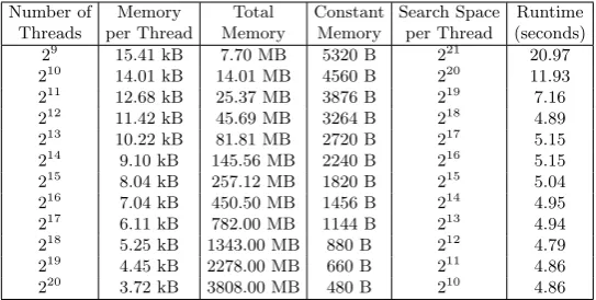
4.5 Number of GPU Threads
Number of Threads
Memory per Thread
Total Memory
Constant Memory
Search Space per Thread
Runtime (seconds)
29 15.41 kB 7.70 MB 5320 B 221 20.97
210 14.01 kB 14.01 MB 4560 B 220 11.93
211 12.68 kB 25.37 MB 3876 B 219 7.16
212 11.42 kB 45.69 MB 3264 B 218 4.89
213 10.22 kB 81.81 MB 2720 B 217 5.15
214 9.10 kB 145.56 MB 2240 B 216 5.15
215 8.04 kB 257.12 MB 1820 B 215 5.04
216 7.04 kB 450.50 MB 1456 B 214 4.95
217 6.11 kB 782.00 MB 1144 B 213 4.94
218 5.25 kB 1343.00 MB 880 B 212 4.79
219 4.45 kB 2278.00 MB 660 B 211 4.86
220 3.72 kB 3808.00 MB 480 B 210 4.86
Table 1: Effect of changing the number of GPU threads.
on a randomly generatedMQsystem of 92 equations in 46 variables with differ-ent numbers of 2t threads. We performed the experiments on a Nvidia Quadro
M1000M GPU using the following settings:
– GPU: Nvidia Quadro M1000M, 4GB off-chip memory, 512 CUDA cores – Macaulay degree:D= 3
– external hybridization:p= 0
– Number of variables to fix before enumeration:b= 0 – Number of variables to keep:k= 16
The results are given in Table1. As expected, the runtime basically remains constant for t ≥12. For t <12, the degree of parallelism is not sufficient and the latencies manifest.
When t = 9, there are 29 = 512 GPU threads deployed, which is exactly the number of CUDA cores available on this particular GPU. In this case, the workload is evenly distributed to all the CUDA cores. Nevertheless, the degree of parallelism is far from enough because executing one single thread per CUDA core is not enough to hide latencies. For example, when the thread loads data from the global memory, which requires hundreds of cycles to access, there is no other thread that can take over the execution resources. Therefore, the CUDA core has no choice but to stall.
Starting from t = 10, there are several threads per CUDA core and some latencies can be hidden. The performance gradually improves untilt= 12, where the degree of parallelism reaches a point where deploying more threads does not improve the ability of the GPU to hide latencies anymore. Therefore, for these experimental settings the threshold where the optimal performance of our implementation can be achieved is 212.
5
Evaluation
We evaluated the performance of our implementation on the Saber clusters [2]. Saber is located at Eindhoven University of Technology and Saber2 at University of Illinois at Chicago. The clusters consist of mostly homogeneous workstations. Out of all the nodes in these two clusters, we used 27 cluster nodes, each equipped with two Nvidia graphics cards. Twelve out of those 27 nodes have two GTX 780 graphics cards while the remaining 15 nodes have two GTX 980 cards. Each node has 32GB RAM and one AMD FX-8350 4GHz processor, which has four physical CPU modules (similar to a physical core in an Intel CPU) shared by eight logical threads (similar to Intel’s hyper threading), 16KB L1 data cache per thread, 2MB L2 cache per module, and 8MB L3 cache shared by the whole CPU. We used CUDA version 7.5 and compiled our implementation with the back-end compiler bundled with CUDA, which is GCC version 4.8.
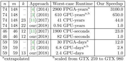
We compare our results to the FES implementations on GPUs from [3] and on FPGAs from [4] and to the Crossbred implementation on CPUs from [11]. Since [3] is using an older GTX 295 graphics card, we scale their results as follows: The GTX 295 graphics card has 480 CUDA cores running at 1242 MHz. Our GTX 980 graphics card has 2048 CUDA cores running at 1278.50 MHz. Therefore, we scale the results of [3] by a factor of 1242
1278· 480
2048 in order to achieve
a rough comparison of the performance. This over-estimates the power of a GTX 295 compared to a GTX 780 and therefore is in favor of [3] in some of the comparisons.
5.1 Overdetermined Systems — Fukuoka MQChallenge
We solved some of theFukuokaMQchallengesusing our implementation. These challenges were created in 2015 in order to help determining appropriate param-eters for public-key cryptographic schemes based onMQsystems. In particular, we chose to target Type-I challenges generated with seed 4 because they consist ofMQsystems innvariables andm= 2nequations overF2.
The experimental results of solving Type-I challenges forn ∈ {55, . . . ,67}
using one single GTX 980 graphics card are given in Table 2. The workflow of the algorithm, i.e., how the search space is split and enumerated, is listed in the 3rd column of the table. For parameters p > 0 and b > 0, external
hybridization and Gray-code enumeration need to be repeated at most 2p and
2b times respectively. The numbers inside the parentheses in the 4th and 5th
n Parameters
(D,p,k,b,t)
Search Space 2p×2b×2n−p−k−b
Extracting Sub-systems
(seconds)
Exhaustive Search (seconds)
Total Runtime (seconds)
Worst-case Runtime (seconds)
55 (4, 0, 19, 0, 14) 1×1×236 387.80 318.25 706.20 706.20
56 (4, 1, 20, 0, 14) 21×1×235 491.60 (1) 169.94 (1) 658.67 1317.34
57 (4, 0, 20, 0, 14) 1×1×237 606.75 650.90 1258.73 1258.73
58 (4, 0, 20, 0, 14) 1×1×238 670.26 1311.97 1982.74 1982.74
59 (4, 0, 20, 0, 14) 1×1×239 741.62 2619.00 3361.77 3361.77
60 (4, 0, 20, 0, 14) 1×1×240 782.12 5211.05 5994.41 5994.41
61 (4, 0, 20, 1, 14) 1×21×240 872.34 5204.18 (1) 6077.13 11280.34
62 (4, 0, 20, 2, 14) 1×22×240 920.24 10485.95 (2) 11407.64 21892.14
63 (4, 4, 21, 0, 14) 24×1×238 9406.21 (11) 14827.94 (11) 24234.15 35250.72
64 (4, 3, 21, 1, 13) 23×21×239 1991.48 (2) 10469.58 (4) 12456.97 49844.24
65 (4, 3, 21, 2, 14) 23×22×239 1046.62 (1) 10517.21 (4) 11565.10 92510.64
66* (4, 1, 21, 5, 13) 21×25×239 16268.10 (2) 133896.93 (51) 151867.70 184295.62
67* (4, 0, 21, 7, 13) 1×27×239 10298.95 198835.78 (74) 209172.34 354231.11
Table 2: Solving overdetermined systems with a single GTX 980 graphics card.
n Parameters
(D,p,k,b,t)
Search Space 2p×2b×2n−p−k−b
Extracting Sub-systems
(seconds)
Total Runtime (seconds)
Worst-case Runtime (GPU-hours)
68 (4, 6, 21, 2, 13) 26×22×239 9799.15 12802.11 214.45
69 (4, 8, 22, 0, 13) 28×1×239 11238.49 56697.70 229.10
70 (4, 7, 22, 2, 13) 27×22×239 14367.71 44223.81 452.65
71 (4, 8, 22, 2, 13) 28×22×239 14392.00 87415.91 947.20
72 (4, 9, 22, 2, 13) 29×22×239 13912.39 144145.58 1867.44
73 (4, 8, 22, 4, 13) 28×24×239 18055.07 159585.32 3700.87
74 (4, 10, 22, 3, 13) 210×23×239 15163.72 118323.38 8236.05
Table 3: Solving overdetermined systems using 27 nodes of the Saber clusters.
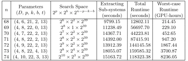
For larger Type-I challenges withn∈ {68, . . . ,74} we used 27 nodes in the Saber and Saber2 clusters by distributing the 2p smallerMQsystems obtained
from external hybridization evenly over the nodes. The results are given in Ta-ble3, which basically has the same format and notation as Table2. In these larger experiments, sub-systems were extracted from degree-4 Macaulay matrices with the CPU because the GPU off-chip memory cannot accommodate the size of the reduced Macaulay matrices. However, these parameters allowed us to pipeline the extraction of sub-systems on the CPU and the exhaustive search stage on the GPU. Therefore, the computation time of the former can be completely hidden except in the first run. Some of the cluster nodes we used have GTX 780 graph-ics cards with only 3GB of off-chip memory while GTX 980 graphgraph-ics cards have 4GB. Therefore, we adjusted the parameters t and b according to the memory size of the GTX 780. Consequently, the 4GB off-chip memory on the GTX 980 was not fully utilized but there was no noticable impact on performance.
Impact of k.The experiments show that despite the number of variables in-creasing by one for each experiment, whenever the maximum value of the pa-rameterkincreases (either with or without external hybridization), the runtime almost stays the same. For example, for the overdetermined MQ systemF68,
n= 68 by keepingk= 21 variables, there are 47 variables left inF68to
n m k Approach Worst-case Runtime Our Speedup
74 148 – [4] (2014) 2900 FPGA-yearsa 3100.0
74 148 – [3] (2010) 610 GPU-yearsa,b 650.0
74 148 23 [11](2017) 41 CPU-years 44.0
74 148 22 our(2018) 0.94 GPU-years 1.0
46 46 12 [11](2017) 1900 CPU-seconds 23.0
46 46 12 our(2018) 82 GPU-seconds 1.0
59 59 – [4] (2014) 30 FPGA-daysa 12.0
59 59 – [3] (2010) 6.8 GPU-daysa,b 2.8
59 59 13 our(2018) 2.4 GPU-days 1.0
aextrapolated bscaled from GTX 259 to GTX 980
Table 4: Worst-case runtime and speedup of our work compared to previous work.
value ofkcan be increased by one (with external hybridization), sok= 22 vari-ables can be kept. Therefore, there are also 47 varivari-ables to enumerate forF69.
Hence, for both systems the total maximum number of iterations that need to be performed during Gray-code enumeration is the same. However, since forF69
linear systems in 22 variables instead of 21 have to be computed, the cost of each iteration of Gray-code enumeration for F69is slightly larger than forF68.
Thus, the worst-case runtime forn= 69 is slightly larger than forn= 68. Comparison. Previous records of solving Type-I challenges were held by the FES and Crossbred algorithms. The FES implementation for FPGAs is able to perform full enumeration over the search space for an MQ system in 64 variables in 956 days [4]. Therefore, it solves aMQ system of 148 equations in 74 variables in at most 274−64·956 days≈2900 FPGA-years. The corresponding
GPU implementation in [3] requires 21 minutes to solve an MQ system with n= 48 variables on a GTX 295 graphics card. Scaling the performance on the GTX 295 to our graphics cards as described before results in 274−48·21 minutes·
1242 1287·
480
2048 ≈610 GPU-years.The original Crossbred implementation for CPUs
requires at most 41 CPU-years to solve the challenge [11] using k = 23. As shown in Table3, our implementation is most efficient withk= 22 and requires at most 8236 GPU-hours, i.e., 0.94 GPU-years. Table 4 shows an overview of the comparison including the respective speedup of our implementation.
Estimated Security for n= 74, m= 2n.As mentioned before, a GTX 980 graphics card consists of 2048 CUDA cores operating at 1278.50 MHz. Based on profiling information, our implementation achieves 37% GPU utilization. There-fore, we estimate the security strength of this particularMQsystem, defined as the number of operations required to solve the system, as
8236.05·2048·1278.50·106·3600·0.37≈264.6.
Thus, anMQsystem withn= 74, m= 2nonly provides about 64-bit security.
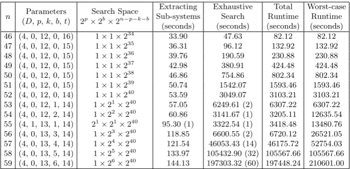
5.2 Determined Systems
n Parameters
(D,p,k,b,t)
Search Space 2p×2b×2n−p−k−b
Extracting Sub-systems
(seconds)
Exhaustive Search (seconds)
Total Runtime (seconds)
Worst-case Runtime (seconds)
46 (4, 0, 12, 0, 16) 1×1×234 33.90 47.63 82.12 82.12
47 (4, 0, 12, 0, 15) 1×1×235 36.31 96.12 132.92 132.92
48 (4, 0, 12, 0, 15) 1×1×236 39.76 190.59 230.88 230.88
49 (4, 0, 12, 0, 15) 1×1×237 42.98 380.91 424.48 424.48
50 (4, 0, 12, 0, 15) 1×1×238 46.86 754.86 802.34 802.34
51 (4, 0, 12, 0, 15) 1×1×239 50.74 1542.07 1593.46 1593.46
52 (4, 0, 12, 0, 14) 1×1×240 53.59 3049.07 3103.21 3103.21
53 (4, 0, 12, 1, 14) 1×21×240 57.05 6249.61 (2) 6307.22 6307.22
54 (4, 0, 12, 2, 14) 1×22×240 60.86 3141.67 (1) 3205.11 12635.54
55 (4, 1, 13, 1, 14) 21×21×240 95.30 (1) 3322.54 (1) 3418.48 13480.76
56 (4, 0, 13, 3, 14) 1×23×240 118.85 6600.55 (2) 6720.12 26521.05
57 (4, 0, 13, 4, 14) 1×24×240 121.54 46053.43 (14) 46175.72 52754.03
58 (4, 0, 13, 5, 14) 1×25×240 133.97 105432.90 (32) 105567.66 105567.66 59 (4, 0, 13, 6, 14) 1×26×240 144.13 197303.32 (60) 197448.24 210601.00
Table 5: Solving determined systems with a single GTX 980 graphics card.
graphics card on a node in the Saber2 cluster. The experimental results are given in Table5, whose format and notation is the same as Table2.
For determined systems, the number of variables that can be kept is much smaller than for overdetermined systems due to that fact that fewer equations are available. However, the linear systems that are enumerated during Gray-code enumeration consist of fewer variables. Therefore, the cost of each iteration is also lower. As Table5shows, solving a determinedMQsystem innvariables is roughly as difficult as solving an overdetermined MQsystem where m0 = 2n0, n0 = n+ 7 ∼ n+ 8. Nevertheless, Figure 1 shows that the gap between the number of variables that can be kept for determined and overdetermined systems gradually becomes larger asngrows. Therefore, this observation only applies to the systems in Table5but not to larger determined systems, e.g.n= 172. Comparison. The extrapolated worst-case runtime of the FES algorithm on FPGAs from [4] is 259−64·956 days≈30 FPGA-days. The corresponding
run-time on GPUs [3] is 259−48·21 minutes·1242 1278·
480
2048 ≈6.8 GPU-days.Our
imple-mentation requires at most 210601 seconds, i.e., about 2.4 GPU-days. Table4 shows the speedup of our implementation. Our speedup over FES forn=m= 59 is significantly lower than forn= 74, m= 148. This shows that the Crossbred al-gorithm is less efficient for smallkand therefore more suitable for larger systems and for overdetermined systems. The authors of the Crossbred-CPU implemen-tation in [11] do not provide performance numbers forn=m= 59. Therefore, we show a comparison forn=m= 46 in Table4.
hidden by pipelining CPU and GPU computations. Extracting a sub-system with these parameters takes 985.86 seconds and each GPU kernel launch takes on average 4338.59 seconds for 240iterations. The worst-case runtime for solving theMQsystem is therefore 4338.59 seconds·2(84−16−40)≈37000 GPU-years.
However, since the probability of obtaining a solution for a determined system is approximately 1− 1
e ≈0.63 [9] and the runtime r for exploring a sub-space
of size 280−16 is r= 4338.59 seconds·2(80−16−40)≈2300 GPU-years (with the
parameters as above), the expected runtime of solving an MQ system where n= 84,m= 80 is only
r·
1−1
e
·
∞ X
i=1
i 1 ei−1 =r·
e
e−1 ≈3600 GPU-years.
Following the calculation in Section5.1, the expected number of operations required for solving such a system on a GPU is therefore
3600·2048·1278.50·106·365·24·3600·0.3706≈276.5,
i.e., these parameters are roughly “76-bit secure” which is very close to the security claimed in [15]. Due to the smallk, the Crossbred algorithm gives only a moderate improvement over the FES algorithm as in [3] with an expected cost of roughly 280·4· e
e−1≈2
82.7 GPU-operations.
However, solving the underlyingMQsystems of this public-key identification scheme using the security parameters of [15] is feasible on average within about one year using 3600 GTX 980 graphics cards at the cost of electricity and about $2 million US dollars for hardware, assuming a price of $550 US dollars per GTX 980 graphics card5. This shows that breaking 80-bit security is within reach at
moderate cost and time using today’s technology and that 128-bit security must be the minimum requirement for multivariate cryptography.
Acknowledgments
We would like to thank Daniel J. Bernstein for granting us access to his Saber GPU clusters at Eindhoven University of Technology and the University of Illi-nois at Chicago. This research was partially supported by the project MOST105-2923-E-001-003-MY3 of the Ministry of Science and Technology, Taiwan.
References
1. Berbain C., Gilbert H., Patarin J.: QUAD: A Practical Stream Cipher with Prov-able Security. In: Vaudenay S. (ed.) Advances in Cryptology — EUROCRYPT 2006. LNCS, vol. 4004, pp. 109–128. Springer (2006)
2. Bernstein D.J.: The Saber Cluster. URL: https://blog.cr.yp.to/20140602-saber.html
5
3. Bouillaguet, C., Chen, H.C., Cheng, C.M., Chou, T., Niederhagen, R., Shamir, A., Yang, B.Y.: Fast Exhaustive Search for Polynomial Systems inF2. In: Mangard, S.,
Standaert, F.X. (eds.) Cryptographic Hardware and Embedded Systems — CHES 2010. LNCS, vol. 6225, pp. 203—218. Springer Berlin Heidelberg (2010)
4. Bouillaguet C., Cheng C.M., Chou T., Niederhagen R., Yang B.Y.: Fast Exhaustive Search for Quadratic Systems inF2on FPGAs. In: Lange T., Lauter K., Lisonˇek P.
(ed.) Selected Areas in Cryptography — SAC 2013. LNCS, vol. 8282, pp. 205–222. Springer (2014)
5. Clough C., Baena J., Ding J., Yang B.Y., Chen M.: Square, a New Multivariate Encryption Scheme. In: Fischlin M. (ed.) Topics in Cryptology — CT-RSA 2009. LNCS, vol. 5473, pp. 252–264. Springer (2009)
6. Ding J., Schmidt D.: Rainbow, a New Multivariable Polynomial Signature Scheme. In: Ioannidis J., Keromytis A., Yung M. (ed.) Applied Cryptography and Network Security — ACNS 2005. LNCS, vol. 3531, pp. 164–175. Springer (2005)
7. Faug`ere J.C.: A new efficient algorithm for computing Gr¨obner bases (F4). Journal
of Pure and Applied Algebra 139, 61–88 (1999)
8. Faug`ere J.C.: A new efficient algorithm for computing Gr¨obner bases without re-duction to zero (F5). In: International Symposium on Symbolic and Algebraic
Computation — ISSAC 2002. pp. 75–83. ACM Press (2002)
9. Fusco G., Bach E.: Phase Transition of Multivariate Polynomial Systems. Mathe-matical Structures in Computer Science 19, 9–23 (2009)
10. J., P.: Hidden Fields Equations (HFE) and Isomorphisms of Polynomials (IP): Two New Families of Asymmetric Algorithms. In: U., M. (ed.) Advances in Cryptology — EUROCRYPT 1996. LNCS, vol. 1070, pp. 33–48. Springer (1996)
11. Joux A., Vitse V.: A Crossbred Algorithm for Solving Boolean Polynomial Systems. IACR Cryptology ePrint Archive (2017),https://eprint.iacr.org/2017/372
12. Kipnis A., Patarin J., Goubin L.: Unbalanced Oil and Vinegar Signature Schemes. In: Stern J. (ed.) Advances in Cryptology — EUROCRYPT 1999. LNCS, vol. 1592, pp. 206–222. Springer (1999)
13. Patarin J., Courtois N., Goubin L.: QUARTZ, 128-Bit Long Digital Signatures. In: Naccache D. (ed.) Topics in Cryptology — CT-RSA 2001. LNCS, vol. 2020, pp. 282–297. Springer (2001)
14. Porras J., Baena J., Ding J.: ZHFE, a New Multivariate Public Key Encryp-tion Scheme. In: Mosca M. (ed.) Post-Quantum Cryptography — PQCrypto 2014. LNCS, vol. 8772, pp. 229–245. Springer, Cham (2014)
15. Sakumoto K., Shirai T., Hiwatari H.: Public-Key Identification Schemes Based on Multivariate Quadratic Polynomials. In: Rogaway P. (ed.) Advances in Cryptology — CRYPTO 2011. LNCS, vol. 6841, pp. 706–723. Springer (2011)
16. Shor, P.W.: Algorithms for Quantum Computation: Discrete Logarithms and Fac-toring. In: Foundations of Computer Science. pp. 124—134. IEEE (1994)
17. Shor, P.W.: Polynomial-Time Algorithms for Prime Factorization and Discrete Logarithms on a Quantum Computer. SIAM Review 41(2), 303—332 (1999) 18. Szepieniec A., Ding J., Preneel B.: Extension Field Cancellation: A New Central
Trapdoor for Multivariate Quadratic Systems. In: Takagi T. (ed.) Post-Quantum Cryptography. LNCS, vol. 9606, pp. 182–196. Springer, Cham (2016)
19. Yang B.-Y., Chen J.-M.: All in the XL Family: Theory and Practice. In: Park C., Chee S. (ed.) Information Security and Cryptology — ICISC 2004. LNCS, vol. 3506, pp. 67–86. Springer (2005)