Real-Valued Function Evaluation
Christina Boura2,1, Ilaria Chillotti2, Nicolas Gama1,2, Dimitar Jetchev1,3, Stanislav Peceny1, Alexander Petric1
1
Inpher, Lausanne, Switzerland and New-York, USA
https://inpher.io
2 Laboratoire de Math´ematiques de Versailles, UVSQ, CNRS, Universit´e
Paris-Saclay, 78035 Versailles, France
3 Ecole Polytechnique F´´ ed´erale de Lausanne, EPFL SB MATHGEOM GR-JET,
Lausanne, Switzerland
Abstract. We propose a novel multi-party computation protocol for evaluating continuous real-valued functions with high numerical preci-sion. Our method is based on approximations with Fourier series and uses at most two rounds of communication during the online phase. For the offline phase, we propose a trusted-dealer and honest-but-curious aided solution, respectively. We apply our algorithm to train a logistic regression classifier via a variant of Newton’s method (known as IRLS) to compute unbalanced classification problems that detect rare events and cannot be solved using previously proposed privacy-preserving op-timization algorithms (e.g., based on piecewise-linear approximations of the sigmoid function). Our protocol is efficient as it can be implemented using standard quadruple-precision floating point arithmetic. We report multiple experiments and provide a demo application that implements our algorithm for training a logistic regression model.
1
Introduction
Privacy-preserving computing allows multiple parties to evaluate a function while keeping the inputs private and revealing only the output of the function and nothing else. Recent advances in multi-party computation (MPC), homomorphic encryption, and differential privacy made these models practical. An example of such computations, with applications in medicine and finance, among others, is the training of supervised models where the input data comes from distinct secret data sources [17], [23], [25], [26] and the evaluation of predictions using these models.
It appears that for a majority of the datasets (e.g., the MNIST database of handwritten digits [15] or the ARCENE dataset [14]), the classification achieves very good accuracy after only a few iterations of the gradient descent using a piecewise-linear approximation of the sigmoid functionsigmo:R→[0,1] defined as
sigmo(x) = 1 1 +e−x,
although the current cost function is still far from the minimum value [25]. Other approximation methods of the sigmoid function have also been proposed in the past. In [29], an approximation with low degree polynomials resulted in a more efficient but less accurate algorithm. Conversely, a higher-degree polyno-mial approximation applied to deep learning algorithms in [24] yielded more ac-curate, but less efficient algorithms (and thus, less suitable for privacy-preserving computing). In parallel, approximation solutions for privacy-preserving methods based on homomorphic encryption [2], [27], [18], [22] and differential privacy [1], [10] have been proposed in the context of both classification algorithms and deep learning.
Nevertheless, accuracy itself is not always a sufficient measure for the quality of the model, especially if, as mentioned in [19, p.423], our goal is to detect a rare event such as a rare disease or a fraudulent financial transaction. If, for example, one out of every one thousand transactions is fraudulent, a na¨ıve model that classifies all transactions as honest achieves 99.9% accuracy; yet this model has no predictive capability. In such cases, measures such as precision, recall and F1-score allow for better estimating the quality of the model. They bound the rates of false positives or negatives relative to only the positive events rather than the whole dataset.
The techniques cited above achieve excellent accuracy for most balanced datasets, but since they rely on a rough approximation of the sigmoid function, they do not converge to the same model and thus, they provide poor scores on datasets with a very low acceptance rate. In this paper, we show how to regain this numerical precision in MPC, and to reach the same score as the plaintext regression. Our MPC approach is mostly based on additive secret shares with precomputed multiplication triplets [4]. This means that the computation is divided in two phases: anoffline phase that can be executed before the data is shared between the players, and anonline phasethat computes the actual result. For the offline phase, we propose a first solution based on atrusted dealer, and then discuss a protocol where the dealer ishonest-but-curious.
1.1 Our contributions
a cost function which is expressed in terms of logarithms of the continuous sig-moid function. This minimum is typically computed via iterative methods such as the gradient descent. For datasets with low acceptance rate, it is important to get much closer to the exact minimum in order to obtain a sufficiently precise model. We thus need to significantly increase the number of iterations (na¨ıve or stochastic gradient descent) or use faster-converging methods (e.g., IRLS [5, §4.3]). The latter require a numerical approximation of the sigmoid that is much better than what was previously achieved in an MPC context, especially when the input data is not normalized or feature-scaled. Different approaches have been considered previously such as approximation by Taylor series around a point (yielding only good approximation locally at that point), or polynomial approximation (by e.g., estimating least squares). Although better than the first one, this method is numerically unstable due to the variation of the size of the coefficients. An alternative method based on approximation by piecewise-linear functions has been considered as well. In MPC, this method performs well when used with garbled circuits instead of secret sharing and masking, but does not provide enough accuracy.
In our case, we approximate the sigmoid using Fourier series, an approach applied for the first time in this context. This method works well as it provides a better uniform approximation assuming that the function is sufficiently smooth (as is the case with the sigmoid). In particular, we virtually re-scale and extend the sigmoid to a periodic function that we approximate with a trigonometric polynomial which we then evaluate in a stable privacy-preserving manner. To approximate a generic function with trigonometric polynomials that can be eval-uated in MPC, one either use the Fourier series of a smooth periodic extension or finds directly the closest trigonometric polynomial by the method of least squares for the distance on the half-period. The first approach yields a super-algebraic convergence at best, whereas the second converges exponentially fast. On the other hand, the first one is numerically stable whereas the second one is not (under the standard Fourier basis). In the case of the sigmoid, we show that one can achieve both properties at the same time.
Significant reduction in communication time. In this paper, we follow the same approach as in [25] and define dedicated triplets for high-level instructions, such as large matrix multiplications, a system resolution, or an oblivious evaluation of the sigmoid. This approach is less generic than masking low-level instructions as in SPDZ, but it allows to reduce the communication and memory requirements by large factors. Masks and operations are aware of the type of vector or matrix dimensions and benefit from the vectorial nature of the high-level operations. For example, multiplying two matrices requires a single round of communication instead of up toO(n3) for coefficient-wise approaches, depending on the batching quality of the compiler. Furthermore, masking is defined per immutable variable rather than per elementary operation, so a constant matrix is masked only once during the whole algorithm. Combined with non-trivial local operations, these triplets can be used to achieve much more than just ring additions or multiplica-tions. In a nutshell, the amount of communications is reduced as a consequence of reusing the same masks, and the number of communication rounds is re-duced as a consequence of masking directly matrices and other large structures. Therefore, the total communication time becomes negligible compared to the computing cost.
New protocol for the honest but curious offline phase extendable to n players. We introduce a new protocol for executing the offline phase in the honest-but-curious model that is easily extendable to a generic number nof players while remaining efficient. To achieve this, we use a broadcast channel instead of peer-to-peer communication which avoids a quadratic explosion in the number of communications. This is an important contribution, as none of the previous protocols forn > 3 players in this model are efficient. In [17], for instance, the authors propose a very efficient algorithm in the trusted dealer model; yet the execution time of the oblivious transfer protocol is quite slow.
2
Notation and Preliminaries
Assume thatP1, . . . , Pnare distinct computing parties (players). We recall some basic concepts from multi-party computation that will be needed for this paper.
2.1 Secret sharing and masking
Let (G,•) be a group and letx∈Gbe a group element.
Asecret shareofx, denoted byJxK•(by a slight abuse of notation), is a tuple
(x1, . . . , xn)∈ Gn such that x=x1• · · · •xn. If (G,+) is abelian, we call the
secret sharesx1, . . . , xnadditive secret shares. A secret sharing scheme is compu-tationally secure if for any two elementsx, y∈G, strict sub-tuples of sharesJxK•
orJyK•are indistinguishable. IfGadmits a uniform distribution, an
information-theoretic secure secret sharing scheme consists of drawingx1, . . . , xn−1uniformly at random and choosingxn =x−n−11• · · · •x
−1
A closely related notion is the one of group masking. Given a subset X of
G, the goal of masking X is to find a distribution D over G such that the distributions ofx•Dforx∈ X are all indistinguishable. Indeed, such distribution can be used to create a secret share: one can sampleλ← D, and giveλ−1 to a player and x•λto the other. Masking can also be used to evaluate non-linear operations in clear over masked data, as soon as the result can be privately unmasked via homomorphisms (as in, e.g., the Beaver’s triplet multiplication technique [4]).
2.2 Arithmetic with secret shares via masking
Computing secret shares for a sumx+y (or a linear combination if (G,+) has a module structure) can be done non-interactively by each player by adding the corresponding shares of x and y. Computing secret shares for a product is more challenging. One way to do that is to use an idea of Beaver based on precomputed and secret shared multiplicative triplets. From a general point of view, let (G1,+), (G2,+) and (G3,+) be three abelian groups and letπ:G1×
G2→G3be a bilinear map.
Given additive secret shares JxK+ and JyK+ for two elements x ∈ G1 and y ∈ G2, we would like to compute secret shares for the element π(x, y) ∈G3. With Beaver’s method, the players must employ precomputed single-use random triplets (JλK+,JµK+,Jπ(λ, µ)K+) for λ∈G1 and µ∈ G2, and then use them to
mask and reveal a = x+λ and b = y+µ. The players then compute secret shares forπ(x, y) as follows:
– Player 1 computesz1=π(a, b)−π(a, µ1)−π(λ1, b) + (π(λ, µ))1;
– Playeri(fori= 2, . . . , n) computes zi=−π(a, µi)−π(λi, b) + (π(λ, µ))i. The computed z1, . . . , zn are the additive shares of π(x, y). A given λ can be used to mask only one variable, so one triplet must be precomputed for each multiplication during the offline phase (i.e. before the data is made available to the players). Instantiated with the appropriate groups, this abstract scheme allows to evaluate a product in a ring, but also a vectors dot product, a matrix-vector product, or a matrix-matrix product.
2.3 MPC evaluation of real-valued continuous functions
For various applications (e.g., logistic regression in Section 6), we need to com-pute continuous real-valued functions over secret shared data. For non-linear functions (e.g. exponential, log, power, cos, sin, sigmoid, etc.), different methods are proposed in the literature.
The second approach is to replace the function with an approximation that is easier to compute: for instance, [25] uses garbled circuits to evaluate fixed point comparisons and absolute values; it then replaces the sigmoid function in the logistic regression with a piecewise-linear function. Otherwise, [24] approximates the sigmoid with a polynomial of fixed degree and evaluates that polynomial with the Horner method, thus requiring a number of rounds of communications proportional to the degree.
Another method that is close to how SPDZ [13] computes inverses in a finite field, is based on polynomial evaluation via multiplicative masking: using a pre-computed triplet of the form (JλK+,Jλ
−1
K+, . . . ,Jλ −p
K+), players can evaluate
P(x) = Pp
i=0apxp by revealing u=xλ and outputting the linear combination
Pp
i=0aiuiJλ −i
K+.
Multiplicative masking, however, involves some leakage: in finite fields, it reveals whetherxis null. The situation gets even worse in finite rings where the multiplicative orbit ofxis disclosed (for instance, the rank would be revealed in a ring of matrices), and overR, the order of magnitude ofxwould be revealed. For real-valued polynomials, the leakage could be mitigated by translating and rescaling the variablexso that it falls in the range [1,2). Yet, in general, the coefficients of the polynomials that approximate the translated function explode, thus causing serious numerical issues.
2.4 Full threshold honest-but-curious protocol
3
Statistical Masking and Secret Share Reduction
In this section, we present in this section our masking technique for fixed-point arithmetic and provide an algorithm for the MPC evaluation of real-valued con-tinuous functions. In particular, we show that to achieve p bits of numerical precision in MPC, it suffices to havep+ 2τ-bit floating points whereτ is a fixed security parameter.
The secret shares we consider are real numbers. We would like to mask these shares using floating point numbers. Yet, as there is no uniform distribution on R, no additive masking distribution over reals can perfectly hide the arbi-trary inputs. In the case when the secret shares belong to some known range of numerical precision, it is possible to carefully choose a masking distribution, de-pending on the precision range, so that the masked value computationally leaks no information about the input. A distribution with sufficiently large standard deviation could do the job: for the rest of the paper, we refer to this type of masking as “statistical masking”. In practice, we choose a normal distribution with standard deviationσ= 240.
On the other hand, by using such masking, we observe that the sizes of the secret shares increase every time we evaluate the multiplication via Beaver’s technique (Section 2.2). In Section 3.3, we address this problem by introducing a technique that allows to reduce the secret share sizes by discarding the most significant bits of each secret share (using the fact that the sum of the secret shares is still much smaller than their size).
3.1 Floating point, fixed point and interval precision
Suppose that B is an integer and that pis a non-negative integer (the number of bits). The class of fixed-point numbers of exponentBand numerical precision
pis:
C(B, p) ={x∈2B−p·Z,|x| ≤2B}.
Each classC(B, p) is finite, and contains 2p+1+1 numbers. They could be rescaled and stored as (p+ 2)-bit integers. Alternatively, the number x ∈ C(B, p) can also be represented by the floating point value x, provided that the floating point representation has at least pbits of mantissa. In this case, addition and multiplication of numbers across classes of the same numerical precision are natively mapped to floating-point arithmetic. The main arithmetic operations on these classes are:
– Lossless Addition:C(B1, p1)×C(B2, p2)→ C(B, p) whereB=max(B1, B2)+
1 andp=B−min(B1−p1, B2−p2);
– Lossless Multiplication:C(B1, p1)× C(B2, p2)→ C(B, p) whereB =B1+
B2 andp=p1+p2;
– Rounding: C(B1, p1) → C(B, p), that maps x to its nearest element in
Lossless operations require p to increase exponentially in the multiplication depth, whereas fixed precision operations maintain p constant by applying a final rounding. Finally, note that the exponent B should be incremented to store the result of an addition, yet,B is a user-defined parameter in fixed point arithmetic. If the user forcibly chooses to keepBunchanged, any result|x|>2B will not be representable in the output domain (we refer to this type of overflow asplaintext overflow).
3.2 Floating point representation
Given a security parameter τ, we say that a set S is a τ-secure masking set for a class C(B, p) if the following distinguishability game cannot be won with advantage ≥ 2−τ: the adversary chooses two plaintexts m
0, m1 in C(B, p), a challenger picks b ∈ {0,1} and α ∈ S uniformly at random, and sends c =
mb+αto the adversary. The adversary has to guessb. Note that increasing such distinguishing advantage from 2−τ to ≈ 1/2 would require to give at least 2τ samples to the attacker, soτ = 40 is sufficient in practice.
Proposition 1. The class C(B, p, τ) ={α∈2B−p
Z,|α| ≤2B+τ} is a τ-secure masking set forC(B, p)
Proof. If a, b ∈ C(B, p) and U is the uniform distribution on C(B, p, τ), the statistical distance betweena+U andb+U is (b−a)·2p−B/#C(B, p, τ)≤2−τ. This distance upper-bounds any computational advantage. ut Again, the classC(B, p, τ) =C(B+τ, p+τ) fits in floating point numbers of
p+τ-bits of mantissa, so they can be used to securely mask fixed point numbers with numerical precision p. By extension, all additive shares forC(B, p) will be taken inC(B, p, τ).
We now analyze what happens if we use Beaver’s protocol to multiply two plaintexts x∈ C(B1, p) and y ∈ C(B2, p). The masked valuesx+λ and y+µ are bounded by 2B1+τ and 2B2+τ respectively. Since the maskλis also bounded
by 2B1+τ, andµ by 2B2+τ, the computed secret shares of x·y will be bounded
by 2B1+B2+2τ, So the lossless multiplication sends C(B
1, p, τ)× C(B2, p, τ) →
C(B,2p,2τ) whereB=B1+B2instead ofC(B, p, τ). Reducingpis just a matter of rounding, and it is done automatically by the floating point representation. However, we still need a method to reduce τ, so that the output secret shares are bounded by 2B+τ.
3.3 Secret share reduction algorithm
The algorithm we propose depends on two auxiliary parameters: thecutoff, de-fined as η = B+τ so that 2η is the desired bound in absolute value, and an auxiliary parameterM = 2κ larger than the number of players.
bits of the share beyond the cutoff position (say MSB(zi) = bzi/2ηe) do not contain any information on the data, and are all safe to reveal. We also know that the MSB of the sum of the shares (i.e. MSB of the data) is null, so the sum of the MSB of the shares is very small. The share reduction algorithm simply computes this sum, and redistributes it evenly among the players. Since the sum is guaranteed to be small, the computation is done modulo M rather than on large integers. More precisely, using the cutoff parameter η, for i = 1, . . . , n, player i writes his secret sharezi of z as zi =ui+ 2ηvi, with vi ∈Z andui ∈ [−2η−1,2η−1). Then, he broadcastsv
i modM, so that each player computes the sum. The individual shares can optionally be re-randomized using a precomputed shareJνK+, withν = 0 modM. Since w=P
vi’s is guaranteed to be between −M/2 andM/2, it can be recovered from its representation modM. Thus, each player locally updates its share as ui+ 2ηw/n, which have by construction the same sum as the original shares, but are bounded by 2η. This construction is summarized in Algorithm 3 in Appendix B.
4
Fourier Approximation
Fourier theory allows us to approximate certain periodic functions with trigono-metric polynomials. The goal of this section is two-fold: to show how to evaluate trigonometric polynomials in MPC and, at the same time, to review and show extensions of some approximation results to non-periodic functions.
4.1 Evaluation of trigonometric polynomials
Recall that a complex trigonometric polynomial is a finite sum of the form
t(x) =PP
m=−Pcmeimx, where cm ∈Cis equal toam+ibm, witham, bm ∈R. Each trigonometric polynomial is a periodic function with period 2π. Ifc−m=cm for allm∈Z, thentis real-valued, and corresponds to the more familiar cosine decomposition t(x) = a0+PNm=1amcos(mx) +bmsin(mx). Here, we describe how to evaluate trigonometric polynomials in an MPC context, and explain why it is better than regular polynomials.
We suppose that, for all m, the coefficients am and bm of t are publicly accessible and they are 0≤am, bm≤1. As t is 2πperiodic, we can evaluate it on inputs modulo 2π. Remark that asR mod 2πadmits a uniform distribution, we can use a uniform masking: this method completely fixes the leakage issues that were related to the evaluation of classical polynomials via multiplicative masking. On the other hand, the output of the evaluation is still in R: in this case we continue using the statistical masking described in previous sections. The inputs are secretly shared and additively masked: for sake of clarity, to distinguish the classical addition over reals from the addition modulo 2π, we temporarily denote this latter by ⊕. In the same way, we denote the additive secret shares with respect to the addition modulo 2πbyJ·K⊕. Then, the transition
Then, a way to evaluatet on a secret shared inputJxK+= (x1, . . . , xn) is to convertJxK+ toJxK⊕ and additively mask it with a shared masking JλK⊕, then
revealx⊕λand rewrite our targetJeimx
K+ase
im(x⊕λ)·
Je
im(−λ)
K+. Indeed, since x⊕λis revealed, the coefficienteim(x⊕λ)can be computed in clear. Overall, the whole trigonometric polynomialtcan be evaluated in a single round of commu-nication, given a precomputed triplet such as (JλK⊕,Je
−iλ
K+, . . . ,Je −iλP
K+) and
thanks to the fact thatx⊕λhas been revealed.
Also, we notice that to work with complex numbers of absolute value 1 makes the method numerically stable, compared to power functions in regular polyno-mials. It is for this reason that the evaluation of trigonometric polynomials is a better solution in our context.
4.2 Approximating non-periodic functions
If one is interested in uniformly approximating (with trigonometric polynomi-als on a given interval, e.g. [−π/2, π/2]) a non-periodic functionf, one cannot simply use the Fourier coefficients. Indeed, even if the function is analytic, its Fourier series need not converge uniformly near the end-points due to Gibbs phenomenon.
Approximations viaC∞-extensions. One way to remedy this problem is to look for a periodic extension of the function to a larger interval and look at the convergence properties of the Fourier series for that extension. To obtain expo-nential convergence, the extension needs to be analytic too, a condition that can rarely be guaranteed. In other words, the classical Whitney extension theorem [28] will rarely yield an analytic extension that is periodic at the same time. A constructive approach for extending differentiable functions is given by Hestenes [20] and Fefferman [16] in a greater generality. The best one can hope for is to extend the function to aC∞-function (which is not analytic). As explained in [8], [9], such an extension yields a super-algebraic approximation at best that is not exponential.
Approximating the sigmoid function. We now restrict to the case of the sigmoid function over the interval [−B/2, B/2] for some B > 0. We can rescale the variable to approximateg(x) =sigmo(Bx/π) over [−π/2, π/2]. If we extendgby anti-periodicity (odd-even) to the interval [π/2,3π/2] with the mirror condition
g(x) =g(π−x), we obtain a continuous 2π-periodic piecewise C1 function. By Dirichlet’s global theorem, the Fourier serie ofg converges uniformly overR, so for allε >0, there exists a degreeNand a trigonometric polynomialgNsuch that kgN−gk∞≤. To computesigmo(t) over secret sharedt, we first apply the affine
change of variable (which is easy to evaluate in MPC), to get the corresponding
x∈[−π/2, π/2], and then we evaluate the trigonometric polynomialgN(x) using a Fourier triplet. This method is sufficient to get 24 bits of precision with a polynomial of only 10 terms, however asymptotically, the convergence rate is only in Θ(n−2) due to discontinuities in the derivative of g. In other words, approximating g with λ bits of precision requires to evaluate a trigonometric polynomial of degree 2λ/2. Luckily, in the special case of the sigmoid function, we can make this degree polynomial by explicitly constructing a 2π-periodic analytic function that is exponentially close to the rescaled sigmoid on the whole interval [−π, π] (not the half interval). Besides, the geometric decay of the coefficients of the trigonometric polynomial ensures perfect numerical stability. The following theorem, whose proof can be found in Appendix D summarizes this construction.
Theorem 1. Lethα(x) = 1/(1 +e−αx)−x/2πforx∈(−π, π). For everyε >0,
there existsα=O(log(1/ε))such thathα is at uniform distanceε/2from a2π -periodic analytic function g. There exists N =O(log2(1/ε))such that the Nth term of the Fourier series ofg is at distanceε/2 ofg, and thus, at distance≤ε
fromhα.
5
Honest but Curious Model
In the previous sections, we defined the shares of multiplication, power and Fourier triplets, but did not explain how to generate them. Of course, a single trusted dealer approved by all players (TD model) could generate and distribute all the necessary shares to the players. Since the trusted dealer knows all the masks, and thus all the data, the TD model is only legitimate for few computa-tion outsourcing scenarios.
We now explain how to generate the same triplets efficiently in the more tra-ditionalhonest-but-curious (HBC) model. To do so, we keep an external entity, called again the dealer, who participates in an interactive protocol to generate the triplets, but sees only masked information. Since the triplets in both the HBC and TD models are similar, the online phase is unchanged. Notice that in this HBC model, even if the dealer does not have access to the secret shares, he still has more power than the players. In fact, if one of the players wants to gain information on the secret data, he has to collude with all other players, whereas the dealer would need to collaborate with just one of them.
Algorithm 1Honest but curious triplets generation for a trigonometric poly Output: Shares (JλK,Jeim1λ
K+, . . . ,Je
imNλ
K+).
1: Each playerPigeneratesλi, ai (uniformly modulo 2π) 2: Each playerPibroadcastsai to all other players. 3: Each player computesa=a1+· · ·+an mod 2π. 4: Each playerPisends to the dealerλi+ai mod 2π.
5: The dealer computesλ+a mod 2πandw(1)=eim1(λ+a), . . . , w(N)=eimN(λ+a) 6: The dealer createsJw(1)K+, . . . ,Jw
(N)
K+and sendsw
(1) i , . . . , w
(N)
i to playerPi. 7: Each playerPimultiplies eachw(ij)bye
−imjato get (eimjλ)
i, for allj∈[1, N].
assume that an additional private broadcast channel (a channel to which the dealer has no access) exists between all the players (Figure 5 in Appendix E). Afterwards, the online phase only requires a public broadcast channel between the players (Figure 6 in Appendix E). In practice, because of the underlying encryption, private channels (e.g., SSL connections) have a lower throughput (generally ≈20MB/s) than public channels (plain TCP connections, generally from 100 to 1000MB/s between cloud instances).
The majority of HBC protocols proposed in the literature present a scenario with only 2 players. In [11] and [3], the authors describe efficient HBC protocols that can be used to perform a fast MPC multiplication in a model with three players. The two schemes assume that the parties follow correctly the protocol and that two players do not collude. The scheme proposed in [11] is very complex to scale for more than three parties, while the protocol in [3] can be extended to a generic number of players, but requires a quadratic number of private channels (one for every pair of players). We propose a different protocol for generating the multiplicative triplets in the HBC scenario, that is efficient for any arbitrary number n of players. In our scheme, the dealer evaluates the non-linear parts in the triplet generation, over the masked data produced by the players, then he distributes the masked shares. The mask is common to all players, and it is produced thanks to the private broadcast channel that they share. Finally, each player produces his triplet by unmasking the precomputed data received from the dealer.
In Appendix E, we present in detail two algorithms: one for the generation of multiplicative Beaver’s triplets (Algorithm 4) and the other for the generation of the triplets used in the computation of the power function (Algorithm 5), both in the honest-but-curious scenario. Following the same ideas, Algorithm 1 describes our triplets generation for the evaluation of a trigonometric polynomial in the HBC scenario.
6
Application to Logistic Regression
In a classification problem one is given a data set, also called a training set, that we will represent here by a matrix X ∈ MN,k(R), and a training vector
coordinateyi of the vectory corresponds to the class (0 or 1) to which thei-th element of the data set belongs to. Formally, the goal is to determine a function
hθ:Rk→ {0,1}that takes as input a vectorx, containingkfeatures, and which outputshθ(x) predicting reasonably welly, the corresponding output value.
In logistic regression typically one uses hypothesis functions hθ : Rk+1 → [0,1] of the formhθ(x) =sigmo(θTx), where θTx=Pki=0θixi∈Randx0= 1. The vector θ, also called model, is the parameter that needs to be determined. For this, a convexcost function Cx,y(θ) measuring the quality of the model at a data point (x, y) is defined as
Cx,y(θ) =−yloghθ(x)−(1−y) log(1−hθ(x)). The cost for the whole dataset is thus computed as PN
i=1Cxi,yi(θ). The overall goal is to determine a model θ whose cost function is as close to 0 as possible. A common method to achieve this is the so called gradient descent which consists of constantly updating the modelθas
θ:=θ−α∇Cx,y(θ),
where ∇Cx,y(θ) is the gradient of the cost function and α > 0 is a constant called thelearning rate. Choosing the optimalαdepends largely on the quality of the dataset: ifαis too large, the method may diverge, and ifαis too small, a very large number of iterations are needed to reach the minimum. Unfortu-nately, tuning this parameter requires either to reveal information on the data, or to have access to a public fake training set, which is not always feasible in private MPC computations. This step is often silently ignored in the literature. Similarly, preprocessing techniques such as feature scaling, or orthogonalization techniques can improve the dataset, and allow to increase the learning rate sig-nificantly. But again, these techniques cannot easily be implemented when the input data is shared, and when correlation information should remain private. In this work, we choose to implement the IRLS method [5,§4.3], which does not require feature scaling, works with learning rate 1, and converges in much less iterations, provided that we have enough floating point precision. In this case, the model is updated as:
θ:=θ−H(θ)−1· ∇Cx,y(θ), whereH(θ) is the Hessian matrix.
6.1 Implementation and Experimental Results
CPU, 128-bit floating point arithmetic is emulated using GCC’s quadmath li-brary, however additional speed-ups could be achieved on more recent hardware that natively supports these operations (eg. IBM’s next POWER9 processor). In our proof of concept, our main focus was to improve the running time, the floating point precision, and the communication complexity of the online phase, so we implemented the offline phase only for the trusted dealer scenario, leaving the honest but curious dealer variant as a future work.
Algorithm 2Model training:Train(X,y)
Input: A datasetX∈ MN,k(R) and a training vectory∈ {0,1}N Output: The modelθ∈Rk that minimizesCostX,y(θ)
1: Precompute Prodsi=XiTXifori∈[0, N−1] 2: θ←[0, . . . ,0]∈Rk
3: foriter = 1 to IRLS ITERSdo . In practice IRLS ITERS = 8 4: a←X·θ
5: p←[sigmo(a0), . . . ,sigmo(aN−1)]
6: pmp←[p0(1−p0), . . . , pN−1(1−pN−1)]
7: grad←XT(p−y) 8: H ←pmp·Prods 9: θ=θ−H−1·grad 10: end for
11: returnθ
Model-training algorithm with the IRLS method. The algorithm is explained over the plaintext. In the MPC instantiation, each player gets a secret share for each variables. Every product is evaluated using the bilinear formula of Section 2, and the sigmoid using the Fourier method of Section 4.
We implemented the logistic regression model training described in Algo-rithm 2. Each iteration of the main loop evaluates the gradient (grad) and the Hessian (H) of the cost function at the current positionθ, and solves the Hes-sian system (line 7) to find the next position. Most of the computation steps are bilinear on large matrices or vectors, and each of them is evaluated via a Beaver triplet in a single round of communication. In step 5 the sigmoid functions are approximated (in parallel) by an odd trigonometric polynomial of degree 23, which provides 20 bits of precision on the whole interval. We therefore use a vector of Fourier triplets, as described in Section 4. The Hessian system (step 9) is masked by two (uniformly random) orthonormal matrices on the left and the right, and revealed, so the resolution can be done in plaintext. Although this method reveals the norm of the gradient (which is predictable anyway), it hides its direction entirely, which is enough to ensure that the final model remains pri-vate. Finally, since the input data is not necessarily feature-scaled, it is essential to start from the zero position (step 2) and not a random position, because the first one is guaranteed to be in the IRLS convergence domain.
instructions on immutable variables (which are read-only once they are affected). More importantly, the compiler associates a single additive maskλU to each of these immutable variablesU. This solves two important problems that we saw in the previous sections: first, the masking information for huge matrices that are re-used throughout the algorithm are transmitted only once during the whole protocol (this optimization already appears in [25], and in our case, it has a huge impact for the constant input matrix, and their precomputed products, which are re-used in all IRLS iterations). It also mitigates the attack that would retrieve information by averaging its masked distribution, because an attacker never gets two samples of the same distribution. This justifies the choice of 40 bits of security for masking.
During the offline phase, the trusted dealer generates one random mask value for each immutable variable, and secret shares these masks. For all matrix-vector or matrix-matrix products between any two immutable variablesU andV (com-ing from lines 1, 4, 6, 7 and 8 of Alg.2), the trusted dealer also generates a specific multiplication triplet using the masksλU ofU andλV ofV. More pre-cisely, he generates and distributes additive shares forλU·λV as well as integer vectors/matrices of the same dimensions as the product for the share-reduction phase. These integer coefficients are taken modulo 256 for efficiency reasons.
6.2 Results
We implemented all the described algorithms and we tested our code for two and three parties, using cloud instances on both the AWS and the Azure platforms, having Xeon E5-2666 v3 processors. In our application each instance commu-nicates via its public IP address. Furthermore, we use the zeroMQ library to handle low-level communications between the players (peer-to-peer, broadcast, central nodes etc...).
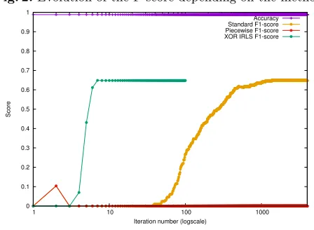
Finally, when the input data is guaranteed to be feature-scaled, we can im-prove the whole time, memory and communication complexities by about 30% by performing 3 classical gradient descent iterations followed by 5 IRLS iter-ations instead of 8 IRLS iteriter-ations. We tested this optimization for both the plaintext and the MPC version and in Appendix A, we show the evolution of the cost function, during the logistic regression, and of the F-score (Figure 1 and 2), depending on the method used.
We have tested our platform on datasets that were provided by the banking industry. For privacy reasons, these datasets cannot be revealed. However, the behaviour described in this paper can be reproduced by generating random data sets, for instance, with Gaussian distribution, setting the acceptance threshold to 0.5%, and adding some noise by randomly swapping a few labels. Readers interested in testing the platform should contact the authors.
Open problems. A first important open question is the indistinguishability of
the distributions after our noise reduction algorithm. On a more fundamental level, one would like to find a method of masking using the basis of half-range Chebyshev polynomials defined in the appendix as opposed to the standard Fourier basis. Such a method, together with the exponential approximation, would allow us to evaluate (in MPC) any function inL2([−1,1]).
Acknowledgements
We thank Hunter Brooks, Daniel Kressner and Marco Picasso for useful conver-sations on data-independent iterative optimization algorithms. We are grateful to Jordan Brandt, Alexandre Duc and Morten Dahl for various useful discussions regarding multi-party computations and privacy-preserving machine learning.
References
1. M. Abadi, A. Chu, I. Goodfellow, H. Brendan McMahan, I. Mironov, K. Talwar, and L. Zhang. Deep learning with differential privacy. CoRR, abs/1607.00133, 2016.
2. Y. Aono, T. Hayashi, L. Trieu Phong, and L. Wang. Privacy-preserving logis-tic regression with distributed data sources via homomorphic encryption. IEICE Transactions, 99-D(8):2079–2089, 2016.
3. T. Araki, J. Furukawa, Y. Lindell, A. Nof, and K. Ohara. High-throughput semi-honest secure three-party computation with an semi-honest majority. InProceedings of the 2016 ACM SIGSAC Conference on Computer and Communications Security, Vienna, Austria, October 24-28, 2016, pages 805–817, 2016.
4. D. Beaver. Efficient Multiparty Protocols Using Circuit Randomization. In
CRYPTO ’91, volume 576 ofLecture Notes in Computer Science, pages 420–432. Springer, 1992.
6. D. Bogdanov, S. Laur, and J. Willemson. Sharemind: A framework for fast privacy-preserving computations. InESORICS 2008, pages 192–206. Springer, 2008. 7. J. Boyd. A comparison of numerical algorithms for Fourier extension of the first,
second, and third kinds. J. Comput. Phys., 178(1):118–160, May 2002.
8. J. Boyd. Fourier embedded domain methods: Extending a function defined on an irregular region to a rectangle so that the extension is spatially periodic andc∞.
Appl. Math. Comput., 161(2):591–597, February 2005.
9. J. Boyd. Asymptotic fourier coefficients for aCinfinity bell (smoothed-”top-hat”) & the fourier extension problem. J. Sci. Comput., 29(1):1–24, 2006.
10. K. Chaudhuri and C. Monteleoni. Privacy-preserving logistic regression. In Daphne Koller, Dale Schuurmans, Yoshua Bengio, and L´eon Bottou, editors,Advances in Neural Information Processing Systems 21, Proceedings of the Twenty-Second An-nual Conference on Neural Information Processing Systems, Vancouver, British Columbia, Canada, December 8-11, 2008, pages 289–296. Curran Associates, Inc., 2008.
11. R. Cramer, I. Damg˚ard, and J. B. Nielsen. Secure Multiparty Computation and Secret Sharing. Cambridge University Press, 2015.
12. I. Damg˚ard, V. Pastro, N. Smart, and S. Zakarias. Multiparty computation from somewhat homomorphic encryption. In Reihaneh Safavi-Naini and Ran Canetti, editors,Advances in Cryptology - CRYPTO 2012 - 32nd Annual Cryptology Con-ference, Santa Barbara, CA, USA, August 19-23, 2012. Proceedings, volume 7417 ofLecture Notes in Computer Science, pages 643–662. Springer, 2012.
13. I. Damg˚ard, V. Pastro, N. P. Smart, and S. Zakarias. SPDZ Software.
https://www.cs.bris.ac.uk/Research/CryptographySecurity/SPDZ/.
14. Dataset. Arcene Data Set.https://archive.ics.uci.edu/ml/datasets/Arcene. 15. Dataset. MNIST Database. http://yann.lecun.com/exdb/mnist/.
16. C. Fefferman. Interpolation and extrapolation of smooth functions by linear oper-ators. Rev. Mat. Iberoamericana, 21(1):313–348, 2005.
17. A. Gasc´on, P. Schoppmann, B. Balle, M. Raykova, J. Doerner, S. Zahur, and D. Evans. Privacy-preserving distributed linear regression on high-dimensional data. Proceedings on Privacy Enhancing Technologies, 4:248–267, 2017.
18. R. Gilad-Bachrach, N. Dowlin, K. Laine, K. E. Lauter, M. Naehrig, and J. Werns-ing. Cryptonets: Applying neural networks to encrypted data with high through-put and accuracy. InProceedings of the 33nd International Conference on Machine Learning, ICML 2016, New York City, NY, USA, June 19-24, 2016, pages 201–210, 2016.
19. I. Goodfellow, Y. Bengio, and A. Courville. Deep Learning. MIT Press, 2016.
http://www.deeplearningbook.org.
20. M. R. Hestenes. Extension of the range of a differentiable function. Duke Math. J., 8:183–192, 1941.
21. D. Huybrechs. On the fourier extension of nonperiodic functions. SIAM J. Nu-merical Analysis, 47(6):4326–4355, 2010.
22. A. J¨aschke and F. Armknecht. Accelerating homomorphic computations on ra-tional numbers. In ACNS 2016, volume 9696 ofLNCS, pages 405–423. Springer, 2016.
23. Y. Lindell and B. Pinkas. Privacy preserving data mining. InAdvances in Cryp-tology - CRYPTO 2000, 20th Annual International CrypCryp-tology Conference, Santa Barbara, California, USA, August 20-24, 2000, Proceedings, pages 36–54, 2000. 24. R. Livni, S. Shalev-Shwartz, and O. Shamir. On the computational efficiency of
Neil D. Lawrence, and Kilian Q. Weinberger, editors,Advances in Neural Informa-tion Processing Systems 27: Annual Conference on Neural InformaInforma-tion Processing Systems 2014, December 8-13 2014, Montreal, Quebec, Canada, pages 855–863, 2014.
25. P. Mohassel and Y. Zhang. SecureML: A system for scalable privacy-preserving machine learning. In 2017 IEEE Symposium on Security and Privacy, SP 2017, San Jose, CA, USA, May 22-26, 2017, pages 19–38. IEEE Computer Society, 2017. 26. V. Nikolaenko, U. Weinsberg, S. Ioannidis, M. Joye, D. Boneh, and N. Taft. Privacy-preserving ridge regression on hundreds of millions of records. In 2013 IEEE Symposium on Security and Privacy, SP 2013, Berkeley, CA, USA, May 19-22, 2013, pages 334–348. IEEE Computer Society, 2013.
27. L. Trieu Phong, Y. Aono, T. Hayashi, L. Wang, and S. Moriai. Privacy-preserving deep learning: Revisited and enhanced. In Lynn Batten, Dong Seong Kim, Xuyun Zhang, and Gang Li, editors,Applications and Techniques in Information Security -8th International Conference, ATIS 2017, Auckland, New Zealand, July 6-7, 2017, Proceedings, volume 719 ofCommunications in Computer and Information Science, pages 100–110. Springer, 2017.
28. H. Whitney. Analytic extensions of differentiable functions defined in closed sets.
Trans. Amer. Math. Soc., 36(1):63–89, 1934.
A
Timings for
n
= 3 players
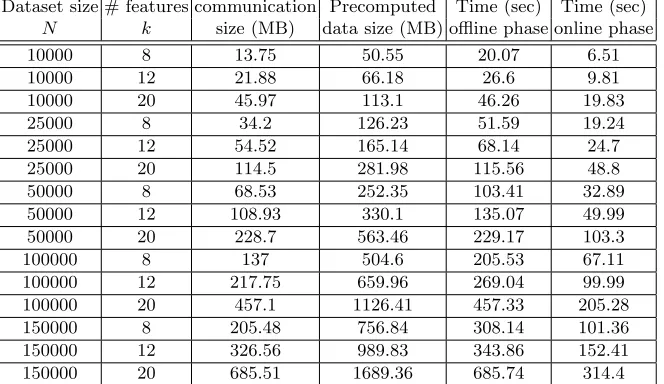
We present in this section a table (Table 1) summarizing the different measures we obtained during our experiments for n = 3 players. For this we considered datasets containing from 10000 to 1500000 points having 8, 12 or 20 features each.
Dataset size # features communication Precomputed Time (sec) Time (sec)
N k size (MB) data size (MB) offline phase online phase
10000 8 13.75 50.55 20.07 6.51
10000 12 21.88 66.18 26.6 9.81
10000 20 45.97 113.1 46.26 19.83
25000 8 34.2 126.23 51.59 19.24
25000 12 54.52 165.14 68.14 24.7
25000 20 114.5 281.98 115.56 48.8
50000 8 68.53 252.35 103.41 32.89
50000 12 108.93 330.1 135.07 49.99
50000 20 228.7 563.46 229.17 103.3
100000 8 137 504.6 205.53 67.11
100000 12 217.75 659.96 269.04 99.99
100000 20 457.1 1126.41 457.33 205.28
150000 8 205.48 756.84 308.14 101.36
150000 12 326.56 989.83 343.86 152.41
150000 20 685.51 1689.36 685.74 314.4
Table 1. Summary of the different measures (time, amount of exchanged data and amount of precomputed data) forn= 3 players.
B
Mask reduction algorithm
Algorithm 3 details our method, described in Section 3.3, for reducing the size of the secret shares. This procedure is used inside the classical MPC multiplication involving floating points.
Algorithm 3Mask reduction
Input: JzK+ and one tripletJνK+, withν= 0 modM.
Output: Secret shares for the same valuezwith smaller absolute values of the shares. 1: Each playerPicomputesui∈[−2η−1,2η−1) andvi∈Z, such thatzi=ui+ 2ηvi. 2: Each playerPibroadcastsvi+νi modM to other players.
3: The players computew= 1 n(
Pn
Fig. 1.Evolution of the cost function depending on the method
0 0.1 0.2 0.3 0.4 0.5 0.6 0.7
1 10 100 1000
Cost Function
Iteration number (logscale)
Standard GD cost Piecewise Approx cost MPC IRLS cost
Figure 1 shows the evolution of the cost function during the logistic regression as a function of the number of iterations, on a test dataset of 150000 samples, with 8 features and an acceptance rate of 0.5%. In yellow is the standard gradient descent with optimal learning rate, in red, the gradient descent using the piecewise linear approximation of the sigmoid function (as in [25]), and in green, our MPC model (based on the IRLS method). The MPC IRLS method (as well as the plaintext IRLS) method converge in less than 8 iterations, against 500 iterations for the standard gradient method. As expected, the approx method does not reach the minimal cost.
Fig. 2.Evolution of the F-score depending on the method
0 0.1 0.2 0.3 0.4 0.5 0.6 0.7 0.8 0.9 1
1 10 100 1000
Score
Iteration number (logscale)
Accuracy Standard F1-score Piecewise F1-score XOR IRLS F1-score
C
Approximation of functions by trigonometric
polynomial over the half period
Let f be a square-integrable function on the interval [−π/2, π/2] that is not necessarily smooth or periodic.
C.1 The approximation problem
Consider the set
Gn =
(
g(x) = a0
2 + n
X
k=1
aksin(kx) +
n
X
k=1
bkcos(kx)
)
of 2π-periodic functions and the problem
gn(x) = argming∈Gnkf−gkL2
[−π/2,π/2].
As it was observed in [7], if one uses the na¨ıve basis to write the solutions, the Fourier coefficients of the functionsgnare unbounded, thus resulting in numerical instability. It was explained in [21] how to describe the solution in terms of two families of orthogonal polynomials closely related to the Chebyshev polynomials of the first and second kind. More importantly, it is proved that the solution converges to f exponentially rather than super-algebraically and it is shown how to numerically estimate the solutiongn(x) in terms of these bases.
We will now summarize the method of [21]. Let
Cn=
1 √
2 ∪ {cos(kx) :k= 1, . . . , n}.
and let Cn be the R-vector space spanned by these functions (the subspace of even functions). Similarly, let
Sn={sin(kx) :k= 1, . . . , n},
and letSn be theR-span ofSn(the space of odd functions). Note thatCn∪Sn is a basis forGn.
C.2 Chebyshev’s polynomials of first and second kind
LetTk(y) fory∈[−1,1] be thekth Chebyshev polynomial of first kind, namely, the polynomial satisfying Tk(cosθ) = coskθ for all θ and normalized so that
Tk(1) = 1 (Tk has degree k). As k varies, these polynomials are orthogonal with respect to the weight functionw1(y) = 1/p1−y2. Similarly, letU
k(y) for
y∈[−1,1] be thekth Chebyshev polynomial of second kind, i.e., the polynomial satisfyingUk(cosθ) = sin((k+ 1)θ)/sinθand normalized so thatUk(1) =k+ 1. The polynomials {Uk(y)} are orthogonal with respect to the weight function
It is explained in [21, Thm.3.3] how to define a sequence{Th
k} of half-range Chebyshev polynomials that form an orthonormal bases for the space of even functions. Similarly, [21, Thm.3.4] yields an orthonormal basis{Uh
k}for the odd functions (the half-range Chebyshev polynomials of second kind). According to [21, Thm.3.7], the solutiongn to the above problem is given by
gn(x) =
n
X
k=0
akTkh(cosx) +
n−1
X
k=0
bkUkh(cosx) sinx,
where
ak =
2
π Z π2
−π
2
f(x)Tkh(cosx)dx,
and
bk =
2
π Z π2
−π
2
f(x)Ukh(cosx) sinxdx.
While it is numerically unstable to express the solutiongn in the standard Fourier basis, it is stable to express them in terms of the orthonormal basis {Th
k} ∪ {U h
k}. In addition, it is shown in [21, Thm.3.14] that the convergence is exponential. To compute the coefficientsak and bk numerically, one uses Gaus-sian quadrature rules as explained in [21,§5].
D
Proof of Theorem 1
We now prove Theorem 1, with the following methodology. We first bound the successive derivatives of the sigmoid function using a differential equation. Then, since the first derivative of the sigmoid decays exponentially fast, we can sum all its values for anyxmodulo 2π, and construct aC∞periodic function, which approximates tightly the original function over [−π, π]. Finally, the bounds on the successive derivatives directly prove the geometric decrease of the Fourier coefficients.
Proof. First, consider the σ(x) = 1/(1 +e−x) the sigmoid function over R.
σ satisfies the differential equation σ0 = σ−σ2. By derivating n times, we have σ(n+1)=σ(n)−Pn
k=0 n k
σ(k)σ(n−k)=σ(n)(1−σ)−Pn
k=1 n k
σ(k)σ(n−k). Dividing by (n+ 1)!, this yields
σ(n+1) (n+ 1)!
≤ 1
n+ 1
σ(n)
n! + n X k=1
σ(k)
k!
σ(n−k) (n−k)!
!
From there, we deduce by induction that for all n ≥ 0 and for all x ∈ R,
σ(n)(x) n!
≤1 and it decreases with n, so for alln≥1,
σ
(n)(x) ≤n!σ
Fig. 3.Odd-even periodic extension of the rescaled sigmoid
0 0.1 0.2 0.3 0.4 0.5 0.6 0.7 0.8 0.9 1
-6 -4 -2 0 2 4 6
oe(1,x) oe(3,x) oe(5,x)
The rescaled sigmoid functiong(αx) is extended by anti-periodicity from [−π 2;
π 2] to [π
2; 3π
2]. This graph shows the extended function for α = 1,3,5. By symmetry, the Fourier serie of the output function has only odd sinus terms: 0.5+P
n∈Na2n+1sin((2n+
1)x). Forα= 20/π, the first Fourier form a rapidly decreasing sequence: [6.12e-1, 1.51e-1, 5.37e-2, 1.99e-2, 7.41e-3, 2.75e-3, 1.03e-3, 3.82e-4, 1.44e-4, 5.14e-5, 1.87e-5, ...], which rapidly achieves 24 bits of precision. However, the sequence asymptotically decreases in
O(n−2) due to the discontinuity in the derivative in−π
2 , so this method is not suitable to get an exponentially good approximation.
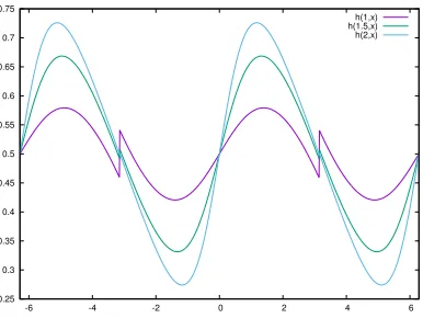
Fig. 4.Asymptotic approximation of the sigmoid via Theorem 1
0.25 0.3 0.35 0.4 0.45 0.5 0.55 0.6 0.65 0.7 0.75
-6 -4 -2 0 2 4 6
h(1,x) h(1.5,x) h(2,x)
Asαgrows, the discontinuity in the rescaled sigmoid functiong(αx)−x
We now construct a periodic function that should be very close to the derivative of hα: consider gα(x) = Pk∈Z
−α
(1+e−α(x−2kπ))(1+eα(x−2kπ)). By
sum-mation of geometric series, gα is a well-defined infinitely derivable 2π-periodic function over R. We can easily verify that for all x ∈ (−π, π), the difference
h0α(x)−21π −gα(x)
is bounded by 2α· P∞
k=1e
α(x−2kπ)≤ 2αe−απ
1−e−2πα, so by choos-ingα=Θ(log(1ε)), this difference can be made smaller than 2ε.
We suppose now that α is fixed and we prove that gα is analytic, i.e. its Fourier coefficients decrease exponentially fast. By definition,gα(x) =Pk∈Zσ(α(x− 2kπ)), so for allp∈N, gα(p)(x) = αp+1Pk∈Zσ(p+1)(αx−2αkπ), so
g
(p) α
∞≤
2αp+1(p+ 1)!. This proves that then-th Fourier coefficientc
n(gα) is ≤ minp∈N
2αp+1(p+1)!
np . This minimum is reached for p+ 1 ≈ n
α, and yields |cn(gα)|=O(e−n/α).
Finally, this proves that by choosingN≈α2=Θ(log(1/ε)2), theN-th term of the Fourier serie ofgα is at distance≤ ε2 ofgα, and thus fromh0α−21π. This bound is preserved by integrating the trigonometric polynomial (thegfrom the theorem is the primitive of gα), which yields the desired approximation of the
sigmoid over the whole interval (−π, π). ut
E
Honest but curious model
E.1 Honest but curious communication channels
The figures presented in this section represent the communication channels be-tween the players and the dealer in both the trusted dealer and the honest but curious models. Two types of communication channels are used: the private chan-nels, that correspond in practice to SSL channels (generally<20MB/s), and the public channels, corresponding in practice to TCP connections (generally from 100MB to 1GB/s). In the figures, private channels are represented with dashed lines, while public channels are represented with plain lines.
Figure 5 illustrates the connections during the offline phase of the MPC protocols. In the TD model, the dealer is the only one generating all the pre-computed data. He uses private channels to send to each player his share of the triplets (one-way arrows). In the HBC model, the players collaborate for the generation of the triplets. To do that, they need an additional private broadcast channel between them, that is not accessible to the dealer.
Figure 6 represents the communication channels between players during the online phase. The online phase is the same in both the TD and the HBC models and the dealer is not present.
E.2 Honest but curious algorithms
P1
P2
P3
Dealer
P1
P2
P3 Dealer
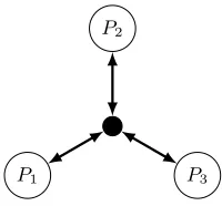
Fig. 5. Communication channels in the offline phase - The figure represents the communication channels in both thetrusted dealer model (left) and in thehonest but curious model (right) used during the offline phase. In the first model, the dealer sends the triplets to each player via a private channel. In the second model, the players have access to a private broadcast channel, shared between all of them and each player shares an additional private channel with the dealer. The private channels are denoted with dashed lines. The figure represents 3 players, but each model can be extended to an arbitrary numbernof players.
P1
P2
P3
Fig. 6. Communication channels in the online phase -The figure represents the communication channels (the same type for both the honest but curious and the trusted dealer model) used during the online phase. The players send and receive masked values via a public broadcast channel (public channels are denoted with plain lines). Their number, limited to 3 in the example, can easily be extended to a generic numbernof players.
generation of Beaver’s multiplicative triplets, while the second algorithm (Algo-rithm 5) details the generation of the triplets used in the MPC computation of a power function.
power in Algorithm 5). The dealer generates new additive shares for the result and sends these values back to each player via the private channel. This way, the players don’t know each other’s shares. Finally, the players, who know the common mask, can independently unmask their secret shares, and obtain their final share of the triplet, which is therefore unknown to the dealer.
Algorithm 4Honest but curious triplets generation
Output: Shares (JλK,JµK,JzK) withz=λµ.
1: Each playerPigeneratesai, bi, λi, µi (from the according distribution). 2: Each playerPishares with all other playersai,bi.
3: Each player computesa=a1+· · ·+anandb=b1+· · ·+bn. 4: Each playerPisends to the dealerai+λiandbi+µi. 5: The dealer computesa+λ,b+µandw= (a+λ)(b+µ).
6: The dealer createsJwK+ and sendswito playerPi, fori= 1, . . . , n. 7: PlayerP1 computesz1=w1−ab−aµ1−bλ1.
8: Playerifori= 2, . . . ncomputeszi=wi−aµi−bλi.
Algorithm 5Honest but curious triplets generation for the power function
Output: SharesJλKandJλ−α
K.
1: Each playerPigeneratesλi, ai (from the according distribution). 2: Each playerPishares with all other playersai.
3: Each player computesa=a1+· · ·+an.
4: Each playerPigeneratesziin a way thatPni=1zi= 0. 5: Each playerPisends to the dealerzi+aλi.
6: The dealer computesµλandw= (µλ)−α.