Matrix Computational Assumptions in Multilinear Groups
? ??Paz Morillo1, Carla R`afols2, and Jorge L. Villar1
1
Universitat Polit`ecnica de Catalunya, Spain
{paz.morillo,jorge.villar}@upc.edu 2
Universitat Pompeu Fabra, Spain
Abstract. We put forward a new family of computational assumptions, the Kernel Matrix Diffie-Hellman Assumption. Given some matrixAsampled from some distributionD, the kernel assump-tion says that it is hard to find “in the exponent” a nonzero vector in the kernel of A>. This family is the natural computational analogue of the Matrix Decisional Diffie-Hellman Assumption (MDDH), proposed by Escala et al. As such it allows to extend the advantages of their algebraic framework to computational assumptions.
Thek-Decisional Linear Assumption is an example of a family of decisional assumptions of strictly increasing hardness when kgrows. We show that for any such family of MDDH assumptions, the corresponding Kernel assumptions are also strictly increasingly weaker. This requires ruling out the existence of some black-box reductions between flexible problems (i.e., computational problems with a non unique solution).
Keywords: Matrix Assumptions, Computational Problems, Black-Box Reductions, Structure Preserving Cryptography
1
Introduction
It is commonly understood that cryptographic assumptions play a crucial role in the development of secure, efficient protocols with strong functionalities. For instance, upon referring to the rapid development of pairing-based cryptography, X. Boyen [8] says that “it has been supported, in no small part, by a dizzying array of tailor-made cryptographic assumptions”. Although this may be a reasonable price to pay for constructing new primitives or improve their efficiency, one should not lose sight of the ideal of using standard and simple assumptions. This is an important aspect of provable security. Indeed, Goldreich [16], for instance, cites “having clear definitions of one’s assumptions” as one of the three main ingredients of good cryptographic practice.
There are many aspects to this goal. Not only it is important to use clearly defined assumptions, but also to understand the relations between them: to see, for example, if two assumptions are equivalent or one is weaker than the other. Additionally, the definitions should allow to make accurate security claims. For instance, although technically it is correct to say that unforgeability of the Waters’ signature scheme [41] is implied by the DDH Assumption, defining the CDH Assumption allows to make a much more precise security claim.
A notable effort in reducing the “dizzying array” of cryptographic assumptions is the work of Escala
et al.[11]. They put forward a new family of decisional assumptions in a prime order groupG, theMatrix Diffie-HellmanAssumption (D`,k-MDDH). It says that, given some matrixA∈Z`q×ksampled from some
distributionD`,k, it is hard to decide membership in ImA, the subspace spanned by the columns ofA, in
the exponent. Rather than as new assumption, it should be seen as an algebraic framework for decisional assumptions which includes as a special case the widely usedk-Linfamily.
?Work supported by the Spanish research project MTM2013-41426-R and by a Sofja Kovalevskaya Award of
the Alexander von Humboldt Foundation and the German Federal Ministry for Education and Research.
??
This framework has some obvious conceptual advantages. For instance, it allows to explain all the members of the k-Lin assumption family (and also others, like the uniform assumption, appeared pre-viously in [13,14,40]) as a single assumption and unify different constructions of the same primitive in the literature (e.g., the Naor-Reingold PRF [35] and the Lewko-Waters PRF [29] are special cases of the same construction instantiated with the 1-Lin and the 2-Lin Assumption, respectively). Another of its advantages is that it avoids arbitrary choices and instead points out to a trade-off between efficiency and security (a scheme based on anyD`,k-MDDHAssumption can be instantiated with many different
assump-tions, some leading to stronger security guarantees and others leading to more efficient schemes). But follow-up work has also illustrated other possibly less obvious advantages. For instance, Heroldet al.[21] have used the Matrix Diffie-Hellman abstraction to extend the model of composite-order to prime-order transformation of Freeman [13] and to derive efficiency improvements which were proven to be impossible in the original model.3We believe this illustrates that the benefits of conceptual clarity can translate into concrete improvements as well.
The security notions for cryptographic protocols can be classified mainly in hiding and unforgeability ones. The former typically appear in encryption schemes and commitments and the latter in signature schemes and soundness in zero-knowledge proofs. Although it is theoretically possible to base the hiding property on computational problems, most of the practical schemes achieve this notion either information theoretically or based on decisional assumptions, at least in the standard model. Likewise, unforgeability naturally comes from computational assumptions (typically implied by stronger, decisional assumptions). Thus, a natural question is if one can find a computational analogue of theirMDDHAssumption which can be used in “unforgeability type” of security notions.
Most computational problems considered in the literature are search problems with a unique solution like the discrete logarithm orCDH. But unforgeability actually means the inability to produce one among many solutions to a given problem (e.g., in many signature schemes or zero knowledge proofs). Thus, unforgeability is more naturally captured by aflexible computational problem, namely, a problem which admits several solutions4. This maybe explains why several new flexible assumptions have appeared recently when considering “unforgeability-type” security notions in structure-preserving cryptography [2]. Thus a useful computational analogue of theMDDHAssumption should not only consider problems with a unique solution but also flexible problems which can naturally capture this type of security notions.
1.1 Our Results
In the followingG = (G, q,P), being Gsome group in additive notation of prime order q generated by P, that is, the elements ofGareQ=aP wherea∈Zq. They will be denoted as [a] :=aP. This notation
naturally extends to vectors and matrices as [v] = (v1P, . . . , vnP) and [A] = (AijP).
Computational Matrix Assumptions. In our first attempt to design a computational analogue of theMDDH Assumption, we introduce the Matrix Computational DH Assumption, (MCDH) which says that, given a uniform vector [v]∈Gk and some matrix [A], A← D
`,k for` > k, it is hard to extend [v]
to a vector inG`in the image of [A], Im[A]. Although this assumption is natural and is weaker than the
MDDHone, we argue that it is equivalent toCDH.
We then propose the Kernel Matrix DH Assumption (D`,k-KerMDH). This new flexible assumption
states that, given some matrix [A],A← D`,k for some` > k, it is hard to find a vector [v]∈G` in the
kernel ofA>. We observe that for some special instances ofD`,k, this assumption has appeared in the
lit-erature in [2,18,19,27,32] under different names, likeSimultaneous Pairing, Simultaneous Double Pairing (SDP in the following), Simultaneous Triple Pairing, 1-Flexible CDH, 1-Flexible Square CDH.Thus, the newKerMDH Assumption allows us to organize and give a unified view on several useful assumptions.
3 More specifically, we are referring to the lower bounds on the image size of a projecting bilinear map of [38]
which were obtained in Freeman model [13]. The results of [21] by-passed this lower bounds allowing to save on pairing operations for projecting maps in prime order groups.
4 In the cryptographic literature we sometimes find the term “strong” as an alternative to “flexible”, like the
This suggests that the KerMDHAssumption (and not the MCDH one) is the right computational ana-logue of theMDDHframework. Indeed, for any matrix distribution theD`,k-MDDH Assumption implies
the correspondingD`,k-KerMDHAssumption. As a unifying algebraic framework, it offers the advantages
mentioned above: it highlights the algebraic structure of any construction based on it, and it allows writing many instantiations of a given scheme in a compact way.
The power of Kernel Assumptions. At Eurocrypt 2015, ourKerMDHAssumptions were applied to design simpler QA-NIZK proofs of membership in linear spaces [26]. They have also been used to give more efficient constructions of structure preserving signatures [25], to generalize and simplify the results on quasi-adaptive aggregation of Groth-Sahai proofs [17] (given originally in [24]) and to construct a tightly secure QA-NIZK argument for linear subspaces with unbounded simulation soundness in [15]. The power of a KerMDH Assumption is that it allows to guarantee uniqueness. This has been used by Kiltz and Wee [26], for instance, to compile some secret key primitives to the public key setting. Indeed, Kiltz and Wee [26] modify a hash proof system (which is only designated verifier) to allow public verification (a QA-NIZK proof of membership). In a hash proof system for membership in some linear subspace ofGn
spanned by the columns of some matrix [M], the public information is [M>K], for some secret matrix K, and given the proof [π] that [y] is in the subspace, verification tests if [π]= [? y>K].
The core argument to compile this to a public key primitive is that given ([A],[KA]),A← D`,k and
any pair [y],[π], the previous test is equivalent toe([π>],[A]) =e([y>],[KA]), under theD`,k-KerMDH
Assumption. Indeed,
e([π>],[A]) =e([y>],[KA])⇐⇒e([π>−y>K],[A]) = [0]D`,k=-KerMDH⇒ [π] = [y>K]. (1) That is, although potentially there are many possible proofs which satisfy the public verification equation (left hand side of Equation (1)), the D`,k-KerMDH Assumption guarantees that only one of them is
efficiently computable, so verification gives the same guarantees as in the private key setting (right hand side of Equation (1)). This property is also used in a very similar way in [15] and also in the context of structure preserving signatures in [25]. In Section 6 we use it to argue that, of all the possible openings of a commitment, only one is efficiently computable,i.e.to prove computational soundness of a commitment scheme. Moreover, some previous works, notably in the design of structure preserving cryptographic primitives [1,2,3,31], implicitly used this property for one specific KerMDHAssumption: the Simultaneous (Double) Pairing Assumption.
On the other hand, we have already discussed the importance of having a precise and clear language when talking about cryptographic assumptions. This justifies the introduction of a framework specific to computational assumptions, because one should properly refer to the assumption on which security is actually based, rather than just saying “security is based on an assumption weaker thanD`,k-MDDH”.
A part from being imprecise, a problem with such a statement is that might lead to arbitrary, not optimal choices. For example, the signature scheme of [30] is based on the SDP Assumption but a slight modification of it can be based on theL2-KerMDHAssumption. If the security guarantee is “the assumption is weaker than 2-Lin” then the modified scheme achieves shorter public key and more efficient verification with no loss in security. Further, the claim that security is based on the MDDH decisional assumptions when only computational ones are necessary might give the impression that a certain tradeoff is in place when this is not known to be the case. For instance, Jutla and Roy [24] construct constant-size QA-NIZK arguments of membership in linear spaces under what they call the “Switching Lemma”, which is proven under a certainDk+1,k-MDDH Assumption. However, a close look at the proof reveals that in
fact it is based on the correspondingDk+1,k-KerMDHAssumption5. For these assumptions, prior to our
work, it was unclear whether the choice of largerk gives any additional guarantees.
5
To see this, note that in the proof of their “Switching Lemma” on which soundness is based, they use the output
of the adversary to decide iff ∈? ImA,A← RLk, by checking whether [f] is orthogonal to the adversary’s
output (equation (1), proof of Lemma 1, [24], full version), and where RLk is the matrix distribution of
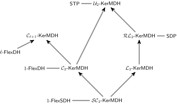
Strictly Increasing Families of Kernel Assumptions. An important problem is that it is not clear whether there are increasingly weaker families of KerMDHAssumptions. That is, some decisional assumptions families parameterized byklike thek-Lin Assumption are known to be strictly increasingly weaker. The proof of increasing hardness is more or less immediate and the term strictly follows from the fact that every two D`,k-MDDH and D`,eek-MDDH problems with ek < k are separated by an oracle
computing ak-linear map. For the computational case, increasing hardness is also not too difficult, but nothing is known about strictly increasing hardness (see Fig. 1). This means that, as opposed to the decisional case, prior to our work, for protocols based on KerMDH Assumptions there was no-known tradeoff between largerk(less efficiency) and security.
In this paper, we prove that the families of matrix distributions in [11],U`,k, Lk,SCk, Ck and RLk,
as well as a new distribution we propose in Section 7, thecirculant familyCIk,d, define families of kernel
problems with increasing hardness. For this we show a tight reduction from the smaller to the larger problems in each family. Our main result (Theorem 2) is to prove that the hardness of these problems is
strictly increasing. For this, we prove that there is no black-box reduction from the larger to the smaller problems in the multilinear generic group model. These new results correspond to the dotted arrows in Fig. 1.
D1-MDDH D2-MDDH D3-MDDH D4-MDDH · · ·
D2-KerMDH D3-KerMDH D4-KerMDH · · ·
/ / /
/ /
Fig. 1.Implication and separation results between Matrix Assumptions (dotted arrows correspond to the new results).
Having in mind that the computational problems we study in the paper are defined in a generic way, that is without specifying any particular group, the generic group approach arises naturally as the setting for the analysis of their hardness and reducibility relations. Otherwise, we would have to rely on specific properties of the representation of the elements of particular group families, not captured by the generic model.
The proof of Theorem 2 requires dealing with the notion of black-box reduction between flexible problems. A black-box reduction must work for any possible behavior of the oracle, but, contrary to the normal (unique answer) black-box reductions, here the oracle has to choose among the set of valid answers in every call. Ruling out the existence of a reduction implies that for any reduction there is an oracle behavior for which the reduction fails. This is specially subtle when dealing with multiple oracle calls. We think that the proof technique we introduce to deal with these issues can be considered as a contribution in itself and can potentially be used in future work.
Combining the black-box techniques and the generic group model is not new in the literature. For instance Dodis et al. [10] combine the black-box reductions and a generic model for the groupZ∗
n to show
some uninstantiability results for FDH-RSA signatures.
Theorem 2 supports the intuition that there is a tradeoff between the size of the matrix — which typi-cally results in less efficiency — and the hardness of theKerMDHProblems, and justifies the generalization of several protocols to different choices ofkgiven in [17,24,25,26].
bilinear groups. We unify these two constructions and we generalize to commit vectors of elements at each level Gr, for any 0≤r ≤m under the extension ofKerMDH Assumptions to the idealm-graded
encodings setting. In particular, whenm= 2 we recover in a single construction as a special case both the original Pedersen and Abeet al.commitments.
The (generalized) Pedersen commitment maps vectors in Gr to vectors in Gr+1, is perfectly hiding and computationally binding under any Kernel Assumption. In Section 6.3 we use it as a building block to construct a “group-to-group” commitment, which maps vectors in Gr to vectors in the same group
Gr. These commitments were defined in [3] because they are a good match to Groth-Sahai proofs. In [3],
two constructions were given, one in asymmetric and the other in symmetric bilinear groups. Both are optimal in terms of commitment size and number of verification equations. Rather surprisingly, we show that both constructions in [3] are special instances of our group-to-group commitment for some specific matrix distributions.
A New Family ofMDDHAssumptions of Optimal Representation Size. We also propose a new interesting family of Matrix distributions, the circulant matrix distribution, CIk,d, which defines new MDDH and KerMDH assumptions. This family generalizes the Symmetric Cascade Distribution (SCk)
defined in [11] to matrices of size`×k,`=k+d > k+ 1. We prove that it has optimal representation size dindependent of k among all matrix distributions of the same size. The case` > k+ 1 typically arises when one considers commitments/encryption in which the message is a vector of group elements instead of a single group element and the representation size typically affects the size of the public parameters.
We prove the hardness of the CIk,d-KerMDHProblem, by proving that theCIk,d-MDDHProblem is
generically hard ink-linear groups. Analyzing the hardness of a family of decisional problems (depending on a parameterk) can be rather involved, specially when an efficientk-linear map is supposed to exist. This is why in [11], the authors gave a practical criterion for generic hardness when`=k+ 1 in terms of irreducibility of some polynomials involved in the description of the problem. This criterion was used then to prove the generic hardness of several families ofMDDHProblems. To analyze the generic hardness of theCIk,d-MDDHProblem for anyd, the techniques in [11] are not practical enough, and we need some
extensions of these techniques for the case ` > k+ 1, recently introduced in [20]. However, we could not avoid the explicit computation of a large (but well-structured) Gr¨obner basis of an ideal associated to the matrix distribution. The new assumption can be used to instantiate the commitment schemes of Section 6 with shorter public parameters and improved efficiency.
2
Preliminaries
Forλ∈N, we write 1λ for the string of λones. For a setS, s←S denotes the process of sampling an
elementsfromS uniformly at random. For an algorithmA, we writez← A(x, y, . . .) to indicate thatA is a (probabilistic) algorithm that outputszon input (x, y, . . .). For any two computational problemsP1 andP2we recall thatP1⇒P2denotes the fact thatP1reduces toP2, and then ‘P1is hard’⇒‘P2is hard’. Thus, we will use ‘⇒’ both for computational problems and for the corresponding hardness assumptions. Let Gen denote a cyclic group instance generator, that is a probabilistic polynomial time (PPT) algorithm that on input 1λ returns a descriptionG= (G, q,P) of a cyclic groupG of orderqfor aλ-bit prime q and a generator P of G. We use additive notation for G and its elements areaP, for a∈ Zq
and will be denoted as [a] := aP. The notation extends to vectors and matrices in the natural way as [v] = (v1P, . . . , vnP) and [A] = (AijP). For a matrixA ∈ Z`q×k, ImA denotes the subspace of Z`q
spanned by the columns ofA. Thus, Im[A] is the corresponding subspace ofG`.
2.1 Multilinear Maps
In the case of groups with a bilinear map, or more generally with ak-linear map fork≥2, we consider a generator producing the tuple (ek,G1,Gk, q,P1,Pk), whereG1,Gk are cyclic groups of prime-orderq,
Pi is a generator of Gi andek is a non-degenerate efficiently computable k-linear map ek :Gk1 →Gk,
For any fixedk≥1, letMGenk be a PPT algorithm that on input 1λ returns a description of a graded
encoding MGk = (e,G1, . . . ,Gk, q,P1, . . . ,Pk), where G1, . . . ,Gk are cyclic groups of prime-order q,
Pi is a generator of Gi and e is a collection of non-degenerate efficiently computable bilinear maps
ei,j : Gi×Gj → Gi+j, for i+j ≤ k, such that e(Pi,Pj) = Pi+j. For simplicity we will omit the
subindexes ofewhen they become clear from the context. SometimesG0is used to refer toZq. For group
elements we use the following implicit notation: for alli= 1, . . . , k, [a]i:=aPi. The notation extends in
a natural way to vectors and matrices and to linear algebra operations. We sometimes drop the index when referring to elements inG1,i.e., [a] := [a]1=aP1. In particular, it holds thate([a]i,[b]j) = [ab]i+j.
Additionally, for the asymmetric case, let AGen2 be a PPT algorithm that on input 1λ returns a description of an asymmetric bilinear groupAG2= (e,G,H,T, q,P,Q), whereG,H,Tare cyclic groups of prime-orderq,P is a generator ofG, Qis a generator ofHande:G×H→Tis a non-degenerate, efficiently computable bilinear map. In this case we refer to group elements as: [a]G :=aP, [a]H :=aQ
and [a]T :=ae(P,Q).
3
A Generic Model For Groups With Graded Encodings
In this section we describe a (purely algebraic) generic model for the graded encodings in order to obtain meaningful results about the hardness and separations of computational problems. The model is an adaptation of Maurer’s generic group model [33,34] including thek-graded encodings, but in a completely algebraic formulation that follows the ideas in [5,12,20]. Since thek-graded encodings functionality implies thek-linear group functionality, the former gives more power to the adversaries or reductions working within the corresponding generic model. This in particular means that non-existential results proven in the richer k-graded encodings generic model also imply the same results in the k-linear generic group model. Therefore, here we consider the former model. However, for the sake of simplicity, in other sections of this paper we will use the more common name ‘multilinear generic group model’ to refer to thek-graded encodings generic model.
In a first approach we consider Maurer’s model adapted to the graded encodings functionality, but still not phrased in a purely algebraic language. In this model, an algorithm Agen does not deal with proper group elements [y]a ∈Ga, but only with labels (Y, a), and it has access to an additional oracle
Ogeninternally performing the group operations, so thatAgencannot benefit from the particular way the group elements are represented.
As we need to handle elements in different groups, we will use the shorter vector notation [x]a =
([x1]a1, . . . ,[xα]aα) = (x1Pa1, . . . , xαPaα)∈Ga1× · · · ×Gaα. Note that the length of a vector of indices a is denoted by a corresponding Greek letterα. We will also use a tilde to denote variables containing only non-group elements (i.e., elements not belonging to any ofG1, . . . ,Gk).
3.1 The Generic Model for Algorithms Without Additional Oracle Access
We first address the simple case of algorithms without access to additional oracles (i.e., only the oracle associated to the generic model will be considered).
Definition 1 (Generic Algorithm). An algorithm Agen is called generic (in the sense of the generic
model for k-graded encodings) if, on start it receives as input some labels (X1, a1), . . . ,(Xα, aα)
repre-senting the vector of group elements[x]a. The stateful oracle Ogen implementing the k-graded encodings
initially holds a table T containing these group elements along with their corresponding labels. That is, every entry in T has the form ([xi]ai,(Xi, ai)). Additionally, A
gen can receive some extra inputs
cor-responding to non-group elements, including for instance some size parameters. We denote these extra inputs as xe, which can be considered as a bit string. For each group Ga, a = 1, . . . , k, two additional
labels (0, a),(1, a), corresponding to the neutral element and the generator, are implicitly given to Agen.
The size of the groupsqis also implicitly given to Agen.
– GroupOp((Y1, a),(Y2, a)): group operation inGa for two previously issued labels in Ga resulting in a
new label(Y3, a)inGa. In addition,Ogen performs the real operation [y3]a = [y1]a+ [y2]a (using the
group elements stored inT) and adds the new entry ([y3]a,(Y3, a))toT. – GroupInv((Y, a)): idem. for group inversion in Ga.
– GroupPair((Y1, a),(Y2, b)): bilinear map for two previously issued labels in Ga and Gb, a+b ≤ k,
resulting in a new label(Y3, a+b)inGa+b. The corresponding new entry is added to T.
– GroupEqTest((Y1, a),(Y2, a)): test two previously issued labels inGa for equality of the corresponding
group elements, resulting in a bit (1 = equality).
Every badly formed query (for instance, containing a label not previously issued by the oracle or as an input toAgen) is answered with a special rejection symbol⊥.
In the end, Agen outputs another set of labels(Y
1, b1), . . . ,(Yβ, bβ)(given at some time by the generic
model oracleOgen) corresponding to group elements[y]
b= ([y1]b1, . . . ,[yβ]bβ), along with some non-group
elements, denoted as ey, which is also a bit string. The final state of the oracle Ogen is defined to be the
part of the internal table T consisting of the labels (Y1, b1), . . . ,(Yβ, bβ) and their corresponding group
elements[y]b.
Observe that all valid queries toOgen can be properly managed by it with the help of thek-graded encodings. Indeed, all the group indices in the labels are forced to belong to the set{1, . . . , k}.
The generic algorithmAgen described above is not a proper algorithm, because it actually does not perform any computation with group elements but it only instructs the oracle Ogen to carry out the computations. However, one can obtain a real algorithm Afrom Agen and a front-end in the following way:
1. The front-end interceptsA’s input, replaces the group elements by labels and internally stores these group elements.
2. Agenstarts its execution and the front-end emulates the oracleOgenfor it, thus performing the actual computations with the internally stored group elements.
3. The front-end collects the output given byAgen at the end of the execution and replaces the labels by the corresponding group elements to obtain the intended output forA. If the front-end detects an invalid label (not previously issued byOgenas the response of some oracle query), then the execution is aborted.
There is a technical problem with the non-group elements, since the value of xe could give some unintended information toAgenabout x
1, . . . , xα. For instance, we could setxe=x1. In order to obtain meaningful results, in the following definition we capture some extra requirements for the generation of the inputs ofAgen.
Definition 2 (Bounded Polynomial Source). We call D a bounded polynomial source of degree d
and withδparameters if there exists a polynomial mapf :Zδ
q→Zαq of total degreedsuch thatD outputs
the evaluation off at a uniformly distributed random point (t1, . . . , tδ)∈Zδq.6
Additionally, we consider the case that D depends on an auxiliary input τ ∈ {0,1}∗. In this case we
require that for every value ofτ,Dτ is a bounded polynomial source of degree≤dand for a fixed δ(i.e.,
dandδare independent ofτ). When needed, we will refer to the polynomial map instance corresponding toDτ explicitly as fτ. However, for simplicity we will usef if it causes no ambiguity.
We will consider from now on that the input of a generic algorithm comes from a bounded polynomial sourceD (i.e., the outputx ofD is conveniently encoded as group elements [x]a), where the auxiliary
input consists of the non-group elementsx. This extra requirement could be seen as a serious limitatione of the generic model. However, the way the inputs are sampled is typically part of the specification of the problem to be solved byAgen. In particular, kernel problems dealt with in this paper are particular examples of bounded polynomial sources, where the auxiliary information consists of the size parameters kand`of the associated matrix distribution.
6
Following the usual step in generic group model proofs (see for instance [5,11,20]), we use poly-nomials as labels to group elements. Namely, labels in Ga are polynomials in Zq[X], where the
al-gebraic variables X = (X1, . . . , Xα) are just formal representations of the group elements in the
in-put of Agen. We emphasize that the degree of these input labels (as polynomials in Z
q[X]) is one.
Now in the oracle side, group operations are replaced by polynomial operations in the labels. Indeed,
GroupOp((Y1, a),(Y2, a)) = (Y1 +Y2, a), GroupInv((Y, a)) = (−Y, a) and GroupPair((Y1, a),(Y2, b)) = (Y1Y2, a+b). It is easy to see that for any valid label (Y, a), degY ≤ a. It clearly holds for the in-put group elements (since degX1 = · · · = degXα = 1 and all a1, . . . , aα ≥ 1), and the inequality is
preserved byGroupOp, GroupInv and GroupPair. In particular, the oracle call GroupPair((Y1, a),(Y2, b)) results in the label (Y1Y2, a+b). Then the input inequalities degY1≤aand degY2≤bimply the output inequality deg(Y1Y2) = degY1+ degY2 ≤ a+b. On the other hand, GroupOp((Y1, a),(Y2, a)) outputs (Y1+Y2, a) and deg(Y1+Y2)≤max(degY1,degY2)≤a. The same argument applies toGroupInv.
This polynomial-based labelling is well-defined, since the group element [y]a corresponding to a label
(Y, a) is exactly [Y(x1, . . . , xα)]a. Therefore different group elements always receive different labels. On
the other hand, two different labels (Y1, a) and (Y2, a) can be associated to the same group element [y]a, thus implying that the polynomialY1−Y2∈Zq[X] vanishes at the point (x1, . . . , xα). These label
collisions can occur either predictably, because of the way the point (x1, . . . , xα) is sampled, or by the
unexpected ability of Agen to find them. An example of predictable collisions occurs when the source D produces x1 =t and x2 = −t. Then, the oracle call GroupEqTest((X1, a),GroupInv((X2, a))) always results in 1. This is something predictable byAgenitself, assuming that it knows the mapf. Notice that Agencan predict all answers given by the oracle Ogen except for someGroupEqTest queries, that we call nontrivial.
Definition 3 (Nontrivial Equality Test Queries).Given a bounded polynomial sourceD with poly-nomial mapf :Zδ
q →Zαq of total degreedand auxiliary informationeτ∈ {0,1}
∗, and a generic algorithm
Agen, the oracle callGroupEqTest((Y
1, a),(Y2, a))is called nontrivial (for some specific value ofeτ) if and
only if Y1◦feτ 6= Y2◦feτ, as polynomials in Zq[T], where T = (T1, . . . , Tδ) are the parameters of the
bounded polynomial source D.
Here we will assume that the description of the mapf is fixed, and it can be used byAgen, and also the auxiliary input τe is given to Agen. Clearly this would not be the case when dealing with decision problems, where a distinguisher aims at telling apart two possible problem instance distributions (i.e., there are two candidates forf). Nevertheless here we restrict ourselves to the study of search problems. At this point all the informationAgencan obtain from the oracleOgen is via the nontrivialGroupEqTest queries. Indeed,Agen can perform itself the same polynomial operations in the labels asOgen, and it can use the mapf to predict the answers to the trivialGroupEqTestqueries.
We now introduce a “purely algebraic” version of the generic model by slightly modifying the oracle Ogen. To distinguish the two models, we denote the modified oracle as Opa-gen. In this new model we need to specify a bounded polynomial source which provides the input forAgen.
Definition 4 (Purely-Algebraic Generic Algorithm).7Given a bounded polynomial sourceD with auxiliary inputxe∈ {0,1}∗and polynomial mapf :Zδ
q →Zαq of total degreed, an algorithmAgen is called
generic (in the sense of the purely-algebraic generic model fork-graded encodings) with respect toD if it follows Definition 1, except that it receives as inputxeand the output ofD (this was not required before) and it has access to the oracleOpa-gen, which differs fromOgen in that:
– The internal tableT now contains entries(Xi◦fex,(Xi, ai)), where the group element has been replaced
by the “internal” polynomialXbi=Xi◦fex∈Zq[T].
– For valid labels GroupEqTest((Y1, a),(Y2, a))outputs 1 if and only if the corresponding internal
poly-nomials are equal, that is, Yb1=Yb2, as polynomials inZq[T].
– Opa-gen does not store any group element and it does not perform any real group operation. Instead,
once Agen has finished its execution by outputting the labels(Y
1, b1), . . . ,(Yβ, bβ), Opa-gen samples a
7
random point t ∈ Zδ
q (in the same way as D would did it) and then it evaluates the corresponding
internal polynomials Yb1, . . . ,Ybβ extracted from T at the sampled point t ∈Zδq, that is y =Yb(t) =
Y ◦f
e
x(t). Finally, Opa-gen computes the output group elements[y]b from their discrete logarithmsy.
Notice that in the plain (non-algebraic) generic model t is also sampled from D, but at the very beginning of the game. Therefore, it is self-evident that the representation of the group elements is irrelevant forAgenin the purely-algebraic model, since the group elements themselves are never created. Is can be proved that, with this change in the generic model, the behavior of Agen can only change negligibly, assuming thatxcomes from a bounded polynomial source andqis exponentially large. This is just a standard argument used in proofs in the generic group model. The difference between the original model and its purely algebraic reformulation is typically upper-bounded by using Schwartz-Zippel Lemma and the union bound, as shown for instance in [5,12,20]. More precisely,
Lemma 1. Let Agen be a generic algorithm receiving inputs from a bounded polynomial sourceD with
auxiliary input xe∈ {0,1}∗ and polynomial map f : Zδ
q →Zαq of total degree d. Then, for exponentially
largeq, the difference between the success probabilities ofAgen in the generic model fork-graded encodings
interacting with eitherOgen orOpa-genis negligible. This holds even when
e
xis correlated with the random tape ofAgen.
Proof. The only way in which the plain generic model and its purely algebraic counterpart can differ is whenAgen makes a nontrivialGroupEqTest query. Namely, for specific values of
e
xand the random tape of Agen, the algorithm is able to find two valid labels (Y
1, a) and (Y2, a) such that their corresponding internal polynomials are different, that isY1◦fex6=Y2◦fxeas polynomials inZq[T], while the answer of GroupEqTest((Y1, a),(Y2, a)) is 1 in the plain (non-algebraic) generic model. Equivalently,Agen is able to find a nonzero polynomialZ =Y1◦fex−Y2◦fex= (Y1−Y2)◦fex ∈Zq[T] that vanishes at the random
pointt= (t1, . . . , tδ) internally sampled byD.
For every individual choice ofexand the random tape ofAgen, the probability that this event occurs is at most dkq by Schwartz-Zippel Lemma, because deg((Y1−Y2)◦fxe)≤deg(Y1−Y2) degfex≤kd. Finally, if
Qgenis the number of queries toOgen made byAgen other thanGroupEqTest queries, thenAgenreceives at mostQgen+α+ 2k different labels (including the input labels and the implicitly given ones). By a straightforward hybrid argument (or simply using the union bound) the difference between the success probabilities ofAgen in the two models is upper bounded by
Pr[Bad]≤
Q
gen+α+ 2k 2
dk
q ,
which is negligible ifqis exponentially large. Notice that this bound applies to every choice ofxeand the random tape ofAgen, which means in particular that the result holds even if these two objects are not
independent random variables. ut
We stress that this bound is computed for any value of ex and, by Definition 2, the parameters (t1, . . . , tδ) are sampled independently ofx. This captures the fact thate Agen cannot receive unintended
information aboutx1, . . . , xαvia the non-group element inputs.
Once we have proved that generic algorithms receiving inputs from a bounded polynomial source performs similarly in both the original generic model and the purely-algebraic one, we now assume that both models are the same, and choose the simplest one: the purely-algebraic generic model. The simplicity of the model comes from the fact thatAgen receives absolutely no information about the group element inputs (x1, . . . , xα). ActuallyAgendoes not perform the computations but it just instructsOpa-gen to do
so. Namely, from the particular values ofexand a random tape,Agencomputes the polynomialsY
1, . . . , Yβ
and gives them to the oracle (incrementally, via the oracle calls). ThenOpa-gensamples (x
1, . . . , xα) from
D given xe and evaluates the polynomials at the sampled point. Nevertheless, Agen still computes the non-group elements in the output y. But thene yecan only depend on xe and the random tape ofAgen, which are the only inputs received byAgen (in the purely algebraic model the oracle Opa-gen gives no information toAgen). Then, for a fixed value of
e
xand for every choice of the random tape ofAgen,Agen runs deterministically, and the polynomials Y1, . . . , Yβ are used for all possible choices of (x1, . . . , xα)
(drawn fromD
e
3.2 Algebraic Algorithms Without Oracle Access
We now capture the previous considerations into a formal definition of algebraic algorithm (no to be confused with a generic algorithm).
Definition 5 (Algebraic Algorithm).An algorithmAalgis called algebraic (in the sense of the generic
model fork-graded encodings) if on start it receives as input the group elements[x1]a1, . . . ,[xα]aα and an
auxiliary inputxe(the size of the groups qand the group generators [1]1, . . .[1]k are also given implicitly
toAalg), and its output([y
1]b1, . . . ,[yβ]bβ,y)e is computed by the following two stages:
1. Fromxeand the random tape, Aalg computes polynomials Y
1, . . . , Yβ ∈Zq[X]such that degYi ≤bi.
In additionAalg computes the auxiliary output
e
y.
2. Aalg uses the computed polynomials and thek-graded encodings to compute[y
1]b1, . . . ,[yβ]bβ such that yj=Yj(x1, . . . , xα), for j= 1, . . . , β.
Observe that Aalg is an actual algorithm with a very restricted structure, and it do not require the assistance of any oracle, as it makes use of the realk-graded encodings. However algebraic algorithms are in some sense equivalent to generic algorithms as stated below.
Lemma 2. Given a generic algorithmAgenas described in Definition 1 with inputs(X
1, a1), . . . ,(Xα, aα)
andex, and a bounded polynomial sourceD, as described in Definition 2, with auxiliary inputxe∈ {0,1}∗
and polynomial mapf :Zδ
q →Zαq of total degree d, there exists an algebraic algorithmAalg that produces
the same outputs as Agen in the purely-algebraick-graded encoding generic model (i.e., interacting with
the oracleOpa-gen) with input group elements sampled fromD.
Proof. Aalgreceives the inputs [x
1]a1, . . . ,[xα]aα and an auxiliary inputx, where (xe 1, . . . , xα) are sampled
from D
e
x. Then it simulates the oracle Opa-gen for Agen following Definition 4. Namely, Aalg starts the
execution ofAgenwith the inputs ((X
1, a1), . . . ,(Xα, aα),ex), wherea1, . . . , aα are the values in the
defi-nition ofAgen andX = (X
1, . . . , Xα) are algebraic variables. Then all the oracle queries made by Agen
are simulated in a straightforward way, by performing the corresponding polynomial operations in the labels, except for theGroupEqTestqueries. A valid queryGroupEqTest((Y1, a),(Y2, a)) is answered with 1 if and only if the corresponding internal polynomials are equal, namelyY1◦fex=Y2◦fex as polynomials
in Zq[T]. This first stage of Aalg ends up by collecting the output polynomials Y1, . . . , Yβ ∈Zq[X] and
the auxiliary outputey given byAgen. The second stage follows exactly Definition 5.
The simulation performed byAalgis perfect and it fulfils the requirements given in Definition 5, since the values of [x1]a1, . . . ,[xα]aα are only used in the second stage. The degree requirement degYi≤bi as polynomials inZq[X] directly comes from the above discussion about the degrees of the polynomial labels
across the oracle calls. Recall that degXi= 1 by definition, as the labels are polynomials in Zq[X]. ut
As a consequence, for any generic algorithm Agen in the original (i.e. non-algebraic) generic model fork-graded encodings in exponentially large groups receiving inputs from a bounded polynomial source, there exists an algebraic algorithmAalg with identical performance except for a negligible probability. Moreover, the very restricted structure of an algebraic algorithm allows us to state the following technical result.
Lemma 3. Let Aalg be an algebraic algorithm. Let ([x]
a,x)e and ([y]b,ey) respectively be the input and
output of Aalg. Then, for every choice of
e
x∈ {0,1}∗ and any choice of the random tape of Aalg, there
exist polynomials Y1, . . . , Yβ ∈Zq[X] of degree upper bounded by b1, . . . , bβ such that y=Y(x), for all
x∈Zα
q, where Y = (Y1, . . . , Yβ). Moreover, yeonly depends on exand the random tape of Aalg (i.e., it
does not depend onx).
Proof. The proof of the lemma comes straightforward from the structure given in Definition 5. Indeed, the polynomialsY1, . . . , Yβ and the auxiliary outputyeare exactly the ones computed byAalg in the first
stage of its execution. Thus, they directly fulfil the three requirements: degYi ≤bi, yi =Yi(x1, . . . , xα)
In addition, algebraic algorithms and bounded polynomial sources can be related in the following way:
Lemma 4. The composition of an algebraic algorithm, that only outputs group elements, with a bounded polynomial source is another bounded polynomial source.
Proof. LetAalgbe an algebraic algorithm with input ([x]
a,x) and output ([e y]b). Let us assume thatxis
produced by a bounded polynomial sourceDwith auxiliary inputτ and polynomial mapfτ :Zδq →Zαq
of total degreed. For any choice ofτ,xeand the random tape ofAalg, according to Lemma 3 there exists a polynomial map Y = (Y1, . . . , Yβ) of degree at most k (since for all j = 1, . . . , β, degYj ≤ bj ≤ k)
such thaty=Y(x), for allx∈Zα
q. Therefore,y=Y ◦fτ(t) for allt∈Zδq. This actually shows thaty
behaves exactly as the output of a bounded polynomial source with auxiliary inputτ0= (τ,x,e $), where $ denotes the random tape ofAalg, and polynomial mapf0
τ0:Zδq →Zqβ such thatf0 =Y ◦f. The degree
off0 is upper bounded by degY ◦f ≤degYdegf ≤kd. ut
3.3 A Comment on Generic Hardness
As usual, the proposed generic model reduces the analysis of the hardness of some problems to solving a merely algebraic problem related to polynomials. As an example, consider a computational problemP which instances are entirely described by some group elements in the base groupG1, [x]← P.InstGen(1λ),
and its solutions are also described by some group elements [y]b ∈ P.Sol([x]). We also assume that
P.InstGen just samples x by evaluating polynomial functions of constant degree at a random point. Then,P is generically hard if and only if for all (randomized) polynomialsY1, . . . , Yβ ∈Zq[X] of degrees
upper bounded byb1, . . . , bβ respectively,
Pr([y]b∈ P.Sol([x]) : [x]← P.InstGen(1λ),y=Y(x))∈negl(λ)
whereY = (Y1, . . . , Ym) and the probability is computed with respect the random coins of the instance
generator and the randomized polynomials.8 In a few words, this means that the set P.Sol([x]) cannot be hit by polynomials of the given degree evaluated atx.
3.4 Adding Oracles to the Model
The previous model extends naturally to algorithms with oracle access (e.g., black-box reductions) but only when the oracles fit well into the generic model. Let us introduce the notion of an algebraic algorithm AO, with oracle access toO.
Definition 6 (Algebraic Oracle Algorithm). An oracle algorithm AO is called algebraic (in the
sense of the purely-algebraic generic model for k-graded encodings) if on start it receives as input the group elements[x]a= ([x1]a1, . . . ,[xα]aα)and an auxiliary input xe. Next, it sets [z]c = [x]a and ez=ex
as inputs for the first iteration and proceeds as follows:
1. From ze and the random tape, it computes polynomials Y1, . . . , Yβ, U1, . . . , Uδ ∈ Zq[Z] such that
degYi ≤ bi and degUi ≤ di, for some fixed vectors of indices (b1, . . . , bβ) and (d1, . . . , dδ).9 In
addition it computes some non-group elements (ey,u,e stopg).
2. The algorithm uses the polynomials Y1, . . . , Yβ, U1, . . . , Uδ and the k-graded encodings to compute
[y1]b1, . . . ,[yβ]bβ,[u1]d1, . . . ,[uδ]dδ such that yi = Yi(z), for i = 1, . . . , β and uj = Uj(z), for j = 1, . . . , δ.10
8
We can similarly deal with problems with non-group elements both in the instance description and the solution, but this would require a more sophisticated formalization, in which both the polynomials and the non-group elements in the solution could depend on the non-group elements in the instance, but in an efficient way.
9 All the index vectors except fordandecan indeed change in each iteration. 10
These computations must be always possible, which imposses some limitations in the degree and the particular form of the polynomials, depending on the group indicesc1, . . . , cγ. For instance, ifc1 =kthen Z1 can only
appear in a linear terms in the polynomials. These limitations can be easily modelled by assigning to each formal variableZi a degree ciand then allowing only a polynomialYj of total degree at mostdj for a group
element [yj]dj. However, this notion of degree is not the one that we need in Schwartz-Zippel lemma. Thus, we
3. Ifstopg = 1 then the algorithm finishes its execution by outputting([y1]b1, . . . ,[yβ]bβ,ey).
11
4. Otherwise, the oracleO is queried with ([u1]d1, . . . ,[uδ]dδ,u)e . Let the answer given by the oracle be
([v1]e1, . . . ,[v]e,v)e, for some fixed vector of indices (e1, . . . , e).
5. The algorithm sets[z]c= ([y]b,[v]e)andez= (y,e ev)as inputs for the next iteration, and continues.
Observe that the algebraic oracle algorithm is split into sections between oracle calls. All state information between sections is contained in the iteration input/output variables [z]c andez. Each section is required
to behave as a standalone algebraic algorithm, but no special requirement is imposed to the oracle O. However, to make this definition useful, the oracle must preserve the algebraic properties of the different sections, like properly separating group elements from non-group elements. Indeed, a completely arbitrary oracle (specified in the plain model) could have access to the internal representation of the group elements, and then it could leak some information about the group elements that is outside the generic model. Thus, we will impose the very limiting constraint that the oracles are also “algebraic”, meaning that the oracle’s input/output behavior respects the one-wayness of the graded encodings,12 and they only perform “polynomial operations” on the group elements.
Definition 7 (Algebraic Oracle). Let ([u]d,eu) and ([v]e,ev) respectively be a query to an oracle O
and its corresponding answer, whereeuandev contain the respective non-group elements. The oracleO is called algebraic if for any choice of euthere exist polynomials V1, . . . , V ∈Zq[U,R],R = (R1, . . . , Rρ),
of constant degree (i.e., not depending onue,qor any security parameter) such that
– for the specific choice of eu, vi = Vi(u,r), i = 1, . . . , , for all u ∈ Zq and r ∈ Zρq, where r =
(r1, . . . , rρ) are random parameters defined and uniformly sampled by the oracle,
– ev does not depend on u,r (thus, r can only have influence in the group elements in the answer),
– the polynomial Vj does not depend on any variable Ui such that ej < di (in order to preserve the
one-wayness of the graded encodings).
The parametersr capture the behavior of an oracle solving a problem with many solutions (called here a “flexible” problem), and they are independent across different oracle calls, meaning that the oracle is stateless. Observe that the first two requirements in the definition mean thatv depends algebraically on u,rand no extra information about u,r can be leaked throughev. Removing any of these requirements from the definition results in that a generic algorithm using such an oracle will no longer be algebraically generic. Also notice that after a call to an algebraic oracle, there is no guarantee that labels (Y, a) fulfil the bound degY ≤a.
Although the notion of algebraic oracle looks very limiting, it is general enough for our purposes. Notice for example that the notion of algebraic oracle excludes a Discrete Logarithm oracle, as it destroys the one-wayness property of the graded encodings, but on the other hand, oracles solving CDH or the Computational Bilinear Diffie-Hellman problem fit well in the definition. As an example, consider an oracle solving CDH in G1. The input here is ([u]d,eu) = ([u1]1,[u2]1) while the output is ([v]e,ev) =
([u1u2]1). This oracle needs no non-group elements and there are also no internal parameters involved, since CDH is not a flexible problem. Observe that the oracle can be modelled by a single polynomial V1(U,R) = V1(U1, U2) = U1U2. Moreover, degV1 = 2 > b1 = 1, which is something that is beyond the limitations of the generic model fork-linear encodings. But this just means that theCDHoracle is performing a nontrivial task.
Regarding the way an algebraic oracle chooses the internal parameters, we restrict ourselves to the random uniform case, in whichr is sampled uniformly at random independently in every query to the oracle. Notice that other interesting probability distributions can be easily captured by properly choosing the polynomialsV1, . . . , V. Algebraic oracles can also be related to bounded polynomial sources:
Lemma 5. The composition of an algebraic oracle with a bounded polynomial source is another bounded polynomial source.
11
Ifstop = 1, normallyg euanduare empty, or they contain dummy values. 12
Proof. LetOalg be an algebraic oracle with input ([u]
a,eu) and output ([v]b). Let us assume thatu is
produced by a bounded polynomial sourceDwith auxiliary inputτ and polynomial mapfτ :Zδq →Zαq
of degree d. For any choice of τ and u, according to Definition 7 there exists a polynomial mape V = (V1, . . . , Vβ) of constant degree dO such thatv =V(u,t), for allu∈Zαq and r∈Zρq, wherer denotes
the internal parameters of the oracle. Therefore, v=V(fτ(t),r) for allt∈Zδq andr∈Zρq. This shows
thatv behaves exactly as the output of a bounded polynomial source with auxiliary inputτ0= (τ,u) ande polynomial mapfτ00 :Zδq×Zρq →Zβq such thatf0(t,r) =V(fτ(t),r). The degree off0 is upper bounded
by degV ◦f ≤degVdegf ≤dOd. ut
Now we can state the generalization of Lemma 3 for oracle algorithms. It is actually a ‘composition theorem’ meaning that combining an algebraic (oracle) algorithm with an algebraic oracle produces another (weak) algebraic algorithm. We said ‘weak’ because the degrees of the corresponding input-output polynomials no longer satisfy the constraint degY ≤ a (since the algebraic oracle typically performs nontrivial tasks, like in the CDH example). We actually can only guarantee that the degrees of the polynomials are upper bounded by constants (i.e., the bounds are independent of the security parameter). Furthermore, we need to impose that the number of oracle calls is upper bounded by a constantQ. Observe that the degree of the polynomials could grow exponentially in the number of oracle calls (e.g., using the answer of the previous call in the next oracle query for the oracleO computing [v]1 = [u2]1 yields polynomials of degree 2Q).
Lemma 6. Let AO be an algebraic oracle algorithm (as given in Definition 7), making a constant13
bounded number of callsQto an algebraic oracleO. Let([x]a,ex)and([y]b,ey)respectively be the input and
output ofA. Then, for every choice ofexand the random tape, there exist polynomials of constant degree
Y1, . . . , Yβ∈Zq[X,R1, . . . ,RQ], such thaty=Y(x,r1, . . . ,rQ), for all inputs, whereY = (Y1, . . . , Yβ),
and r1, . . . ,rQ are the parameters introduced in Definition 7 for the Q queries. Moreover, ey does not
depend onxorr1, . . . ,rQ.
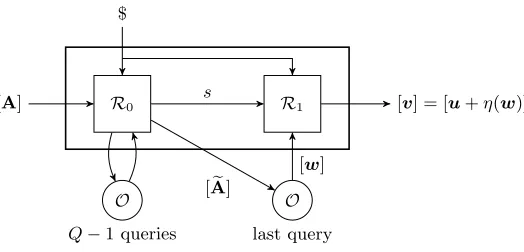
Proof. We proceed by induction inQ. The first induction step,Q= 0, follows immediately from Lemma 3, becauseAOis just an algebraic algorithm (without oracle access). ForQ≥1, we splitAOinto two sections AO
0 andA1, separated exactly at the last query point (see Figure 2). Let ([s]c,es) be the state information
(group and non-group elements) thatAO
0 passes to A1, ([u]d,eu) be the Q-th query to O, and ([v]d,ev)
be its corresponding answer. We assume that AO
0 and A1 receive the same random tape, $, (perhaps introducing some redundant computations inA1). Observe that the output ofAO0 consists of ([s]c,es) and
([u]c,eu).
[x]a,ex
$
A0
O
Q−1 queries
O
last query
A1 [y]b,ye
[s]c,es
[u]d,eu
[v]e,ev
Fig. 2.Splitting of the oracle algorithm in Lemma 6.
13
By the induction assumption, for any choice of exand $ there exist polynomials of constant degree S1, . . . , Sγ, U1, . . . , Uδ ∈ Zq[X,R1, . . . ,RQ−1] such that for all x ∈ Zαq and r1, . . . ,rQ−1 ∈ Zρq, s =
S(x,r1, . . . ,rQ−1) andu=U(x,r1, . . . ,rQ−1), whereS= (S1, . . . , Sγ) andU= (U1, . . . , Uδ). Moreover,
e
sandeuonly depend on exand $.
Now, the algorithmA1receives as input ([v]e,[s]c,v,e es). By Definition 7,valso depend polynomially on
uandrQ. Namely, for every choice ofeu, there exist polynomials of constant degreeV1, . . . , V∈Zq[U,RQ]
such thatv=V(u,rQ), whereV = (V1, . . . , V), whileev depends only oneu.
Since A1 is just an algebraic algorithm without oracle access, by Lemma 3, for any choice of ev, es and $, there exist polynomials of constant degree Y1, . . . , Yβ ∈ Zq[V,S] such that y =Y(v,s), where
Y = (Y1, . . . , Yβ), for allv ∈Zq ands∈Zγq, whileeydepends only onev,esand $. By composition of all the
previous polynomials, we show thatydepend polynomially onxandr1, . . . ,rQ, where the polynomials
depend only on $ andex. Indeed
y=Y(V(U(x,r1, . . . ,rQ−1),rQ),S(x,r1, . . . ,rQ−1))
and all the polynomials involved depend only onex, es,eu,ev and $, but all in turn only depend onxeand $. In addition, for the same reason,yeonly can depend onexand $, which concludes the proof. ut
The previous lemma shows that the combination of an algebraic oracle algorithm and an algebraic ora-cle essentially preforms polynomial operations in the group elements while preserving some independence with the non-group elements, as happens to the plain algebraic algorithms.
However, at this point we do not know how to deal with generic oracle algorithms. The problem is that a real oracle O, algebraic or not, deals with group elements rather than labels. Then a generic algorithm Agen cannot directly query the oracleO, and it cannot directly receive the oracle responses. On the other hand, the oracleOgenassociated to the generic model cannot transform the group elements contained inO’s answers into labels in a consistent way for an arbitrary oracleO. Indeed, ifOgen just assigns fresh unrelated labels (i.e., new formal variables) to the group elements provided byO, a lot of nontrivialGroupEqTestqueries would appear, and the purely algebraic version of the generic model is no longer equivalent to the plain (non-algebraic) generic model.
Again, the definition of algebraic oracle is very helpful in the context of generic algorithms. We show below that the procedure used in the study of algorithms without oracles can also be successfully applied to the case with algebraic oracles. Firstly, we update the definitions of generic algorithm (in both generic models) in order to make the generic model oraclesOgenandOpa-gen intercept the queries to the algebraic oracleOmade by the algorithm Agen.
Definition 8 (Generic Algorithm With Extra Oracle Access).An algorithmAgen is called generic
with extra oracle access to an algebraic oracle O if it fits into Definition 1 but with an additional query type toOgen:
– GroupOracleQuery((U1, d1), . . . ,(Uδ, dδ),eu): queries the oracle O with the corresponding group
ele-ments[u1]d1, . . . ,[uδ]dδ and the non-group elementsue. Let([v1]e1, . . . ,[v]e,ev)be the answer given by
O. ThenOgen assigns fresh labels(V
1, e1), . . . ,(V, e)to the group elements[v1]e1, . . . ,[v]e returned
by O. Then Ogen stores the group element/label pairs them in its internal table T, and sends back
the new labels and the non-group elements ev toAgen. After each successfulGroupOracleQuery query
the new formal variablesV1, . . . , Vare added to the polynomial label system. Recall thatGroupEqTest
queries are answered by Ogen based on the actual group elements, and not on the labels.
Similarly, in the purely-algebraic generic modelOgenis replaced byOpa-gen, with the following differences:
– Agen receives its input from a bounded polynomial sourceD.
– Following Definition 4, Opa-gen maintains a table T consisting of pairs of internal polynomials and
labels (Xbi,(Xi, ai)). But now, each internal polynomial Xbi depends on the internal parametersT of
the source D and the internal parameters R1, . . . ,RQi generated by O in the Qi queries performed
– During GroupOracleQuery,Opa-gen queries the oracle O on ([0]
d1, . . . ,[0]dδ,u)e , that is, using dummy
group elements, and receives its answer([v1]e1, . . . ,[v]e,ev). Then,O
pa-genignores the group elements
([v1]e1, . . . ,[v]e)replacing them by fresh labels (V1, e1), . . . ,(V, e), and it sends back to A
gen these
labels along withve. In addition,Opa-gen computes the corresponding internal polynomials(
b
V1, . . . ,Vb)
by composing the polynomialsVi(U1, . . . , Uδ, R1, . . . , Rρ)given in the definition of the algebraic oracle
O with the internal polynomialsUb1, . . . ,Ubδ, retrieved from T. As mentioned above, the new formal
parameters R1, . . . , Rρ defined by the oracle O are added to the label system, that is, now internal
polynomials also depend on these new parameters. Notice that every oracle call adds new parameters to the system, since different calls to Oare independent.
– For valid labels GroupEqTest((Y1, a),(Y2, a))outputs 1 if and only if the corresponding internal
poly-nomials are equal, that is Yb1=Yb2, as polynomials inZq[T,R1, . . . ,RQ0], whereQ0 is the number of queries already issued to O.
– Opa-gen does not store any group element and it does not perform any real group operation until Agen finishes its execution. InsteadOpa-gen obtains its final state by sampling(t
1, . . . , tα)a posteriori
form the bounded polynomial source D and also the parameters R1, . . . ,RQ uniformly at random.
Then Opa-gen evaluates the internal polynomials
b
Y1, . . . ,Ybβ at the sampled values, obtaining y =
b
Y(t,r1, . . . ,rQ). It finally computes the corresponding group elements[y]bfrom the computed discrete
logarithms y.
Notice that all the internal polynomials in the tableT are now polynomials in the source parameters and in all the internal parameters defined in the queries to the algebraic oracle.
We end this section with two lemmas that generalize the results in the previous section to the case of oracle algorithms. Essentially, we claim that generic algorithms perform as well as algebraic algorithms do, even when they have access to an extra algebraic oracle, provided that their inputs are produced by a bounded polynomial source and the groups are exponentially large.
Lemma 7. Given a generic algorithmAgen with extra oracle access to an algebraic oracleOas described
in Definition 8, with inputs(X1, a1), . . . ,(Xα, aα)andex, and a bounded polynomial sourceD, as described
in Definition 2, with auxiliary inputex∈ {0,1}∗ and polynomial mapf :Zδ
q →Zαq of total degree d, there
exists an algebraic oracle algorithm Aalg with access to O that produces the same outputs as Agen in
the purely-algebraick-graded encoding generic model (i.e., interacting with the oracleOpa-gen) with input
group elements sampled fromD.
Proof. Aalgreceives the inputs [x
1]a1, . . . ,[xα]aα and an auxiliary inputx, where (xe 1, . . . , xα) are sampled
from D
e
x. Then it simulates the oracle Opa-gen for Agen following Definition 8. Namely, on start Aalg
prepares its first iteration by starting the execution of Agen with the inputs ((X
1, a1), . . . ,(Xα, aα),ex),
and setting [z]c= [x]aandze=exas inputs for its first iteration.
During each iteration,Aalgmaintains an internal tableT exactly asOpa-genwould do, and it answers all oracle queries made byAgen in a straightforward way, by performing the corresponding polynomial operations in the labels, except for theGroupEqTest, which is answered based on the internal polynomials stored inT, until Agen queriesGroupOracleQuery or it finishes its execution.
Whenever Agen queries GroupOracleQuery on ((U
1, d1), . . . ,(Uδ, dδ),eu), A
alg uses the polynomials U1, . . . , Uδ ∈Zq[Z] and thek-graded encodings to compute the group elements ([u1]d1, . . . ,[uδ]dδ) from the stored elements [z]c. Formally (compared to Definition 6) the vector y is empty (and so is Y) and
g
stop = 0. Moreover, the internal state ofAgenand the tableT are the non-group elements stored at this point byAalg.
Now, Aalg queries O with ([u
1]d1, . . . ,[uδ]dδ,eu), receiving the answer ([v1]e1, . . . ,[v]e,v). Then, ite
adds the new entries (Vbi,(Vi, ei)) fori= 1, . . . , to the tableT exactly in the same way asOpa-gen does
in Definition 8, that is, ignoring the group elements ([v1]e1, . . . ,[v]e) and generating fresh labels, but using the polynomials defining the algebraic oracle to compute the internal polynomialsVb1, . . . ,Vb.
Next,Aalgsends ((V
1, e1), . . . ,(V, e),v) toe Agen, and appends [v]eto [z]cto obtain the input for its
If Agen eventually finishes its execution by giving the output ((Y
1, b1). . . ,(Yβ, bβ),ey) to A
alg, then it formally sets stop = 0, and again it uses the stored elements [g z]c, the polynomials Y1, . . . , Yβ ∈
Zq[Z] and thek-graded encodings to compute the group elements ([y1]b1, . . . ,[yβ]bβ). Finally, it outputs ([y1]b1, . . . ,[yβ]bβ,y).e
The simulation performed by Aalg is perfect and it fulfils the requirements given in Definition 6. Indeed, the only difference in the simulation with respect to the definition ofOpa-gen is that the oracleO is called with the “actual” group elements [u]d instead of using dummy ones. However, since the output
group elements given byOare ignored, and the non-group elementsvecannot depend on [u]d (according
to Definition 7), the view ofAgen is not affected but such difference. ut
Lemma 8. LetAgenbe a generic algorithm that makes a constant numberQof oracle calls to an algebraic
oracle O, and it receives its input from a bounded polynomial source D with auxiliary inputxe∈ {0,1}∗
and polynomial mapf :Zδq →Zαq of total degreed. Then, for exponentially largeq, the difference between
the success probabilities ofAgen in the generic model for k-linear encodings interacting with either Ogen
orOpa-gen is negligible.
Proof. IfQ= 0, this lemma is a particular case of Lemma 1. Thus, we only consider the caseQ≤1. We will use a hybrid argument to gradually transform the plain generic model to the purely-algebraic one. We define a sequence of oraclesOhy`-gen for`= 1, . . . , Q. The oracleOhy`-genstarts behaving asOpa-gen until the`-th GroupOracleQuery oracle call is performed (including it). After this call,Ohy`-gen behaves asOgen. By convention we defineOhy0-gen=OgenandOhyQ+1-gen=Opa-gen. Let us denote bySucc`the
success probability ofAgen when it interacts with the oracle Ohy`-gen, where ‘success’ means here any fixed predicate of the input and output values ofAgen.
Observe that conceptually, the difference betweenOgen andOhy`-gen is that the parameterst of the bounded polynomial source and the internal parameters of the first`GroupOracleQuerycalls are sampled in the latter after the oracle O answers the `-th query. Therefore, Ohy`-gen does not deal with real group elements until this point. In the special case of` =Q+ 1, the parameter sampling is performed after Agen finishes its execution. The main idea in the proof is using Lemma 1 for each section ofAgen between consecutive calls toGroupOracleQuery, and also for the initial and final sections. In addition, the way GroupOracleQuery calls the real oracleO changes in Ohy`-gen, becauseO is fed with dummy group elements in the first`calls. But this is just a technical difference, because the real action of the algebraic oracle Oon group elements is performed by Ohy`-gen by means of the polynomials defining O after the parameters are sampled.
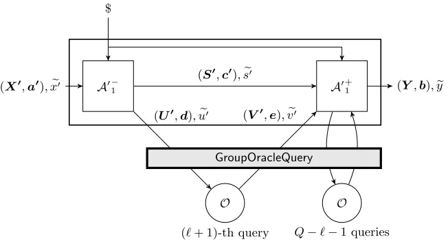
We show that |Succ`+1−Succ`| is negligible, under the conditions stated in the lemma. Indeed, we can splitAgen into two sectionsA−
` and A
+
` separated by the`-thGroupOracleQuery call, as shown in
Figure 3.
Observe that in either of the two scenarios, that is usingOhy`-genorOhy`+1-gen,A−
` is in itself a generic
oracle algorithm interacting withOpa-gen. Indeed, we can replace the bounded polynomial sourceD, the generic algoritm sectionA−` and the first `queries to GroupOracleQuery by another equivalent bounded polynomial source, D`, with parameters (t,r1, . . . ,r`) and polynomial map extracted from lemmas 6
and 7.14 This reduces the problem to the case `= 0, but forD0 =D`,A0
gen
=A+`,Q0 =Q−`,`0 = 0 and ([x0]a0,xe0) = [s]c,[v]e,ex,ev). However, the non-group elementsxe0 = (es,ev) in the input of A0
gen now could be correlated with its random tape. Notice that the case`=Q becomesQ0 = 0 which is again a particular case of Lemma 1. We focus now on` < Q (that is,A+ makes at least one GroupOracleQuery call).
We analyze the differences between the two games in whichA0gen
interacts with eitherOhy0-gen=Ogen
orOhy1-genforQ0≥1. We consider again the splitting ofA0geninto A0−
1 andA0 +
1, shown in Figure 4. In both games,A0+
1 is interacting withOgen. Hence, the only differences between the games can be produced byA0−
1 via a nontrivial GroupEqTest query, since A0−1 is making no GroupOracleQuery calls. According to Lemma 1, these nontrivial queries occur only with a negligible probability (even when the non-group
14
Actually, for fixed xe and the random tape, Lemma 6 gives polynomials S1, . . . , Sγ, V1, . . . , V ∈
(X,a),xe
$
A− `
O
`−1 queries
O
`-th query
O
Q−`queries
A+
` (Y,b),ye
(S,c),es
(U,d),eu (V,e),ve
GroupOracleQuery
Fig. 3.Splitting of the generic algorithm in Lemma 8, for 1≤`≤Q.
(X0,a0),xe0
$
A0− 1
O
(`+ 1)-th query
O
Q−`−1 queries
A0+
1 (Y,b),ey
(S0,c0),se0
(U0,d),ue0 (V
0
,e),ve0
GroupOracleQuery