Comparison of Numerical Simulations of the Electron Density in the D-Region Ionosphere with Measurements of the Radar of Partial Reflections

(1)

Comparison of Numerical Simulations of the Electron Density in

the D-Region Ionosphere with Measurements of the Radar of

Partial Reflections

Aleksandr Gomonov1,2,*, Roman Yurik1,2, Yulia Shapovalova1, Sergei Cherniakov,1 and Olga Ogloblina1

1

Polar Geophysical Institute, RU-183010

,

Murmansk, Russian

2

Murmansk Arctic State University, RU-183038, Murmansk, Russian Federation

Abstract. The paper reports results of a comparison of the measured electron density in the ionospheric D-region measured using the partial reflection facility at the observatory. Tumanny of the Polar Geophysical Institute (69.0°N, 35.7°E) with numerical simulations performed using the theoretical model of the Polar Geophysical Institute (PGI) (Murmansk, Russian Federation). The model was examined using experimental data obtained under quiet geomagnetic conditions in March, 2017. The comparative analysis carried out in this study shows a very good agreement of the PGI model with experimental data and indicates that the IRI-2016 model fails to adequately reproduce measurements in regions with high electron density gradients.

1 Introduction

The D–region of the ionosphere covers the altitude range of 50–90 km. The knowledge of its properties is very important as well as for applied interest and for scientific one. The D–region of the ionosphere has a significant influence on the radio waves propagation in the wide frequency bands. The D-region remains not enough studied region of the ionosphere for various reasons. The behavior of the D-region of the ionosphere is quite complicated even in calm conditions of mid-latitudes, and is quite difficult for experimental study because there are the low electron density, the complex composition of the ions and the high density of the neutral atmosphere. The behavior of the ionosphere at high latitudes is much more complex, as corpuscular sources of ionization are very often observed: mainly electrons in the auroral oval and solar protons in the polar region. It is very impotent to create mathematical, and then computer models of the D–region that can describe the behavior of the main ionospheric parameter - the electron density (Ne) - under various

heliogeophysical conditions.

The radar has been designed by the Polar Geophysical Institute (PGI) (Murmansk, Russian Federation) to study the lower ionosphere by the method of partial reflections [1-3] and have been used for investigation and comparisons with methods [4-5]. The medium frequency (MF) radar of vertical sounding of the ionosphere by the partial reflection method is the main effective instrument for the quantitative study of the lower ionosphere, which allows continuous observations for a long time. This radar is situated at the radio physical observatory Tumanny of the Polar

Geophysical Institute (69.0 N, 35.7 E) and is unique one. It has been working since 1991 on a regular basis.

2 Characteristics of the

medium

frequency radar of vertical sounding

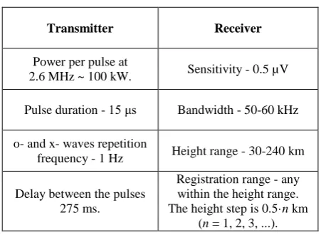
The characteristics of the medium frequency radar for vertical sounding of the ionosphere are represented in Table 1.

Table 1. Technical characteristic of the MF-radar.

Transmitter Receiver

Power per pulse at

2.6 MHz ~ 100 kW. Sensitivity - 0.5 µV Pulse duration - 15 μs Bandwidth - 50-60 kHz o- and x- waves repetition

frequency - 1 Hz Height range - 30-240 km

Delay between the pulses 275 ms.

Registration range - any within the heightrange. The height step is 0.5·n km

(n = 1, 2, 3, ...).

(2)

south-west to north-east. Therefore, the beam width is nonsymmetrical and it equal to 19° along the north-east direction and 30° along the north-west direction. The side lobe level is 12% [6].

Fig.1. The MF-radar antenna array layout.

3 Measurements

It is known that electron density in the D-region of the ionosphere can be obtained by calculations from the measured amplitudes of ordinary Ao(h) and

extraordinary Ax(h) waves partially reflected by the

ionospheric plasma in two ways: by the differential absorption method or by the correlation method.

These methods for determination plasma parameters are based on the emission of two wave modes in the form of alternating pulses. Separate receiving of the signals partially reflected by electron density irregularities and suggested frequency of collisions between electrons and neutral particles, as well as measured amplitudes in dependence on the time delay determined by the reflection height constitute this method [7, 8].

The distribution of electron density Ne(h) (Fig. 2) can

be determined from the measured ratio Ax(h)/Ao(h),

under certain conditions, using the equation:

) ( ) ( ) ( ln ) ( ln ) ( h K h A h A h R dh d h N o x               −

= , (1)

where K(h) = 2[kx(h)-ko(h)]/N, kx,o(h) - are the

absorption coefficients of the extraordinary (x) and ordinary (o) radio waves, determined by the operating frequency, the electron gyrofrequency and the altitude profile of the electron-molecule collisions frequency, R(h) = |Rx(h)|/|Ro(h)|, |Rx, o(h)| - are the absolute values

of reflection coefficients.

Measurements of the electron density of Ne in the D–

region of the ionosphere are both expensive and local in space. In this regard, a computer model of the ionization-recombination cycle of the D-region of the ionosphere was created at the Polar Geophysical Institute (Murmansk) [9].

Fig. 2. An example of measuring of the electron density Lg(Ne) (cm-3) 13 March 2017.

This model includes four positive ions NO+, O2+,

Cb1+, Cb2+ and four negative ions O2-, O-, CO3-, NO3

-and electrons [9]. The justification of the model, the constants of the velocities of processes in it are given in. The model takes into account the variations of Ne(h) due

to the zenith angle of the Sun, solar activity, and the seasons of the year. The profile Ne(h) in the model is

determined by the following analytical expression:

( ) 0 ( )

0

91 ( ) ( ) cos [1 ( ) cos( 360 )]

365

n h h R

kp

m

Ne h =N h c +k h − eα (2)

whereN h₀( ) - is the electron density profile corresponding to the day of the autumn (spring) equinox at the effective zenith angle of the sun

c

_kp= 0 and the

minimum solar activity R=0.

The exponent in formula (2), which determines the dependence of Ne(h) on the zenith angle of the Sun, is

represented by the function:

0

( ) _ncos( n 360 )

n

B h

n h A

C

−

= (3)

with coefficientsA_n=0, 9,

B

_n

=

80, 0

, C_n=131, 2.

This gives a maximum dependence of Ne(h) on

c

_kp

at 80 km _cos0,9

kp

c and a minimum _cos0,5

kp

c at the height of 50 km.

The corrected (effective) zenith angle of the sun had been used in order to take into account asymmetry of daily variations _{( )} ₍ _{0, 5)}

kp t t

c =c − , where t - local time in hours.

The dependence of the electron density on solar activity (the number of sunspots R) is given by the ratio:

_Ne

_~

_e

α( )h R₍₄₎ The proportionality coefficient α(h) (determined only from rocket data) is approximated by the expression:

( )h A (1 C ) h B α α α α = − − (5)

(3)

Electron density decreases when increasing solar activity at the height of 60 km and grows in the heights range of 62-90 km in accordance with (5). The growth of Ne(h) becomes sharper with increasing of height. The

electron density Ne(h) increases in 1.9 times at the height

of 70 km and 2.9 times at the height of 90 km when passing from a minimum (R = 0) to a maximum of solar activity.

It had been shown earlier [9] that this model allows to reliably describe seasonal variations of the ionic composition and electron density, which are reliably established from rocket data, as well as the winter anomaly of the region D.

The calculation of the model (PGI) provides the scientists and researchers with a number of options that allow solving various problems. This model is the most suitable for estimation of the electron density in the D -region in the Arctic -region.

Comparison analysis between of experimental data of measurements with the model calculations was carried out for selected dates under quiet geomagnetic conditions (March 13, 14, 16-20, 24-26, 2017) (Fig. 3, 4).

Fig. 3. F10.7 index (solar radiation flux at the wavelength of

10.7 cm, in units ×1022 W/(m2·Hz).

Fig. 4. Ap-index.

As it can be seen from the diagram in Fig. 3, during the period from March 13 to March 26, the flux of solar radio emission at the wavelength of 10.7 cm (index F10.7,

left panel) varied slightly, within 68.8-76.8 (in units of 1022 W/(m2·Hz)). For this period, the Ap-index in Fig.4

ranged from 1 to 24, which corresponds to the Kp values

from 0+ to 4-.

The measurement data of Ne(h) were compared with

the simulation results on selected days. The coordinates of the partial reflection radar were set in the (PGI) model. The data of solar activity parameters were fed to the model input. The averaged measurement data were compared with the model averaged data.

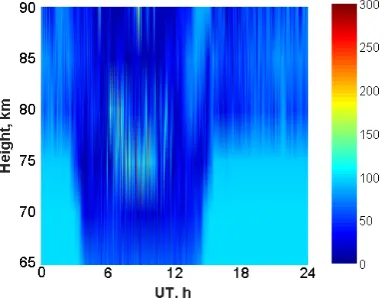
Fig. 5. The average electron density of model data (lg[Ne],

cm3) on March 13, 14, 16-20, 24-26, 2017.

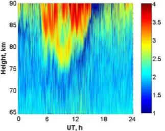
In the Fig.5 diurnal variations of electron density profiles are shown in the altitudinal range from 65 to 90 km according to model calculations and observations in Fig.6.

Fig. 6. The averaged electron density of experimental data (lg[Ne], cm-3) on March 13, 14, 16-20, 24-26, 2017.

The ten-days averaged electron density profiles Ne(h) were constructed from the model and observations data at the four moments: 02:00 UT, 10:00 UT, 12:00 UT, and 22:00 UT and are shown in Fig. 7 (red lines correspond to the calculations by model (PGI) and blue lines correspond to the profiles calculated from measurements).

(4)

profiles of Ne(h) on days with a quiet geomagnetic

situation for different times of the day.

Fig. 7. Electron density (lg[Ne], cm-3).

4 Conclusions

The algorithm for calculating of the electron density which was presented in this article and the computer model (PGI) was created on its basis are based on modern concepts of the ionization-recombination cycle in the lower ionosphere. The model takes into account all the main sources of ionization in the D-region of the ionosphere under quiet geomagnetic conditions . The ion-molecular reactions are included in the model make it possible to describe the influence of a neutral atmosphere, its daily and seasonal variations on ionospheric parameters (electron density). The model allows to take into account the heights variations of electron density, its seasonal changes for quiet geomagnetic conditions.

The calculation of the relative errors of measurements of the electron density of Ne(h) with

model data is shown in (Fig. 8).

Fig. 8. The calculated relative errors of Ne(h) determination.

Relative errors were calculated as a ratio between module of difference experiment data and model data of electron density to the module of experiment data of

electron density. Then the obtained result was multiplyed on 100.

The standard deviation of the measurement data of electron density is represented in Fig. 9.

Fig. 9. The standard deviation of the measurement data of electron density.

As we can see in Fig. 9 the standard deviation of the measurement data of electron density for days for quiet geomagnetic conditions have not essential variations except for measurements on high heights in day time. This fact is obvious.

As can be seen (Fig. 8), the (PGI) model can be considered as adequate one, and the results of its simulation Ne(h) for the D-region of the ionosphere are

consistent with the measurement data. This can be explained by the fact that the (PGI) model of electron density was specially developed for the Arctic region, and its parameters were selected for the conditions of the high latitudes. On the contrary of the (PGI) model, the IRI-2016 model, should be adjusted in the areas with high gradients of electron density Ne(h) [10].

References

1. V.A. Tereshchenko, V.D. Tereshchenko, S.M. Chernyakov, Proc. MSTU 13(4/2), 1052-1059 (2010)

2. S.M. Chernyakov, V.A. Tereshchenko, O.F.

Ogloblina, E.B. Vasiliev, A.D. Gomonov, Izv. vuzov. Fizika 12(2), 50-53 (Rus) (2016)

3. A.D. Gomonov, R.Yu. Yurik, Yu.A. Shapovalova, In. Science and Education in the Arctic Region 150-155 (2018)

4. M. Klimenko, V. Klimenko, I. Despirak, I. Zakharenkova, B. Kozelov, S. Cherniakov, E. Andreeva, E. Tereshchenko, A. Vesnin, N. Korenkova, A. Gomonov, E. Vasiliev, K. Ratovsky, Journal of Atmospheric and Solar-Terrestrial Physics 180, 78-92 (2018)

(5)

6. V.D. Tereshchenko, E.B. Vasiliev, N.A. Ovchinnikov, A.A. Popov, Technique and methods of geophysical experiments (KSC RAS, Apatity, 2003).

7. Ya.L. Alpert, Propagation of electromagnetic waves and the ionosphere (Nauka, Moscow, 1972).

8. J.A. Ratcliffe, An introduction to the physics of the ionosphere and magnetosphere (Cambridge University Press, Cambridge, 1972).

9. N.V. Smirnova, Modeling of the ionization-recombination cycle of the D-region, in Mathematical modeling of complex processes (USSR Academy of Sciences, Apatity, 1982).