Effect of Rotation on Rayleigh-Bénard- Marangoni Convection in a Relatively Hotter or Cooler Layer of Liquid

Effect of Rotation on Rayleigh-Bénard-

Marangoni Convection in a Relatively Hotter

or Cooler Layer of Liquid

A.K. Gupta

1

_{, S.K. Dhiman}

2

Professor, Department of Mathematics, Himachal Pradesh University Centre for evening studies, Shimla, India1

Assistant Professor, Department of Mathematics, Government Post Graduate College, Dharamshala, India2

ABSRACT: The effect of uniform rotation on the onset of steady Rayleigh-Bénard- Marangoni convection in a relatively hotter or cooler layer of liquid is studied theoretically by means of modified linear stability theory and a normal mode analysis. The top surface of layer is non-deformable free where surface tension gradients arise on account of variation of temperature, and the bottom surface is rigid and thermally conducting. Both mechanisms causing instability namely, surface tension induced and buoyancy induced are taken into consideration. A Fourier series method is used to obtain the eigenvalue equation analytically which is then computed numerically. Numerical results obtained are found to be significant from both qualitative and quantitative points of view. It is shown that uniform rotation in a relatively hotter layer of liquid is relatively more stable than a cooler layer of the same liquid under identical conditions. When speed of rotation becomes sufficiently large, it is found that the two mechanisms causing instability become less tight as compared to the case when no rotation is present. The asymptotic behavior of the rotation for the large values of the Taylor number is also obtained.

KEYWORDS: Buoyancy, Convection, Linear stability, Surface tension, Taylor number

I. INTRODUCTION

The mechanism of the onset of surface tension induced convection in a thin horizontal fluid layer heated from below with free upper surface was first reported experimentally by Block [5] and explained mathematically by Pearson [13]. They established that the patterned hexagonal cells observed by Bénard [3, 4] and explained by Rayleigh [14] in terms of buoyancy, were in fact due to temperature dependent surface tension. Convection driven by surface tension gradients is now commonly known as Bénard-Marangoni convection in contrast to the buoyancy driven Rayleigh-Bénard convection. Quantitative disagreement between experiment and theory has indicated that gravity was present in Bénard's experiments as well as in other experiments involving convection in a fluid layer with free surface in a laboratory on the earth, therefore, Nield [11] considered the combined effects of both the surface tension and buoyancy on the onset of convection in a liquid layer heated from below with free upper surface, called Rayleigh-Bénard-Marangoni convection, and found that the two effects causing instability are tightly coupled. For a detail study of convection one may be referred to the work of Chandrasekhar [6], Normand et al. [12] and Koschmieder [9].

II. RELATED WORK

actual decrease in its specific heat at constant volume, must exhibit convection at a higher temperature difference, hence more stable, than a cooler layer of the same liquid under identical conditions otherwise.

In the present investigation, we wish to study the influence of rotation on the onset of Rayleigh-Bénard-Marangoni convection in a relatively hotter or cooler layer of liquid being important in controlling and understanding qualitatively the mechanism of convective instability problems encountered in geophysics, oceanography, atmospheric sciences and chemical engineering of paints and detergents. This analysis extends the work of Gupta et al. [7] to include the effect of Coriolis force. The Fourier series method is used to obtain the eigenvalue equation analytically. The numerical results are obtained for a wide range of parameters relevant to the problem in the present context. The results of this analysis indicate that the critical eigenvalues in the presence of Coriolis force are greater in a relatively hotter layer of liquid than a cooler one under identical conditions otherwise. The vital role that a relatively hotter layer of liquid has stabilizing influence in the presence of rotation as compared to that which is relatively cooler under almost identical conditions is illustrated through neutral stability curves. In addition, we find that when speed of rotation becomes sufficiently large, the two mechanisms causing instability become less tight as compared to the case when there is no rotation present. The asymptotic behavior of the rotation for large values of Taylor number is also obtained and discussed.

III. MATHEMATICAL FORMULATION OF THE PROBLEM

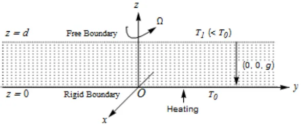
The physical configuration of the problem consists of an infinite horizontal layer of viscous fluid of uniform thickness d heated from below and which is kept rotating with a constant angular velocity Ω about an axis parallel to the direction of gravity. The lower rigid boundary of the layer maintained at constant temperature T0 and the upper free

surface is open to the atmosphere at temperature T1 (<T0) subject to general heat radiative condition. We choose a

Cartesian coordinate system Oxyz so that Oz coincides with the axis of rotation and Ox and Oy lie in the plane of the

lower surface of the layer so that the fluid layer is confined between the planes atz = 0 and z = d. The surface tension on

the upper free surface of fluid layer is regarded as a function of temperature only which is given by the simple linear law





1 T T1

  

   (1)

where the constant ₁ is the unperturbed value of  at the unperturbed surface temperature TT₁ and





1

/ T T T

  _

    represents the rate of change of surface tension with temperature, evaluated at temperature T₁, and

surface tension being a monotonically decreasing function of temperature,  is positive.

FIGURE 1. Schematic representation of the physical configuration of the problem

2 2 2

1 2 ,

v w g

t z



 

 

 _{  } _{   }

_  _

  (2)

2 2 0

(1 T) w,

t













 _   _  

  (3)

2

2 w,

t





z

 

 _{ }  _{ }

_  _

  (4)

wherew is the perturbation velocity,  the perturbation temperature,



is the z-component of vorticity. The adverse

uniform temperature gradient







T0T1



/d0 , the gravitational acceleration g, the coefficient of volume

expansion , the kinematic viscosity v, the thermal diffusivity  are each assumed constant, 2 and ₁2 represent respectively

2 2 2 2 2 2

x y z

  

 

   and

2 2 2 2

x y

 



  ,

andt represents time. Further, the coefficient ₂ (due to variation in specific heat at constant volume on account of

variations in temperature) lies in the range from 0 to 104 and that range of the dimensionless parameter _{2 0}T covering

the usual laboratory conditions is 0_{2 0}T 1 for liquids with which we are mostly concerned. In this range, any

given value of



_{2 0}T

 

0 corresponds to the layer of liquid which is relatively hotter compared to that associated with

its value(including _{2 0}T 0) less than the given one. A detailed account of this has been given in the research monograph by Banerjee and Gupta [1].

Equations (2) – (4), must be solved subject to appropriate boundary conditions. For the rigid and perfectly thermally

conducting (the perturbation temperature is thus zero) lower boundary at z = 0, the boundary conditions are

0, w 0, 0, 0.

w

z  



   

 (5a,b,c, d)

Since the tangential viscous stress experienced by the liquid at the upper free surface is balanced by the traction due to

variation with temperature of surface tension, and the general heat radiation condition at z = d, the boundary conditions

are

2

2 1 2

0, w , , 0,

w k q

z z

z









 







     

 

 (6a,b,c, d)

wherek is the heat conductivity and q is the rate of change with temperature of the time rate of heat loss per unit area

from the upper surface.

We now analyze an arbitrary disturbance in terms of normal modes assuming that the perturbations w,



and



are of

the form



, , , ,

 

, , , ,

 

, , ,



     

, , Z exp





_{x y}





w x y z t



x y z t



x y z t  W z  z z i a x a y st

   

   

wherea_x and ay are components of the horizontal wave number





2 2

x y

a  a a of the disturbance, and s is the time

growth rate (a complex number in general). Using the above expressions for w, and



in equations (2) – (4) and

then making the resulting equations dimensionless by choosing d d, 2/ ,v



/ d,



d v k



/



as units of length, time, velocity and temperature scales respectively, we obtain



 



1

2 2 2 2 2 2 _,

D a D a p W RaT DZ (7)







2 2







2 0 2 0

1 _r 1 ,





1

2 2 2 _.

D a p Z  T DW (9)

HereR



gd4/



is the Rayleigh Number, P_r





 

/



is the Prandtl Number, T



 4 2d4 2



is the Taylor Number.

We restrict our analysis to the case when the principle of exchange of stabilities is valid for the present problem

so that instability first sets in as stationary convection. In that case, the marginal state is characterized by p= 0, and

equations (7) – (9) reduces to





1

2

2 2 2 2 _,

D a WRaT DZ (10)



2 2







2 0

1 ,

D a    T W (11)





1

2 2 2 _.

D a Z  T DW (12)

In terms of new variables, the non-dimensional form of boundary conditions (5a, b, c, d) – (6a, b, c, d) can be written as

 

0 0,

 

0 0

W  DW  , 

 

0 0, Z(0) = 0, (13a, b, c, d)

evaluated on the lower boundary z = 0, and

 

2

 

2

 

 

 

1 0, 1 1 0, 1 1 0, (1) 0.

W  D W a M  D  L  DZ  (14a, b, c, d)

evaluated on the upper boundary z = 1. Here M 



d2/



v is the Marangoni number and Lqd k/ is the Biot number.

Equations (10) – (12) together with boundary conditions (13a, b, c, d) – (14a, b, c, d) constitute an eigenvalue problem

of order eight with M as an eigenvalue for given values of the remaining parameters.

IV. SOLUTION OF THE PROBLEM

The Fourier series method as presented by Nield [11] is convenient for the problem under consideration. We let

 



2

   

2

 



3 3 1

2

0 1n 1 sin ,

n n

W z A D W D W n z

n





     _    _  



(15)

 

 

 

1 2

1n 1 sin ,

n n

z B n z

n









 

  _    _

 



(16)

0 2 2 1

2 1

( ) (0) cos (0),

3

n n

Z z C C DZ n z DZ

n





      _  _   



(17)

where the boundary conditions (13a, c) and (14a, d) have already been used while writing equations (15)-(17). The differential equations (10)-(12) are satisfied by substituting W(Z), (z), Z(z) and their derivatives, we obtain the system of equations which can be solved for A Bn, nandCn. Substitution of A Bn, nandCnin the remaining boundary conditions we get three linear homogeneous algebraic equations. Finally, elimination of the unknown constants

2

(0), (1) and (1)

DW D W DZ yields the eigenvalue equation as

 

 

 

 









 









_

_

 

1 1 1 1

2 2 2 2 2 2

1 1 1 1

2 2 2 2

1 1 1 2 0 1 2 0 1

1 1

1 1

1 1 1 1 1

2 1

1

n n

n n

n n

n n n n n n n n

n n

n n

n n

n n n n n n n n

n n

n n n n n

n n n n n n n n n n

F E

F E

M R

H H H H

E E

E E

M R H

H H n a H n a H

E E L G E E

M R

H H H a T H T n a H

                                         _{ }   _ _    _    



























T T T _T



2 2 2



1

0

n n a Hn

where

















2 2 2 2 2 2 2

2 2 2 2 2

3

2 2 2 2 2 2 2 0 1 1 coth 2 n n n n E n

F n n a

G a n a

H n a a R T n

H a a                         _     T (19)

We can obtain M from the eigenvalue equation (18) in terms of a, R, L, Q and_{2 0}T as the ratio of two determinants

given by

 

















_

_

_

 

_

1 1 1

2 2 2 2 2 2

1 1 1

2 2 2 2 2 2 2

1 1 2 0 1 2 0 1 1

1

( 1)

1

1

( 1) 1 1 1

2 1

1

( 1)

n

n n n

n n n n n n

n n

n n

n n n n n n

n n

n

n n n

n n n n n n n n n n

n

n n

n n

F E E

R

H H H

E

E E

R H

H n a H n a H

E

E L G E

R

H H a T H T n a H n a H

M F F H                                          _{ }  _{ }   _       

























T T T _T





 





1 1

2 2 2

1 1 1

2 2 2

1 1 1

, (20)

( 1)

1 ( 1)

n

n n n n

n

n n n

n n n n n n

n n

n

n n

n n n n n n

E

H H

E E E

H

H H n a H

E

E E

H H n a H

                   _    

















T T T

V. NUMERICAL RESULTS AND DISCUSSION

The numerical calculations may be carried out as follows. For fixed values of T , _{2 0}T and L the expression (20) determines the Marangoni number M as a function of the wave number a. The minimum value of M is the critical

Marangoni number Mc and the value of a at which M attains the minimum is the critical wave number aM .

Alternatively, for fixed values of M,T ,_{2 0}T and L, we may determine the Rayleigh number R as a function of the

wave number a. The minimum value of R is the critical Rayleigh number Rc and the value of a at which R attains the

minimum is the critical wave number a_R. By either means we can plot the (R, M)-curve for fixed values of T , _{2 0}T

and L corresponding to the marginal stability.

According to the procedure as described above, numerical values are computed with the aid of symbolic algebraic

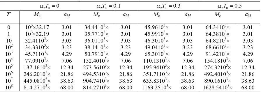
package Mathematica 5.2. The numerical values of Mc and aM (R = 0) computed from expression (20) when L = 0 and

3 10

L are respectively presented in Table 1 and Table 2 for fixed values of _{2 0}T andT _{. The values of} T are chosen

so as to compare the results obtained by us with the results of Namikawa et al. [10]. We find that when _{2 0}T 0

by Namikawa et al. [10]. When T = 0 the results obtained here for various values of _{2 0}T agree precisely with corresponding values obtained by Gupta et al. [7].

TABLE 1. Values of Mcand aM for various values of 2 0T when L = 0

2 0T 0

  _{2 0}T 0.1 2 0T 0.3 2 0T 0.5

T Mc aM Mc aM Mc aM Mc aM

0 79.61 1.99 88.45 1.99 113.72 1.99 159.21 1.99

1 79.73 2.00 88.59 2.00 113.90 2.00 159.47 2.00

10 80.86 2.01 89.84 2.01 115.51 2.01 161.72 2.01

102 91.35 2.17 101.50 2.17 130.51 2.17 182.71 2.17

103 163.41 2.97 181.56 2.97 233.44 2.97 326.81 2.97

104 456.92 5.01 507.69 5.01 652.75 5.01 913.85 5.01

105 1401.76 8.63 1557.51 8.63 2002.51 8.63 2803.52 8.63

106 4405.48 15.11 4894.98 15.11 6293.54 15.11 8810.96 15.11

107 13925.70 26.80 15473.00 26.80 19893.86 26.80 27851.40 26.80

108 44036.70 47.65 48929.67 47.65 62909.57 47.65 88073.40 47.65

TABLE 2. Values of Mcand aM for various values of 2 0T when L = 10

3

2 0T 0

  _{2 0}T 0.1 2 0T 0.3 2 0T 0.5

T Mc aM Mc aM Mc aM Mc aM

0 103×32.17 3.01 34.44103× 3.01 45.96103× 3.01 64.34103× 3.01

1 103×32.19 3.01 35.77103× 3.01 45.99103× 3.01 64.38103× 3.01

10 32.41103× 3.03 36.01103× 3.03 46.30103× 3.03 64.82103× 3.03

102 34.33103× 3.23 38.14103× 3.23 49.04103× 3.23 68.66103× 3.23

103 45.71103× 4.29 50.79103× 4.29 65.30103× 4.29 91.42103× 4.29

104 77.09103× 7.06 152.40103× 7.06 110.13103× 7.06 154.18103× 7.06

105 137.16103× 12.34 273.56103× 12.34 195.94103× 12.34 274.32103× 12.34

106 246.20103× 21.86 494.53103× 21.86 351.71103× 21.86 492.40103× 21.86

107 445.08103× 38.63 904.74103× 38.63 635.83103× 38.63 890.16103× 38.63

108 814.27103× 68.00 814.27103× 68.00 1163.25103× 68.00 1628.54103× 68.00

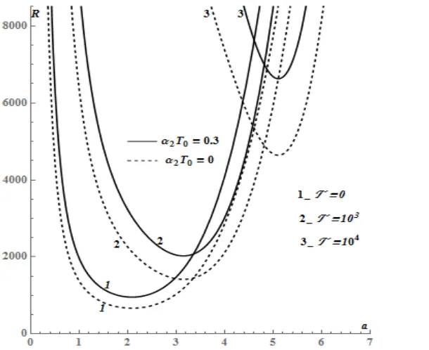
The neutral stability curves for the limiting cases namely, Bénard-Marangoni convection (R= 0) and for

Rayleigh-Bénard convection (M=0) are plotted respectively in Fig. 2 and Fig. 3 for various values of T and _{2 0}T when L = 0.

FIGURE 2. Bénard-Marangoni neutral stability curves for various values of T and _{2 0}T when L = 0.

FIGURE 3. Rayleigh-Bénard neutral stability curves for various values of T and _{2 0}T when L0

The upward moving neutral stability curves in Fig 2 and 3, illustrate that increasing values of either the Taylor number

layer of liquid is relatively more stable in the presence of rotation compared to a relatively cooler one under almost identical conditions in each case.

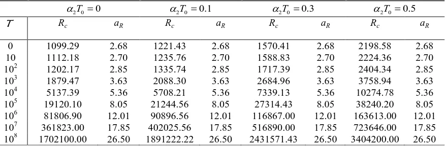
The numerical values of both Rc and aR(M = 0) computed from expression (18) when L = 0 and

3 10

L are

respectively presented in Table 3 and Table 4 for various given values of _{2 0}T andT . When _{2 0}T 0 values of Rc and

R

a for various values of T obtained here agree precisely with corresponding values as obtained by Namikawa et al. [10].

For fixed values of _{2 0}T and T , it may be mentioned here that as L increases values of both Mc and Rc increase. In the

limit L, we find that value of Mc becomes asymptotically proportional to L while that of Rc tends to a finite limit.

In either case, the corresponding critical wave number remains finite. The case when L increases from 0 to 

corresponds to the situation wherein thermal boundary conditions at the free surface changes from constant heat flux

 



D 1 0



to constant temperature





 

1 0



. Therefore, when L is small it is easier for temperature perturbations

to be set-up, but when L is large, any temperature variations across the free surface decay rapidly. Thus as L becomes

large, the values of Mc tend to infinity since it becomes difficult for the surface tension to be operative, while those of

Rc remain finite since the buoyancy force is still operative.

TABLE 3. Values of Rcand aR for various values of 2 0T when L = 0

2 0T 0

  _{2 0}T 0.1 2 0T 0.3 2 0T 0.5

T Rc aR Rc aR Rc aR Rc aR

0 669.00 2.09 743.33 2.09 955.71 2.09 1337.99 2.09

10 679.70 2.11 755.22 2.11 971.00 2.11 1359.39 2.11

102 769.87 2.28 855.41 2.28 1099.81 2.28 1539.74 2.28

103 1418.95 3.15 1576.61 3.15 2027.07 3.15 2837.90 3.15

104 4640.20 5.11 5155.78 5.11 6628.86 5.11 9280.40 5.11

105 18695.70 7.94 20773.00 7.94 26708.14 7.94 37391.40 7.94

106 81478.40 11.96 90531.56 11.96 116397.71 11.96 162956.80 11.96

107 369697.00 17.83 410774.44 17.83 528138.57 17.83 739394.00 17.83

108 1711750.00 26.49 1901944.44 26.49 2445357.14 26.49 3423500.00 26.49

TABLE 4. Values of Rcand aR for various values of 2 0T when L = 10

3

2 0T 0

  _{2 0}T 0.1 2 0T 0.3 2 0T 0.5

T Rc aR Rc aR Rc aR Rc aR

0 1099.29 2.68 1221.43 2.68 1570.41 2.68 2198.58 2.68

10 1112.18 2.70 1235.76 2.70 1588.83 2.70 2224.36 2.70

102 1202.17 2.85 1335.74 2.85 1717.39 2.85 2404.34 2.85

103 1879.47 3.63 2088.30 3.63 2684.96 3.63 3758.94 3.63

104 5137.39 5.36 5708.21 5.36 7339.13 5.36 10274.78 5.36

105 19120.10 8.05 21244.56 8.05 27314.43 8.05 38240.20 8.05

106 81806.90 12.01 90896.56 12.01 116867.00 12.01 163613.00 12.01

107 361823.00 17.85 402025.56 17.85 516890.00 17.85 723646.00 17.85

108 1702100.00 26.50 1891222.22 26.50 2431571.43 26.50 3404200.00 26.50

The asymptotic behavior of Mc as Q depends critically on both 2 0T and L, whereas the asymptotic behavior of

M

2 0 4.40 1

c M

T  

 T

1

2_{and 0.48}

M

a  T

1 4

Which are in close agreement with the values M_c  4.42T

1

2_{and 0.5}

M

a  T

1

4_{as obtained by Vidal and Acrivos [15]}

(when _{2 0}T 0) by means of asymptotic analysis.

When L= 103, we obtain

2 0 0.81 1

c M

L  T T

1

2_{and 0.69}

M

a  T

1 4

On the other hand, the asymptotic behaviour of Rc and aR as T   is independent of L. However, the asymptotic behavior of Rc critically depends on α2T0. In this case, we find that

2 0 7.95 1

c R

T  

 T andaR 1.23T

1 6

which are in close agreement with the values R_c≈8.69T

2 3 _and

R

a ≈1.31T

1

6 _{as obtained by Vidal and Acrivos [15]}

(when α2T0= 0).

The (R, M)-loci corresponding to neutral stability curves for the combined surface tension and buoyancy effects, normalized for critical values of Rc and Mc are plotted in Fig 4 for various values of T and 2 0T for the limiting case

when L=0 (insulating boundary).

FIGURE 4. (R, M)- loci corresponding to Rayleigh-Bénard-Marangoni neutral stability curves (normalized to give unit

intercepts) for various values of T and _{2 0}T when L= 0.

Fig. 4 shows that the inhibiting effect of the Coriolis force remains unchanged. Comparison of curves in Fig. 4 illustrate

that when T = 0 the coupling between the two agencies remain tight but not perfect. If there were perfect coupling, one

line R R/ _cM M/ _c1/ (1_{2 0}T),illustrating that the coupling between the two mechanism causing instability becomes less tight.

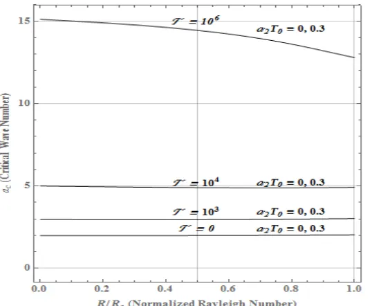
FIGURE 5.Wave number corresponding to Rayleigh-Bénard-Marangoni neutral stability versus normalized Rayleigh number.

Fig. 5 illustrate the variation of wave numbers corresponding to the Rayleigh-Bénard-Marangoni at the marginal

stability. For large values of T the convective cells increase in size, independent of _{2 0}T , at the onset of convection as

the dominance of buoyancy effect increases.

VI. CONCLUSION

The modified linear stability analysis of the Rayleigh-Bénard-Marangoni convection in a relatively hotter or cooler layer of liquid in the presence of rotation has been studied theoretically and we conclude that Coriolis force is relatively more stabilizing in a relatively hotter layer of liquid than a cooler one under identical conditions, irrespective of whether the driving force is either surface tension or buoyancy or both surface tension and buoyancy.

Acknowledgement: We are grateful to Professor R.G. Shandil (Retd.), Department of Mathematics, H.P. University, Shimla-171005, for his valuable advice during the course of present work.

REFERENCES

[1] Banerjee M.B. and Gupta J.R., “Studies in Hydrodynamic and Hydromagnetic Stability”, Silver Line Publication, Shimla, 1991. [2] Banerjee M.B., Gupta J.R., Shandil R.G., Sharma K.C. and Katoch D.C., “A modified analysis of thermal and thermohaline instability of

a liquid layer heated underside”, J. Math. Phys. Sci., Vol. 17, pp.603-629, 1983.

[3] Bénard H., “Les tourbillons cellulairesdansunenappeliquidetransportant de la chaleur par convection en regime permanen”, Revuegenerale des Sciences pures at appliqués, Vol. 11, pp.1261-1271, 1900.

[4] Bénard H., “Les tourbillons cellulairesdansunenappleliquidetransportant de la chaleur par convection en re’gime permanent”, Ann. Chimie (Paris), Vol. 23, pp.62-144, 1901.

[5] Block M.J., “Surface tension as the cause of Bénard cells and surface deformation in a liquid film”. Nature, Vol. 178, pp.650-651, 1956. [6] Chandrasekhar S., “Hydrodynamic and Hydromagnetic Stability”, Dover Publications, New York, 1961.

[8] Hashim I. and Sarma W., “On the onset of Marangoni convection in a rotating fluid layer”, J. Phy. Soc. Japan, Vol. 75(3), pp. 035001-2, 2006.

[9] E.L. Koschmieder, “Bénard Cells and Taylor Vortices”, Cambridge University Press, Cambridge, 1993.

[10] Namikawa T., Takashima M. and Matsushita S., “The effect of rotation on convective instability induced by surface tension and buoyancy”, J. Phy. Soc. Japan, Vol. 28 (5), pp. 1340-1349, 1970.

[11] Nield D.A., “Surface tension and buoyancy effects in cellular convection”, J. Fluid Mech., Vol. 19, pp.341-352, 1964.

[12] Normand C., Pomeau Y. and Velarde M.G., “Convective instability: A physicist’s approach”, Rev. Mod. Phys., Vol. 49, pp.581-624, 1977.

[13] Pearson J.R.A., “On convection cells induced by surface tension”, J. Fluid Mech., Vol. 4, pp.489-500, 1958.

[14] Rayleigh L., “On convection currents in a horizontal layer of fluid, when the higher temperature is on the underside”, Phil. Mag., Vol. 32, pp.529-546, 1916.