Quantum mechanics and electromagnetism.
Non-relativistic theory.
Ladislaus Alexander B´
anyai* and Mircea Bundaru**
May 4, 2020
Institut f¨ur Theoretische Physik, Goethe-Universit¨at, Frankfurt am Main* banyai@itp.uni-frankfurt.de,corresponding author
National Institute of Physics and Nuclear Engineering - Horia Hulubei, Bucharest** bundaru@theory.nipne.ro
Abstract
We describe here the coherent formulation of electromagnetism in the nonrelativistic quantum-mechanical many-body theory. We use the mathematical frame of the field theory and its quantization in the spirit of the QED. This is necessary because of the manifold of misinterpretations emerging from the hystorical development of quantum mechanics, starting from the Schr¨odinger equation of a single particle in the presence of given electromagnetic fields, followed by the many-body theories of many charged identical particles having just Coulomb interactions inspired from the classical electromagnetic theory of point-like charges. However, this later is known to be inconsistent due to the self-interaction. This way could not be continued further to include properly the magnetic forces between the charged particles and lead to a lot of confusion about the interpretation of the magnetic field in the Hamiltonian, as well as about the gauge invariance. We emphasize the importance of the distinction between the applied (external fields) and the field in the matter. All these problems are length properly solved within the non-relativistic QED, nevertheless the confusion dominates in all the problems related to the magnetic properties of the solid state.
keywords: nonrelativistic QED, many-body theories, Lagrangian, gauge invariance, Coulomb gauge, Hamiltonian, external fields, quantization, 1/c2 approximation, current-current interaction
1
Introduction
The quantum mechanics of a single charged particle in the presence of applied electric and magnetic fields is based on the classical mechanics of a point-like charge derived from a Lagrange function, followed by a quantization by the prescription of the ”Poisson-bracket to commutator” recipe. This scheme was thereafter followed also in the description of the electromagnetic interaction between the charged particles. However, the classical electromagnetic theory of point-like charges has neither a Lagrangian nor Hamiltonian formulation. One eliminates by hand from the Lorentz force the action of the fields created by the particle itself. Nevertheless, one took over this recipe in order to include at least the Coulomb interaction between the particles. The constructed Hamiltonian lead to big successes as well in the theory of atomic structure, as in the solid-state theory. Of course, one had to include also the symmetry or antisymmetry of the wave functions due to the bosonic, or fermionic nature of identical particles, as well as the spin, whose origin stems actually from the relativistic theory. This state of the solid-state theory theory however was unable to include the magnetic field and forces created by the charged particles themselves. The importance of this problem was waved out by an argument relying on the small velocities of the electrons and ions in matter as to be compared to the light velocityc. This argumentation is nevertheless false, since it is well-known that a slow flow of a macroscopic number of electrons may create enormous magnetic fields. A first attempt to construct a Lagrangian and Hamiltonian including velocity-dependent forces up to 1/c2 in the classical theory of interacting charged point-like particles
was made by Darwin Ref.[1] almost 100 years ago. His idea was to neglect the retardation from the Lenart-Wichert potentials in order to eliminate them in favor of the particle velocities and ignoring the terms containing the velocity of the same particle. Only later Landau and Lifshitz Ref. [2] realized, that
one may not pursue this way without fixing the gauge. They have shown, that the Darwin Hamiltonian of order 1/c2 may be justified only in a very strange non-linear gauge. This would imply consequently a
constraint on the velocities. Nevertheless, this line of thought was continued up to these date in several publications even with some attempts to include it in the quantum-mechanical many-body theory.
This is a very strange situation, since already in the mid 20th century Quantum Electrodynamics (QED) was successfully developed, which is considered as the basic theory for the relativistic, quantum mechanical description of charged particles together with the electromagnetic field. Therefore, any non-relativistic quantum-mechanical description has to be derived as an approximation of the QED. In other words, the non-relativistic quantum mechanics of charged particles has to be reformulated accordingly without any reference to the ill-defined classical theory of point-like charges.
The relativistic QED of electrons and positrons coupled to photons is the basic pattern, but it is too far away to start with it. The quantum mechanical theory of the solid state operates only with electrons and ions as basic particles and actually after further approximations with Bloch electrons and phonons, or with electrons and holes in the conduction respectively valence bands within the effective mass approximation or even more simplified with electrons in a homogeneous positive background. These basically non-relativistic many-body theories of solid state, although had to include elements of the relativistic QED, like the spin degree of freedom with its magnetic moment, continued to work only with Coulomb interactions between these constituents inspired from the classical electrodynamics of point-like charges. This concept introduced a lot of confusion in the treatment of the magnetic phenomena. Within this frame was not possible to discern between internal and external magnetic fields. The magnetic field remained a mysterious object even in the treatment of superconductivity, where obviously only the magnetic field created by the electrons may explain perfect diamagnetism. The unique magnetic field used in today’s condensed matter theories has to be interpreted either as a self-consistent one (average of the total field), or as the external one. In the first case the choice of the gauge is already fixed in the Hamiltonian and in the second case there is a gauge freedom in the Hamiltonian, but this magnetic field remains unaffected by the presence of the matter.
Already in the classical macroscopic formulation of electromagnetism one is confronted with the dif-ference between the external (applied ) field, identical with the one in the absence of matter, and the true field in the presence of matter. This is valid, whether one speaks about longitudinal fields, or trans-verse ones. The quantum mechanics describing the interaction of matter with an external longitudinal electric fields was length properly treated. The same is true about the interaction with electromagnetic waves in the discussion of optical properties. Only the handling of the magnetic properties (leaving aside spin-magnetism) remained confuse, since no velocity dependent forces were taken into account. (See however the 50 years old book of Zubarev [3], where he already insisted on the importance of the general distinction between external and total fields in the frame of the linear response.)
Recently, one of these authors Ref. [4] has derived the correct 1/c2 interaction terms responsible for magnetic forces in a purely non-relativistic electron theory. His proof is based both on its derivation from the non-relativistic QED, as well as by an appropriate construction along the lines of Darwin [1] and Landau-Lifshitz [2], however in the Coulomb gauge containing only the physical degrees of freedom of the fields. Both lines lead to the same result. These results were actually contained implicitly in an old paper of Holstein, Norton and Pincus [5].
We describe here first the classical field theory of electromagnetic fields interacting with a Schr¨odinger electron. This approach is analogous to the starting point of the relativistic QED, which is based on the Dirac equation. The next step is the construction of the Lagrangian, which is not uniquely defined. There are two different ways to introduce the external fields or sources.
The first considers the ”internal” e.m. fields produced by the electron that interacts also with ”exter-nal” fields (produced by external sources) by the minimal e.m. coupling and it gives rise to an explicitly gauge invariant Lagrange density. This version is used to build up a Hamiltonian. Since the Lagrangian is ”singular” one needs to fix the gauge, namely by chosing the Coulomb one. This choice of gauge elimi-nates the spurious degrees of freedom, allowing to avoid the problems rised by Dirac’s theory of canonical formalism [7, 8] in the presence of constraints. The quantization of this Hamiltonian leads to the usual non-relativistic QED. The gauge freedom here is restricted to the transformations of the external fields. This aspect is dis-considered in all the discussions of magnetic effects in solid state. Extended to multiple connected systems this Hamiltonian gives also a simple explanation of the Aharonov-Bohm effect.
action is still gauge invariant. This way is used in the functional integral formulation of the QED, which is defined just by the Lagrange density. No Hamiltonian is needed at all. The two approaches are equivalent, at least for single connected systems.
Thereafter we discuss the quantization of the first variant i.e. the non-relativistic QED in the Hamil-tonian formulation followed by its 1/c2approximation in the absence of photons.
It is worth to mention here, that unlike in the relativistic QED, the divergences in the adiabatic perturbation theory of the S matrix were not yet treated systematically. The many-body theory of solid-state is used always in its cut-off form and not by a renormalization of the bare parameters.
This paper may be regarded as a supplementary material to the book Ref.[6].
2
Field theory.
In the classical field-theory one defines the actionA
A= Z
d~x Z
dtL(~x, t) (1)
by a Lagrange densityL(~x, t) depending on some fieldsφi(~x, t) together with their first time and space derivatives. The variational principleδA= 0 gives rise to the generalized Euler-Lagrange equations
∂ ∂t
δL δφi˙ (~x, t)+
∂ ∂xµ
δL δ∂φi(~x,t)
∂xµ
− δL
δφi(~x, t) = 0 . (2) Here the symbol ∂ means ordinary derivative, while the symbol δ means functional derivative. Two Lagrangian densities that differ by the time derivative or by the divergence of a function give rise to the same action and therefore are considered to be equivalent, taking into account the vanishing of the fields at infinity.
The generalized canonical conjugate momenta for the fields φi(~x, t) are defined by
Πφi =
δL
δφi˙ (3)
and the Hamiltonian density is
H(φ,Πφ) =−L+ Πφiφ˙i , (4)
provided no relations (constraints) appear between the canonical conjugate momenta. Lagrangians with constraints however have to be handled with Dirac’s canonical formalism [7, 8], that implies also a redefinition of the Poisson bracket.
3
Classical Maxwell fields coupled to a quantum mechanical
electron and external sources.
The classical Maxwell equations are two with sourcesρand~j ∇ ×B~ = 4π
c ~j+ 1 c
∂ ∂t
~
E (5)
∇E~ = 4πρ (6) and two without sources
∇B~ = 0 (7) ∇ ×E~ = −1
c ∂ ∂t
~
B (8)
~
B = ∇ ×A~ (9)
~
E = −∇V −1 c
∂ ∂t
~
A . (10)
Therefore we may concentrate on Eqs. 5 and 6 depending on the sources.
We are looking for the ”internal” electromagnetic fields produced by a single quantum mechanical electron. Thus the sources ρ and ~j are given by the quantum mechanical charge and current of an electron described by the wave function ψ(~x, t) (for simplicity without spin) coupled to the (”internal”) electromagnetic fieldsA~,V as well as to some ”external” classical fieldsAext~ ,Vext. The later are supposed to satisfy their own Maxwell equations with the external macroscopical sourcesρextand~jext.
Thus
ρ(~x, t) = eψ(x, t~ )∗ψ(~x, t) (11) ~j(~x, t) = e
2mψ(~x, t) ∗−ı
~∇+e
c( ~
A(~x, t) +Aext~ (~x, t))ψ(~x, t) +c.c (12) while the wave functionψ(~x, t) satisfies the Schr¨odinger equation
ı~∂
∂tψ(~x, t) =
1 2m
−ı~∇+e
c( ~
A(x, t) +Aext~ )
2
+e(V(~x, t) +Vext(~x, t))
ψ(~x, t) , (13) Using only this equation one gets the continuity equation
∇~j+ ∂
∂tρ= 0 . (14)
required for the consistency of Eqs. 5 and 6.
The Schr¨odinger equation that couples to the e.m. fields, as well as the current density were introduced here according to the minimal recipe
~
ı∇ψ →
~
ı∇+ e c(
~
A+A~ext)
ψ (15)
~
ı ∂ ∂tψ →
~
ı ∂
∂t+e(V +eVext)
)ψ . (16)
This is a peculiar case of the covariant (here abelian) Yang-Mills derivative.
An alternative formulation is to define the ”total” electromagnetic potentials and fields as those produced by the electron and the external sources
~
A0≡A~+Aext~ ; V0≡V +Vext , (17) which are usually denoted with the same symbol as the internal ones that may lead to confusions. Their sources are given by the sum of the electron charge and current densities and the external charge and current densities. Then no external fields, but just their sources appear in the theory. However it is very important to discern the two descriptions, although formally they are equivalent.
The electromagnetic potentials and the wave function are not uniquely defined, they allow a simulta-neous gauge transformation
V(~x, t) → V(~x, t) +1
cχ˙(~x, t) (18) ~
A(~x, t) → A~(~x, t)− ∇χ(~x, t) ψ(~x, t) → ψ(~x, t)e−~ıecχ(~x,t)
with an arbitrary differentiable functionχ(~x, t) that do not change neither the Maxwell fieldsB~,E~, their sourcesρ,~j, nor the whole system of equations from Eq.5 to Eq.14. A similar gauge invariance is true with respect to the independent gauge transformations of the external potentials.
4
Classical Lagrange density
The first problem is then to find a Lagrangian giving rise to these equation in terms of the fieldsV(~x, t), ~
A(~x, t) andψ(~x, t) as dynamical variables (generalized coordinates). It is easy to see, that the uncoupled Maxwell
∇ ×B~ = 1 c
∂ ∂t
~
E (19)
∇E~ = 0 (20) and Schr¨odinger equations
ı~∂
∂tψ(~x, t) =−
~2
2m∇
2ψ(~x, t) . (21)
follow from the free Lagrangian density
L0(~x, t) =
1 8π
∇V(~x, t) +1 c ˙ ~ A(~x, t)
2 − 1
8π
∇ ×A~(~x, t)
2
(22)
− ~
2
2m∇ψ
∗(~x, t)∇ψ(~x, t)−ı~ 2
˙
ψ(~x, t)∗ψ(~x, t)−ψ(~x, t)∗ψ˙(~x, t) (23) The introduction of the e.m. fields by the minimal recipe Eqs. 15 and 16 into the free LagrangianL0
leads to the Lagrange density
L(~x, t) = 1 8π
∇V +1 c ∂ ∂t ~ A 2 − 1 8π
∇ ×A~
2 (24) − 1 2m −~ ı∇+ e c( ~
A+A~ext) ψ∗ ~ ı∇+ e c( ~
A+A~ext) ψ − 1 2ψ ∗~ ı ∂
∂t+e(V +Vext
ψ−1 2ψ
−~
ı ∂
∂t+e(V +Vext)
ψ∗ ,
that on his turn gives rise to the Maxwell Eqs. 5 and 6 as well as to the Schr¨odinger equation 13. This Lagrange densityLis by construction invariant against gauge transformations of the fieldsA~, V and/or
~
Aext,Vext.
On the other hand, if one works with the ”total” potentials A~0, V0 of Eq. 17 the Lagrange density looks as
L0(~x, t) = 1 8π
∇V0+1 c ∂ ∂t ~ A0 2 − 1 8π
∇ ×A~0
2 (25) − 1 2m −~ ı∇+ e c ~ A0 ψ∗ ~ ı∇+ e c ~ A0 ψ − 1 2ψ ∗ ~ ı ∂ ∂t+eV
0
ψ−1 2ψ
−~
ı ∂ ∂t+eV
0
ψ∗ (26)
+ V0(~x, t)ρext(~x, t) +1 c ~
A0(~x, t)~jext(~x, t) .
This alternative Lagrange density is not explicitly gauge invariant, but the corresponding action Eq. 1 is still gauge invariant. This may be shown after partial integration by using the continuity equation of the external sources.
This version is used in the functional (path) integral formulation of the QED in the whole homogenous space to define the generating functional of the Greeen functions. This formulation of the QED uses only the Lagrangian and needs no definition of any Hamiltonian.
The two versions are however not completely equivalent. The former one containing explicitly the ex-ternal potentials, extended to multiple connected systems, may give a simple explanation of the Aharonov-Bohm effect since the the circulation of the external potential equals to the magnetic flux through the loop
I
d~l ~Aext= Z
even if the wave function of the electron vanishes in the region where the external magnetic fieldBext~ is non-vanishing.
In what follows we shall develop a Hamiltonian formalism in the Fock space starting from the La-grangian density Eq. 24 that is manifestly gauge invariant.
5
The classical Hamiltonian in the Coulomb gauge.
In this Section we build the classical Hamiltonian out of the Lagrangian Eq. 25, needed for an operator formulation of the non-relativistic QED. Unfortunately, this Lagrangian density is a so called singular one. The time derivative of the variable V is not present in them and therefore the corresponding canonical momentum is vanishing i.e. we have a constraint in the canonical formalism. Lagrangians with constraints, as we already mentioned, have to be handled with Dirac’s canonical formalism [7, 8], that implies also a redefinition of the Poisson bracket. The simplest way out is however to use the choice of the gauge in such a way as to eliminate the spurious degrees of freedom from the Lagrangian before we could construct a Hamiltonian.
The Coulomb gauge defined by
∇A~(~x, t) = 0 (27)
leaves only the physical transverse degrees of freedom of the photons and simultaneously eliminates the scalar potential in favor of the electron charge density
V(~x, t) = Z
d~x0ρ(~x 0, t)
|~x−~x0| . (28) We shall construct the Hamiltonian the usual way, however taking into account of the above constraint and define the canonical conjugate momenta as
Πψ ≡ δL δψ˙ = ı~ 2ψ ∗ (29) Πψ∗ ≡ δL δψ˙∗ =− ı~
2ψ (30)
ΠµA
µ ≡
L δA˙µ =
1 4πc
∂ xµ
V +1 c ˙ Aµ
, (µ= 1,2,3) (31)
ΠV ≡ 0 . (32)
and the Hamiltonian density is
H=−L+Π~A~ ˙ ~
A+ Πψψ˙+ Πψ∗ψ˙∗ (33)
Using the notationA~⊥ for the vector potential in the Coulomb gauge we have explicitly
H = − 1 8π
∇V +1 c ˙ ~ A⊥ 2 + 1 8π
∇ ×A~⊥ 2 + 1 4πc ˙ ~ A⊥
∇V +1 c ˙ ~ A⊥ + 1 2m −~ ı∇ψ
∗+e c(
~
A⊥+Aext~ )ψ∗ ~ ı∇ψ+
e c(
~
A⊥+Aext~ )ψ
+e(V +Vext)ψ∗ψ or
H = 1 8π
∇V +1 c ˙ ~ A⊥ 2 + 1 8π
∇ ×A~⊥ 2
− 1 4π∇V
∇V +1 c ˙ ~ A⊥ (34) + 1 2m −~ ı∇ψ
∗+e c(
~
A⊥+A~ext)ψ∗ ~ ı∇ψ+
e c(
~
A⊥+A~ext)ψ
+e(V +Vext)ψ∗ψ .
In the Hamiltonian
H ≡ Z
d~xH(~x) (35)
H = Z d~x " 1 8π
∇V +1 c ˙ ~ A⊥ 2 + 1 8π
∇ ×A~⊥ 2
+ 1 4πV∇
∇V +1 c ˙ ~ A (36) + 1 2m −~ ı∇ψ
∗+e c(
~
A⊥+A~ext)ψ∗ ~ ı∇ψ+
e c(
~
A⊥+A~ext)ψ
+e(V +Vext)ψ∗ψ
,
Due to the transversality of the vector potential and expressing the scalar potential through the total charge density Eq. 28 one gets further
H = Z d~x " 1 8π
∇V +1 c ˙ ~ A⊥ 2 + 1 8π
∇ ×A~⊥ 2 (37) + 1 2m −~ ı∇ψ
∗+e c(
~
A⊥+A~ext)ψ∗ ~ ı∇ψ+
e c(
~
A⊥+A~ext)ψ
+eVextψ∗ψ , or H= Z d~x 1 8π ~
E2+B~2+ 1 2m
−~
ı∇ψ ∗+e
c( ~
A⊥+A~ext)ψ∗ ~ ı∇ψ+
e c(
~
A⊥+A~ext)ψ
+eVextψ∗ψ
.
Apparently the Coulomb interactioneV ψ∗ψdisappeared, but actually it is contained properly in the energy of the longitudinal electric field. Since under the integral
~
E2= (∇V)2+ (1 c ˙ ~ A⊥)2 and after a partial integration
(∇V)2→ −V∇2V
we get H = Z d~x 1 8π ~
E⊥2 +B~2+eψ∗ψ(1
2V +Vext) (38)
+ 1
2m
−~ ı∇ψ
∗+e c(
~
A⊥+Aext~ )ψ∗ ~ ı∇ψ+
e c(
~
A⊥+Aext~ )ψ
.
The first term represents the energy of the transverse ”photon” (radiation-) field.
Obviously, while the ”internal” potentials are already fixed, one has still a restricted gauge invariance of the Hamiltonian against the gauge transformations of the external potentials.
6
Quantization.
Starting from our classical Hamiltonian in Coulomb gauge Eq.39, after the usual equal-time quantization of the anti-commuting electron wave functions
[ψ(~x, t), ψ+(~x0, t)]+=δ(~x−~x0)
and the introduction of creation and annihilation operatorsb+~q,λ andb~q,λof photons of polarizationλand momentum~q one defines the quantized transverse e.m. vector potential
~ A⊥(~x) =
X
λ=1,2
r ~c Ω X ~ q 1 p
|~q|~e
(λ)
~ q e
−ı~q~xb ~
q,λ+b+−~q,λ
(39)
taken with periodical boundary conditions. This definition brings the photon part of the Hamiltonian to a diagonal form. Here the bosonic commutators are
h
b~q,λ, b+~q0,λ0
i
and the unit vectors~e(~qλ)are orthogonal to the wave vector~q and to each other ~
q~e(~qλ)= 0; ~e(~qλ)~e(λ
0)
~
q =δλλ0; ~e
(λ)
~ q =~e
(λ)
−q~; (λ, λ
0= 1,2) .
With these ingredients and normal ordering the operators one gets the non-relativistic QED Hamiltonian
HQED=X ~ q,λ
~ωqb+~q,λb~q,λ (40)
+ Z
d~xN 1
2m
ı~∇ψ+(~x) +e
c( ~
A⊥(~x) +A~ext(~x, t))ψ+(~x) ~
ı∇ψ(~x, t) + e c(
~
A⊥(~x) +A~ext(~x, t)))ψ(~x)
+ 1 2
Z d~x
Z
d~x0ψ+(~x)ψ+(~x0) e
2
|~x−~x0|ψ(~x
0)ψ(~x) +eZ d~xVext(x, t~ )ψ+(~x)ψ(~x) .
Here according to the general recipe of second quantization a normal orderingN(...) had to be introduced also with respect to the photon creation and annihilation operatorsb+~q,λ,b~q,λ and the photon frequency isωq =c|q|.
This nonrelativistic QED Hamiltonian (in the absence of the external sources) coincides with the standard one obtained directly from the second quantized Hamilton operator of electrons interacting with a classical electromagnetic field in the Coulomb gauge, after the quantization of the transverse vector potential according to Eq. 39 and adding the energy of the photons, as it is given for example in [5].
We have shown, how a field theoretical treatment allows the use of the Lagrange formalism in deriving the non-relativistic quantum mechanical many-body theory of charged particles interacting with photons avoiding the problems linked to point-like classical charges. Of course these results may be extended without problems to include also other charged particles, like the positive ions or holes of the solid state theory.
In the next Section we shall analyze the implications of this relativistic QED for the non-relativistic quantum mechanics of charged particles (in the absence of photons), that may be extended up to order 1/c2.
7
Non-relativistic quantum-mechanical many-body
Hamiltonian without photons including
1
/c
2terms.
Only quantum optics uses up to these days the above described non-relativistic QED describing ensembles of charged particles and photons. Many-body theories of solid-state or plasmas restrict their task to the subspace of states containing no photons. In the description of electrical phenomena with longitudinal fields this theory hat enormous successes in understanding the properties of solids. However, the descrip-tion of magnetic properties is not so consolidated, since the standard solid-state theory is still based just on Coulomb forces if we leave aside spin magnetism.
The purpose of this Section is to derive from the non-relativistic QED the proper formulation of the 1/c2 many-body theory containing already the magnetic interactions between electrons. More than that
is not possible without inclusion of the photons.
We shall proceed in two steps: i) to look in the subspace of states without photons at the role of the different terms in the QED Hamiltonian we derived and ii) to neglect retardation effects, that are not tractable with a local Hamiltonian in this restricted subspace and anyway give rise to terms of higher order as 1/c2. First we discuss the theory in the absence of external fields.
The terms that do not contain the transverse vector potential A~⊥ remain unchanged. The term describing the energy of the free photons of course has to be ignored. Then remains the Coulomb interaction and other three sort of interaction terms we have to discuss. First at all the quadratic, so called ”sea-gull” term 2mce22ψ
+ψ ~A2
⊥. It may be also ignored, since it communicates with the photon vacuum only with the help of the terms 1
c~i ~A⊥ and therefore may contribute only third order terms in 1/c. Thus we remain only with these last interaction terms to discuss. (Here~i denotes the current operator in the absence of the vector potentialA~⊥.)
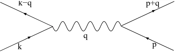
by this veretex to the S matrix elements in the subspace of electron states. This is shown in Fig. 1. It describes the exchange of a transverse photon between two transverse electron currents mediated by the transverse photon propagator given in the 4-dimensional Fourier spaceω, ~qby
1
q2−ω2/c2−ı0(δµ,ν−
qµqν
q2 ); (µ, ν= 1,2,3)
and the vertices contain momentum factors corresponding to the the currents (see Ref. [4] )
After neglecting the term −ω2/c2 in the denominator (i.e. ignoring retardation) one eliminates
cor-rections of higher order as 1/c2 and the photon propagator looks as 1
q2(δµ,ν−
qµqν
q2 ); (µ, ν= 1,2,3) .
Since no pole survived, the −ı0 term could have been also ignored and 4qπ2 is just the Fourier transform
of the Coulomb potential.
k
p
q
p+q
k−q
Figure 1: The basic electron current-electron current (transverse photon exchange) graph in QED.
Then one may convince oneself that these graphs coincide with the basic vertexes of the S matrix of an 1/c2 purely electron Hamiltonian containing besides the kinetic energy and the Coulomb interactions
the interaction term
−1 2 Z
d~x Z
d ~x0N h
~i⊥(~x)~i⊥(~x0)i
c2|~x−~x0| . (41) This term has an appealing form analogous to the charge density-charge density Coulomb interaction. It is the microscopical expression of the important Biot-Savart law of interaction between currents in finite macroscopic samples, where light propagation effects may be ignored.
In order to keep gauge invariance with respect to an external field Aext~ one has to use again the minimal recipe and this requires also its introduction not only in the kinetic energy term, but also in the current-current interaction.
This transverse current-current interaction Eq. 41 was first derived in Ref.[4] both within this QED frame, as well as within Landau’s construction based on the classical theory of point-like charges in the Coulomb gauge.
8
Conclusions.
Acknowledgement.
The first author has to express his gratitude to Peter Kopietz for bringing his attention to Ref. [5] and useful discussions on this subject.
References
[1] C.G. Darwin, Phil. Mag. ser. 6.36, 537 (1920)
[2] L.D. Landau and E. M. Lifshitz, The Classical Theory of Fields. Pergamon Press, 1971
[3] D. N. Zubarev, Nonequilibrium Statistical Thermodynamics, Consultants Bureau, 1974 (russian edition in 1971)
[4] L.A. B´anyai, arXiv:1905.02390v5 (2019)
[5] T. Holstein, R.E. Norton and P. Pincus, Phys. Rev.B 2649 (1973)
[6] Ladislaus Alexander B´anyai, A Compendium of solid-state theory, (Springer International (2018)
[7] P. A. M. Dirac, Can. J. Math.2,147 (1950)