ABSTRACT
KALLITSIS, MICHAEL G. Optimal Resource Allocation for Next Generation Network Services. (Under the direction of Michael Devetsikiotis.)
Advances in various networking and computing technologies that allow high bandwidth, low latency connections have made transport services offered by telecommunication service providers to become a commodity. In order to gain a competitive advantage, service providers seek to enable value-added, next generation network services layered on top of the commodity transport service. At the same time, businesses across industries realize the need to be flexible and adapt to change so as to succeed in today’s information-driven economy. A robust, efficient, scalable, and dynamic communication and integration infrastructure is necessary to support this trend.
Next generation network services include services that are offered via the emerging service oriented network architectures, such as e-banking and e-commerce transactions, security ser-vices and communication serser-vices with users’ presence and location information. In addition, the evolution of the “Web 3.0” paradigm provides services like online social networks, virtual collaborative environments and cloud computing services. Moreover, services like voice over IP, video on demand, online gaming and high speed Internet services are brought through triple and quadruple play architectures. Those services have diverse quality-of-service requirements and are constantly evolving in size while being geographically distributed across the world. Hence, network and system designers encounter the challenge of allocating the scarce and lim-ited network and computing resources in an efficient and fair manner.
c
Optimal Resource Allocation for Next Generation Network Services
by
Michael G. Kallitsis
A dissertation submitted to the Graduate Faculty of North Carolina State University
in partial fulfillment of the requirements for the Degree of
Doctor of Philosophy
Computer Engineering
Raleigh, North Carolina 2010
APPROVED BY:
Do Young Eun Ioannis Viniotis
William Stewart George Michailidis
University of Michigan, Ann-Arbor
DEDICATION
StougoneÈmou,Gi°rgo kaiPand°ra,kaisthn adelfmouGalteia.
BIOGRAPHY
The author was born in the island of Cyprus, on July of the year one thousand nine hundred and eighty.
He graduated from the Gymnasium of Pallouriotissa and he was a recipient of student ex-cellence awards during his whole studies. His inclination to mathematics and other physical sciences, along with the strong support from his family, motivated Michael to apply for un-dergraduate studies to the prestigious and highly competitive National Technical University of Athens (Metsovio) in Greece.
He was accepted and proceeded towards this new step of his life after serving the obligatory military service for his country. After five wonderful, exciting and, also, on some occasions, difficult years in Athens (Michael’s father, George, left this world during Michael’s third year of studies), he obtained his Undergraduate Diploma (five-year degree) from the School of Electrical and Computer Engineering majoring in Communications, Networks and Computer Systems, ranked in the top 3% of his class.
The new challenge was a graduate degree in the field of communication networks. Michael decided to apply in several universities across the United States of America. It was a destination that the author was not even imagining a couple of years earlier. God, luck or destiny (you name it), guided Michael to apply to North Carolina State University. He was contacted by Professor Michael Devetsikiotis to join his research group, namely the Network Performance Research Group. Michael accepted the offer and flew to Raleigh, North Carolina for his new endeavors on the summer of the year two thousand and five.
ACKNOWLEDGEMENTS
This dissertation could not have been completed without the help and guidance of my thesis advisors, Professor Michael Devetsikiotis and Professor George Michailidis. The chemistry of our cooperation has been proven to be very successful and they helped me complete my work without having to worry about stressful deadlines very often. In addition, the financial aid I was provided during my whole stay at NCSU, has been a major relief and motivation for completing my degree. Special thanks go to the other members of my PhD committee, Professor Do Young Eun, Professor Ioannis Viniotis and Professor William Stewart for their valuable comments and feedback for my dissertation. I should not forget to mention Professor Harry Perros for his kind assistance in queueing theory concepts as well as in other personal matters while I was pursuing my degree. Moreover, special acknowledgments should be sent to Professor Mitzi Montoya for our cooperation in the social aspects of virtual collaborative environments.
Regarding people outside the world of NCSU, I would like to express my sincere appreciation to Dr. Robert Callaway, a friend and colleague, for all the valuable discussions we had and the help he provided in almost every step of my doctorate. I wish to express my gratitude to Dr. Adolfo Rodriguez and Dr. Robert Frazier for their help and support during my internship experience at IBM and Ericsson, respectively. Their guidance and the responsibilities I was assigned during my internships helped me to acquire valuable tools for my academic research. I would also like to acknowledge Professor Stilian Stoev, University of Michigan, for his help regarding network traffic estimators in Matlab. Moreover, I should not forget to mention my appreciation to ”Korgialenion Athlon” Foundation for the scholarship I have been awarded.
TABLE OF CONTENTS
List of Tables . . . vii
List of Figures . . . .viii
Chapter 1 Introduction . . . 1
1.1 Motivation . . . 2
1.1.1 Service Oriented Networks . . . 2
1.1.2 The Web 3.0 paradigm . . . 3
1.1.3 Triple Play Services . . . 5
1.2 Contributions . . . 5
Chapter 2 Centralized Optimization in Service Oriented Networks . . . 8
2.1 Related Work . . . 10
2.2 Modeling Framework . . . 11
2.3 Pricing Model and Problem Formulation . . . 12
2.3.1 Non-linear optimization model with pricing differentiation . . . 13
2.3.2 Convex optimization . . . 16
2.4 Online Traffic Measurement and Traffic Monitoring . . . 19
2.5 Performance Evaluation . . . 21
2.5.1 Sensitivity to Model Parameters . . . 22
2.5.2 Assessing the dynamic behavior of MBORA . . . 26
2.5.3 Evaluation of traffic monitoring and estimation . . . 28
2.5.4 Evaluation with real traffic data (Abilene traces) . . . 32
2.6 Conclusion . . . 35
Chapter 3 Distributed Algorithms for Optimization in Service Oriented Net-works . . . 37
3.1 A Framework for Delay Sensitive SON . . . 39
3.1.1 Formulation of Optimization Problem . . . 40
3.1.2 Online Traffic Monitoring . . . 43
3.2 Distributed Optimization Algorithms . . . 43
3.2.1 Distributed Algorithm based on Dual Decomposition . . . 43
3.2.2 Distributed Algorithm based on Gauss-Seidel iterations . . . 46
3.3 Performance Evaluation . . . 48
3.3.1 Evaluation of Algorithm I - dual decomposition based algorithm . . . 49
3.3.2 Evaluation of Algorithm II - Gauss-Seidel based algorithm . . . 50
3.3.3 Dual Decomposition Vs. Gauss-Seidel . . . 51
Chapter 4 Optimization using Bounds from Network Decomposition . . . 59
4.1 Introduction . . . 59
4.2 Network Decomposition . . . 61
4.2.1 Background Theory . . . 61
4.2.2 Recursive Formulas - An Introduction . . . 64
4.2.3 Recursive Formulas for general network topologies . . . 65
4.2.4 Discussion on algorithm’s complexity . . . 69
4.3 Optimal Resource Allocation . . . 71
4.3.1 Heuristic for feasible θ’s . . . 72
4.4 Performance Evaluation . . . 72
4.4.1 Sensitivity analysis on a two-node tandem network . . . 73
4.4.2 Network Decomposition Vs. Network Calculus . . . 74
4.4.3 Topologies with fork/join operations . . . 78
4.5 Conclusion . . . 82
Chapter 5 Multiple Resource Allocation in Social Networks . . . 83
5.1 Related Work . . . 85
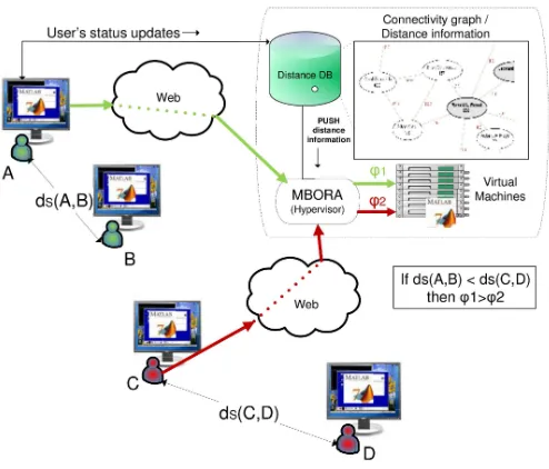
5.2 Connectivity graph and social distance . . . 86
5.3 Optimum Allocation of Multiple Resources . . . 89
5.4 Performance Evaluation . . . 90
5.5 Discussion: techno-social interaction . . . 93
5.5.1 Techno-Social Interaction Measures . . . 94
5.5.2 Incorporating Techno-Social Interactions in Resource Allocation Problems 95 5.5.3 An Integrated Formulation of Techno-social Optimization Problems . . . 99
5.6 Conclusion . . . 101
Chapter 6 Conclusions . . . .102
Bibliography . . . .104
Appendices . . . .113
Appendix A Wavelets . . . 114
Appendix B Network Calculus . . . 116
B.1 The Basics . . . 116
B.2 Service Curves . . . 117
Appendix C Incorporating CPU processing delay of SON appliances . . . 119
LIST OF TABLES
Table 2.1 Parameters of each service classi(i= 1,2) . . . 23
Table 2.2 Changing the pricing factorpi. . . 24
Table 2.3 Sensitivity to Hurst parameter Hi. . . 24
Table 2.4 Sensitivity to mean arrival rate ¯αi. . . 26
Table 2.5 Sensitivity to pricing parameterpi. . . 26
Table 2.6 Responsiveness to traffic changes. Evaluating the dynamic behavior of MBORA. . . 27
Table 2.7 Traffic estimation, allocation and utility for the Abilene traces case study. 35 Table 2.8 Traffic estimation, allocation and utility for the FGN traces case study. . . 35
Table 3.1 Parameters of each service classi(i= 1,2, . . . ,5) . . . 51
Table 3.2 Comparison of GS and Dual using real life IM data. . . 57
Table 4.1 Comparing network calculus and network decomposition. . . 75
Table 4.2 Optimal resource allocation (whenσ = 100Kb). Note that violation prob-ability increases (i.e., exponent decreases) as cross traffic rate increases. Note, also, that our heuristic yields a close to optimal solution. . . 81
Table 5.1 Connectivity graph parameters for application-k,k∈ {α, β, γ} . . . 91
Table 5.2 Sensitivity on resource demand (ωi0, ψ0i) . . . 92
LIST OF FIGURES
Figure 1.1 Content-based routing . . . 4
Figure 1.2 Allocation of resources in a virtual collaboration environment. . . 5
Figure 1.3 Network Transformation: increased bandwidth requirements (from [2]) . . 6
Figure 2.1 Depiction of the proposed framework: traffic is divided into two cate-gories; deterministic constraint and elastic constraint services. The sys-tem allocates the excess resources to the latter set. . . 12
Figure 2.2 The MBORA system: the optimization module receives as input the traf-fic measurements made by the measurement module. It calculates the optimal resource allocation when an out-of-control signal is triggered. The solution is then passed to the resource orchestrator (scheduler). . . . 13
Figure 2.3 Our cost function. Notice that even a small increase of 2.5% above the delay threshold yields an increase above 100% in the cost function. In this case, βi= 10. . . 14
Figure 2.4 Graphical interpretation of the probabilistic queue bound qmax . . . 17
Figure 2.5 The Exponentially Weighted Moving Average Chart. . . 21
Figure 2.6 Concavity of our utility function . . . 23
Figure 2.7 Sensitivities to mean arrival rates ai and delay thresholddi . . . 23
Figure 2.8 Allocation using an average delay metric versus the allocation using our stochastic delay metric. . . 25
Figure 2.9 MBORA vs. Oracle-I: evaluation of EWMA’s sensitivity to traffic shifts (see discussion in subsection 2.5.3) . . . 28
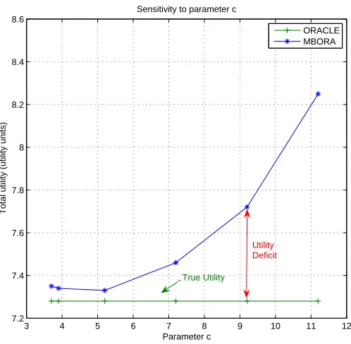
Figure 2.10 Sensitivity of EWMA to parameter c. The Oracle-I system yields a precise total utility whereas MBORA has a utility deficit according to the value of c. . . 29
Figure 2.11 A simple scenario of traffic changes: traffic of service class 1 is not changed whereas changes of service class 2 are captured by the MBORA system. . 31
Figure 2.12 MBORA vs. Oracle-II: evaluation of our traffic estimator (see discussion in subsection 2.5.3) . . . 33
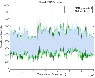
Figure 2.13 EWMA control on the Abilene and the FGN traces. Note that the major traffic changes are captured. . . 34
Figure 2.14 Comparison of Abilene Vs. FGN generated traces for service class 1. . . . 34
Figure 3.1 High level architecture of the proposed system. . . 40
Figure 3.2 Simple topology. The two nodes exchange their local solutions until our convergence criteria are met. . . 48
Figure 3.3 The network topology used in our scenarios with IM data. Class-itravels from Si to Di. . . 49
Figure 3.4 Sensitivity to pricing parameter p1 and delay thresholdd1. . . 50
Figure 3.6 Sensitivity to pricing parameter p1. . . 52
Figure 3.7 Sensitivity to delay threshold d1. . . 52
Figure 3.8 Optional caption for list of figures . . . 53
Figure 3.9 Asynchronous convergence of Gauss-Seidel algorithms. . . 54
Figure 3.10 Structured topologies for signalling comparison (section 3.3.3). . . 56
Figure 3.11 Message exchanges between nodes in the Dual algorithm. . . 57
Figure 4.1 Network elements in tandem with capacityN ceach traversed bynthrough flows and N−ncross flows. . . 63
Figure 4.2 The join, fork and tandem operators. In join, flows from different paths meet. In fork, flows coming from the same path split. Tandem is a subcase of the join operation. . . 66
Figure 4.3 An example network topology. Here, ∆1 = {γn11,γn¯ 11, n12}, ∆2 = {n21, n22}, ∆3 ={Γ3,∆2}={γn11,¯γn11,∆2} and ∆4={n41, γn11}. . . . 67
Figure 4.4 The fork operator is a subcase of the join operator. . . 68
Figure 4.5 A full binary tree topology with join operators. . . 70
Figure 4.6 Visual illustration of our heuristic for finding the feasible θ’s. . . 73
Figure 4.7 Sensitivity to peak rate. . . 75
Figure 4.8 Sensitivity to backlog. . . 76
Figure 4.9 Concatenation of service curves in network calculus. . . 76
Figure 4.10 Advantages of network decomposition over network calculus. . . 77
Figure 4.11 Sensitivity to peak rate P (σ = 100K, µ1 = 1ms, 1λ = 9ms.) . . . 78
Figure 4.12 Sensitivity to routing ratio γ. . . 79
Figure 4.13 Sensitivity to incoming flows n1. Loose bounds can sometimes appear. . . 80
Figure 4.14 Sprint over-provisioning allocation scheme. . . 80
Figure 5.1 Allocation of resources in a virtual collaboration environment. . . 84
Figure 5.2 The connectivity graph used to represent each virtual world. Note that the graph should a complete one; for visual brevity, here it is not. . . 87
Figure 5.3 Differentiating the connectivity graph using the average sum of edge weights. 88 Figure 5.4 Obtaining presence information from the connectivity graph. . . 89
Figure 5.5 Sensitivity on the physical distance. . . 92
Figure 5.6 Sensitivity to pricing parameter χk of application-α. . . 93
Figure 5.7 An example of users collaborating in a corporate network. . . 97
Figure B.1 Bounds on backlog and delay. . . 118
Figure C.1 CPU and network queues of two SON nodes in tandem. . . 120
Chapter 1
Introduction
Advances in various networking and computing technologies that allow high bandwidth, low latency connections have made transport services offered by telecommunication service providers to become a commodity. In order to gain a competitive advantage, service providers seek to enable value-added, next generation network services layered on top of the commodity transport service. At the same time, businesses across industries realize the need to be flexible and adapt to change so as to succeed in today’s information-driven economy. A robust, efficient, scalable, and dynamic communication and integration infrastructure is necessary to support this trend. Next generation network services include services that are offered via the emerging service oriented network architectures, such as e-banking and e-commerce transactions, security ser-vices and communication serser-vices with users’ presence and location information. In addition, the evolution of the “Web 3.0” paradigm provides services like online social networks, virtual collaborative environments and cloud computing services. Moreover, services like voice over IP, video on demand, online gaming and high speed Internet services are brought through triple and quadruple play architectures.
chapters that follow.
1.1
Motivation
We provide some insights about the motivation of our work. We begin by describing service oriented network services and then we proceed to services belonging to the Web 3.0 kingdom, such as cloud computing services, social networking and virtual collaboration. We conclude with triple play services.
1.1.1 Service Oriented Networks
Service Oriented Networking (SON) is a blooming architecture that provides intelligent
func-tionality in the network [1]. This kind of networks belong to the category of application-aware networks; i.e., an emerging technology where traffic is treated based on the application data. This technology seeks to increase the end-to-end performance of next generation network ser-vices. It is accomplished by allowing routers and other network appliances to inspect the appli-cation data contained in packets. The Extensible Markup Language (XML) [2] has nowadays become the proper standard to ease the implementation of that networks [3].
The need for a SON arose due to the tremendous spreading of the Service Oriented Architec-ture (SOA) in corporations. The SOA ”affords new levels of agility and flexibility over legacy architectures by resolving the complexity and inflexibility of traditional middleware through open standards and a more loosely coupled approach to designing, developing, and deploying applications” [3]. That is, the SOA allows different systems to interact with each other without caring about the underlying architecture/protocol details of their communicating partner; the interaction is made using a loosely coupled, message-based communication model.
The key ingredient is a network device that is highly ”smart”, able to understand what kind of services flow through itself. Understanding the traffic and acting accordingly to in-coming requests and responses is critical to successful SOA deployment. This can be achieved via intelligent network devices, called Network Service Intermediaries (NSI) (also named ”mid-dleboxes” and ”proxies”), which can prioritize requests based on rules and logic, removing the burden from the application servers that support the requests. Examples of NSIs include IBM’s DataPower Service Oriented appliances [4] and CISCO’s Application Oriented Network (AON) message routing systems [5].
policies that respect application-specific goals. For example, messages of a certain type may be routed or transformed in a certain way. CBR (also called intelligent routing) is a functionality that can be exploited for pricing and optimizing networks. Figure 1.1 illustrates an example where we have a differentiation of service requests. In that example, we have a total of three service classes having different priorities.
Before getting into the actual details of our example let us first introduce an interesting result from the academic literature. In [6] the authors claim that e-commerce HTTP sessions that have existed for more than 60 seconds generally belong to customers who are willing to make a purchase through the web site. Thus, in our example, we partition e-commerce service requests into two categories: (a) e-commerce sessions that have lived for more than 60 seconds and (b) ”younger” e-commerce sessions.
We have the following case study: suppose that e-commerce providers (e.g., Amazon, eBay) sell their product to the daily growing population of e-shoppers. Assume that the incoming requests are processed through the SON appliance shown in Figure 1.1. The serving node accepts three kind of requests: the two classes of e-commerce sessions that we mentioned above and a management session. These services with different priorities and thus different QoS requirements (e.g., delay requirements). Thus, our content-aware device should allocate the resources accordingly: the more important e-commerce sessions will be given more network resources to satisfy their strict QoS requirements (e.g., these requests can be routed to servers hosting the service that are optimized for high demand scenarios). The other services will be directed to separate servers and will be given less resources. This class differentiation can be accomplished using XPath routing. With XPath routing we can look inside the application layer XML data, search for the information of interest (e.g., the age of the e-commerce session) and route accordingly the messages to the appropriate destination.
1.1.2 The Web 3.0 paradigm
The Web 3.0 is a term implying the future use of the World Wide Web (WWW) by software
developers and end-users. It follows the introduction of the phrase ”Web 2.0” that describes the trend of a more interactive Internet with content-rich web portals, wikis, blogs, social-networking sites, instant messaging and communication among users and various collaborative tools. Characteristic applications that belong to the Web 3.0 paradigm include online social networks (e.g., Facebook [7], Twitter [8], MySpace [9], Flickr [10]), collaborative 3D environ-ments via online virtual worlds (e.g., Second Life [11], Qwaq [12], Wonderland [13]) and cloud
computingapplications such as the Virtual Computing Lab (VCL) initiative, Google documents
and the Amazon EC2 cloud.
Figure 1.1: Content-based routing
an example of an optimal resource allocation framework for such applications. A virtual world is a simulated environment in which multiple users inhabit and interact via human-like forms, called avatars. The user remotely accesses a computer-simulated world and allows people to manipulate elements of the modeled world. The modeled worlds may appear similar to the real world or instead represent imaginary worlds. Communication between users may vary from text to gestures or sound and video. The virtual world paradigm can be applied in team work (i.e., virtual collaboration and meetings), education, gaming, social networking, training employees as well as for commercial purposes.
Figure 1.2: Allocation of resources in a virtual collaboration environment.
1.1.3 Triple Play Services
The Triple Play is a marketing term for the provisioning of three services; high speed
Inter-net, television (Video on Demand or regular broadcasts) and telephone service over a single broadband connection. It is obvious that a network transformation is required for triple play services. The solution for voice is trivial; since voice has small bandwidth requirements we can alleviate all the problems by just reserving some network capacity for it. However, with the video service - which includes IPTV, Video on Demand and high definition TV - things are not so apparent. Users may now need up to 20Mbps to satisfy their needs. A study from Alcatel (see Figure 1.3 - reprinted from [14]) has indicated a huge bandwidth increase in different por-tions of the network compared to today’s requirements. Ideas like multicasting the video with a protocol called IGMP (Internet Group Management Protocol) have emerged but may not be sufficient. As a result, we realize that triple play postulates the need for efficient resource allocation schemes that can take into account the price of each service, its quality-of-service requirements and the available scarce resources across all network elements. Traffic could be categorized using deep-packet inspection techniques.
1.2
Contributions
Figure 1.3: Network Transformation: increased bandwidth requirements (from [2])
spending our time on various optimization methods, queueing theory and other performance analysis tools, traffic monitoring and characterization as well as simulation efforts by articulating the problem that this dissertation tries to address.
Problem Definition. We are given a finite amount of resources along with some constraints that could be either technical constraints (e.g., delay requirements or other quality-of-service metrics) or non-technical (e.g., social constraints). We are responsible for allocating those resources to network services or other types of computing applications. How can we optimally allocate those resources to the interested services so as to meet the performance requirements and the constraints at the best possible degree?
We address instances of the above problem from different angles as follows:
• Chapter 2 introduces our Measurement-based Optimal Resource Allocation (MBORA) framework that is responsible for dynamic and optimal resource allocation in a centralized manner at a single network element in service oriented networks. We employ probabilistic delay bounds to assess the performance of each service class. Traffic is characterized using the fractional Brownian motion model. The model is evaluated using real life network traces taken from the Abilene network. Our scientific publications on the subject are [15, 16, 17].
that incorporates a cost component based on a network calculus metric, which to the best of our knowledge, is the first attempt to integrate such a metric into a network utility maximization formulation. In addition, we present two distributed optimization algorithms and scrutinized comparisons of them, including evaluation with real world instant messaging traffic data. Relevant publications include [18, 19, 20].
• In Chapter 4, we utilize network decomposition tools and construct recursive relations that ease the derivation of input and output traffic envelopes at every node. Based on those, the backlog bound metric for the flows can be acquired and an explicit algorithm is provided to achieve that. This bound is then integrated into a resource allocation optimization problem. Experimental juxtapositions against a) network calculus and b) static over-provisioning schemes reveal the advantages of the proposed scheme. This work is also presented in [21].
• Chapter 5 deals with optimization in social networks and, in particular, virtual collab-orative environments. We introduce the metric of social distance that incorporates the social and technical interactions between the participants of a virtual environment that utilize a particular application. We build a utility-based framework that considers the social distance and optimally allocates the available computing resources. Our formula-tion includes multiple resources and, hence, we consider multidimensional Knapsack-type placement problems. This study is also discussed in [22].
Chapter 2
Centralized Optimization in Service
Oriented Networks
In this chapter, we introduce a model that ensures efficient resource allocation, while maximizing the provider’s utility in service-oriented networks. Our model considers a pricing scheme for the offered services and the quality of service (QoS) requirements of each service class, which operates under a probabilistic delay bound constraint.
Our work is motivated by the immense advances in the information technology sector which have led telecommunication providers to enrich their service portfolio with value-added services so as to drive the success of their businesses. Plain transport services are not profitable and, hence, services such as triple/quadruple play, multimedia messaging and presence are emerg-ing via the service-oriented architecture paradigm, which is the foundation for next-generation telecommunication networks. Furthermore, services offered through virtual environments con-stitute another trend; specifically, people get the opportunity to utilize applications that de-mand significant computing resources and expensive licensing using remote high performance servers [23] or even attend lectures and presentations being offered via virtual worlds [12].
The above services require careful management of the available network (e.g., bandwidth, network storage) and computing resources (e.g., memory, CPU capacity). Allocation of re-sources should be done optimally and dynamically, since static sharing can lead to under-utilization of the network infrastructure. In this chapter, we concentrate on the optimal allo-cation of a single network resource.
will need hardware-accelerated, content-aware tools to process the contents of application mes-sage payloads and take various policy-driven actions in response to what they find. The idea of computations on messages passing through network elements was first introduced in active
networks and a survey can be found in [26]. Application-level awareness is also discussed in [27]
and is considered to be of key importance in future Internet design. Such awareness can be employed on web services like e-commerce, web auctions, stock quotes and banking transac-tions that exhibit delay sensitive characteristics. The delay sensitive nature of such services may play a critical role on whether the transaction will be eventually completed or not; users experiencing long delays are eager to postpone or even desist the procedure. Therefore, it is in the provider’s best interest to enhance the quality of experience of such activities.
The aforementioned service quality improvement can be achieved by adopting an optimal resource allocation scheme like the one proposed next. In our scheme, pricing is used to attain service differentiation based on the priority and the value of each service. We also employ online feedback control that evaluates the performance of each service class based on the current traffic characteristics and the desired QoS specifications and reacts accordingly. Moreover, we leverage an exponentially-weighted moving average (EWMA) control scheme to predict imminent arrivals and capture significant traffic changes. We assume a fractional Brownian motion (fBm) traffic model because of its ability to adequately capture characteristics of Web traffic, such as self-similarity and the presence of heavy tailed marginal distributions. (See Crovella et al. [28] for the ubiquitous presence of self-similarity in Web traffic and [29] for self-similarity of Ethernet traffic.) Further, evidence of self-similar phenomena in e-commerce HTTP traffic is established in [30].
2.1
Related Work
Our flow control methodology follows along the lines of the seminal papers by Kellyet al.[31, 32] in which the network utility maximization (NUM) problem is analyzed. Their major contri-bution is the proposal of a distributed algorithm, that yields a fair allocation of the network resources. In addition, the algorithm is stable in the sense that it will always converge to a solution despite any possible perturbations on the information that the algorithm collects from the network. The model presented in this chapter differs from Kelly’s work; we study a single network resource and the optimization is solved in a centralized fashion. A distributed allocation of multiple network resources is part of ongoing work.
Flow control has been studied extensively in the context of wired networks [33, 34, 35, 36, 37, 38, 39, 40]. In [33], an optimization approach to flow control is presented, where the goal is to maximize the total utility of all sources over their transmission rates. The basic algorithm solves the dual problem and involves links calculating bandwidth prices and sources selecting rates based on current link prices. In [34], the authors investigate the problem of allocating transmission data rates to users in the Internet in a distributed fashion. In addition to the customary concave utility functions, they propose the use of sigmoidal (non-concave) ones as appropriate for capturing the elasticity of delay sensitive services, like video and audio. Therefore, a non-convex optimization problem needs to be addressed. In [35], the authors study the utility maximization problem in networks where flows arrive and depart dynamically (as opposed to Kelly’s work where flows appear to have infinite backlog to transfer). Their objective is to maximize the long-term expected system utility, under the link capacity constraints. In [36], a game-theoretic framework for bandwidth allocation for elastic services (an elastic service is defined as a service that can modify its data rate according to the available bandwidth within the network) is proposed and a distributed algorithm that yields the optimal and fair allocation is provided. In [37], the authors propose to maximize a utility function specified by the network subscribers and resources are shared based on the solution of that optimization problem. The above papers are mostly concerned about congestion control on the Internet (e.g., a typical application of rate control appears in the TCP traffic context). Nevertheless, studies based on the NUM framework have emerged for power control and rate adaptation in wireless networks [41, 42], MAC protocol [43], etc. A nice tutorial on cross-layer optimization can be found in [44].
compared to the one obtained through stochastic delays. In [39], network utility maximization is achieved through utility functions that incorporate the delay requirements of incoming traffic classes and distributed algorithms are proposed for the solution of the optimization problem. However, the work does not address the frequency and the conditions for solving the resulting optimization problem. In addition, they rely on the not-so-reliable average delay metric. Con-gestion management in a network where users have different delay requirements is also studied in [40].
The online traffic control part of this work utilizes the EWMA control scheme [45]. EWMA has been considered in [46] where the authors monitor traffic intensities so as to optimally allocate the resources of a Switched Processing System (SPS - a SPS represents a canonical model of systems characterized by the flexible service requirements of incoming traffic flows). Traffic measurements play also a key-role in [47] for setting the optimal pricing scheme that maximizes social welfare using traffic monitoring. Similarly, an optimal measurement-based pricing scheme for M/M/1 queues, where the total charge depends on both the mean delay at the queue and arrival rate of each customer is presented in [48].
2.2
Modeling Framework
The employed modeling framework was introduced in [38] and is depicted in Figure 2.1. In its present form it represents a single network element, which may correspond to either a traditional network component, such as a switch or a router, or a modern network “service center”, like IBM’s Datapower service-oriented network appliances [24] or Cisco’s application-oriented network message routing systems [5].
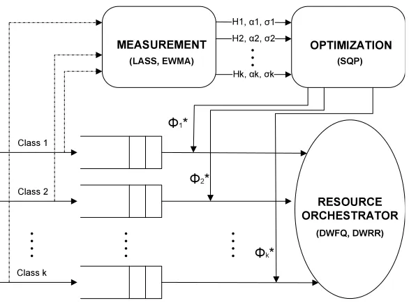
It is assumed that the network element serves two categories of traffic classes; deterministic bound classes and flexible bound ones. Due to the fact that deterministic delay-bound classes have strict requirements, their service level agreement (SLA) can be satisfied only by traffic shaping and admission control schemes; the interested reader can refer to [49, 50, 51, 52] and the references therein for a discussion on QoS and admission control. Thus, a certain amount of resources is dedicated to them and these classes are excluded from subsequent analysis. Examples of such inelastic classes of service include teleconferencing, remote seminars, real-time distributed computation/simulation and high-precision medical imaging.
Hence, the proposed system is responsible for optimally allocating the excess resources to the remaining flexible delay-bound classes (e.g., web services). These classes enter the measurement-based optimal resource allocation (MBORA) system which is illustrated in Figure 2.2. The MBORA system consists of a measurement module, an optimization module and a resource
orchestrator module. The statistics of the arrival traffic are measured by the measurement
Figure 2.1: Depiction of the proposed framework: traffic is divided into two categories; deter-ministic constraint and elastic constraint services. The system allocates the excess resources to the latter set.
which can account for the burstiness and long-range dependence (LRD) observed in real network traffic traces. Such a model can be fully described by the following parameters: the Hurst
parameterHthat captures the dependence structure, the mean arrival rate ¯α and thevariance
σ of the marginal distribution.
The optimization module receives the traffic characteristics of each class and calculates the optimal allocation of resources by solving the optimization problem discussed in Section 2.3. In order to avoid excessive computations, the optimization problem is solved only when significant changes in the traffic characteristics are detected. The latter is accomplished by employing an exponentially weighted moving average (EWMA) control chart, which signals when the estimated traffic intensity ¯α goes out-of-control by exceeding some pre-specified bounds. The calculated optimal solution is subsequently fed to the resource orchestrator which dynamically updates the allocation of resources for each traffic class and forwards the packets (or, more generally, the messages, for example XML) towards their destination.
2.3
Pricing Model and Problem Formulation
MEASUREMENT OPTIMIZATION
RESOURCE ORCHESTRATOR
Class 1
Class 2
Class k
H 1, α1, σ 1
Η2, α2, σ2
Ηk, αk, σk
Φ1*
Φ2*
Φk*
(LASS, EWMA) (SQP)
(DWFQ, DWRR)
Figure 2.2: The MBORA system: the optimization module receives as input the traffic measure-ments made by the measurement module. It calculates the optimal resource allocation when an out-of-control signal is triggered. The solution is then passed to the resource orchestrator (scheduler).
2.3.1 Non-linear optimization model with pricing differentiation
Suppose that the node can accommodate K different types of services. The proportions of resources to be allocated to the K types are denoted by φ= (φ1,· · ·, φK). According to [53],
the profit of a provider is the difference between the revenuer(φ) obtained from providing the services (i.e., usage-based pricing), and the cost c(φ) that incurs from producing them. The aim of the provider is to maximize the profit function π:
π =max
φ {r(φ)−c(φ)}=maxφ K
X
i=1
(ri(φi)−ci(φi)), (2.1)
subject to the feasibility constraints: φk≥0, i= 1,· · · , K, Piφi≤1.
Specifically, ri(φi) = pi·φi, while the cost function takes the form ci(φi) = bi ·Di(φi)· exp[βi(Di(φi)−di)]. The coefficient pi corresponds to the price charged by the provider for the ith service, whilebi is the amount the provider has to reimburse the users whenever their SLAs
are not satisfied. A higher priority class u requires better service than a lower one v and thus it is charged accordingly (i.e., pu > pv and bu > bv). The parameter βi controls the steepness
of the cost function, whileDi(φi) denotes the value of the performance metric experienced by
3.7 3.8 3.9 4 4.1 4.2 4.3 4.4 0
10 20 30 40 50 60 70 80 90
Delay Di(φi)
Cost Funtion c
i
(
φ i
)
Cost Function, delay threshold d
i=4
← threshold
Figure 2.3: Our cost function. Notice that even a small increase of 2.5% above the delay threshold yields an increase above 100% in the cost function. In this case, βi = 10.
We adopted a linear form for the revenue function so as to represent the bandwidth profit
(i.e., product of price times bandwidth allocated) that a provider would receive. In addition, linearity offers concavity and simplicity which are required characteristics for our optimization problem formulation. On the other hand, our cost function has a nonlinear form (Figure 2.3). The exponential shape allows a more severe penalization (i.e., a cost penalty) of the provider, when services experience larger queue delays than those agreed under the SLA. For example, if
Di(φi)> dithe users are not receiving adequate resources from the provider, which would incur
a cost, until the situation is rectified. Figure 2.3 shows a steep increase in the cost function when the delay exceeds the desired threshold di. This would force the provider to adjust the
allocation of resources, if possible, in order to satisfy the requirements and maximize profit. If the system is already highly utilized and the re-allocation of resources cannot alleviate the incurred cost, the provider should consider acquiring more resources.
It should be noted that prices cannot buy a specific QoS performance. Prices are used as a priority parameter for each service-iand the intuition is that the service that pays more will get more bandwidth (allocation also depends on the QoS ǫi and the delay threshold di). In
The Probabilistic Queue Bound
We employ stochastic delay bounds as our QoS metric. Specifically, we adopt the approach used in [54, 55], where traffic is treated as LRD and is characterized by the Hurst parameterH, the mean ¯α and the variance σ. It is shown that the queue length Qi(t;φi) at any given time t
is bounded by a valueqi,max with probability ǫi >0 related to the desired QoS. In particular,
for a specific class-ithe following holds:
P r{Qi(t;φi)> qi,max(φi)} ≈ǫi (2.2)
and
qi,max(φi) = (φiC−α¯)
Hi Hi−1(k
iσi) 1 1−HiH
Hi
1−Hi
i (1−Hi), (2.3)
where φiC can be interpreted as the resources (e.g., bandwidth, CPU, etc.) dedicated to this
particular class,ǫi the required QoS andki=√−2lnǫi.
Thus, since the queue length and expected delay are related using the generalized Little’s law, we have the following probabilistic delay bound for a FIFO queue:
P r{Di(t;φi)> Di,max(φi)} ≈ǫi, (2.4)
where Di,max(φi) =qi,max(φi)/φiC. For simplicity, in our cost function we refer toDi,max(φi)
asDi(φi). We have a SLA violation if at given traffic conditions ¯αi,σi and Hi, the stochastic
delay bound, Di(φi), for the agreed QoS, ǫi, is greater than the desired delay bound di. A
stricter QoS implies a smaller value of ǫi that generates a larger Di(φi). Hence, the SLA is
more likely to be violated for a given delay thresholddiand, therefore, the provider is motivated
to allocate more resources to that service class.
We give a sketch of the proof for the probabilistic queue bound shown in equation 2.3 and offer some insights about its use. For a rigorous mathematical proof the reader should refer to [54, 55]. First, we need to defineQ(t) as the queue length at timetand AH(t) as the arrival
process at the queue of interest. We consider that the queue length at time, Q(t), exceeds the maximum queue length, qmax, with probability ǫ. This probability is equivalent to the
probability with which the arrival process, AH(t), exceeds the envelope arrival process, ˆAH(t).
In other words:
P r{Q(t)> qmax}=P r{AH(t)>AˆH(t)} ≈ǫ
In our model, the envelope process is defined as ˆAH(t) = ¯αt+kσtH and represents a
Parameter kdetermines the probability that AH(t) will exceed ¯AH(t) at timet. We have
P r{AH(t)>AˆH(t)}=P r{
AH(t)−αt¯
σtH > k}= Φ(k)
where Φ(x) is the residual Gaussian distribution function. Using the approximation Φ(x) ≈
exp(−x2/2) we find thatk=p−2ln(ǫ) such that Φ(k) =ǫ.
By defining ˆQ(t) as ˆQ(t) = ˆAH(t)−Ct≥ 0, we can compute qmax by finding the time t∗
that maximizes ˆQ(t). Thus, we need to solve dQˆdt(t∗) = 0 which yields:
t∗ = [ kσH
(C−α¯)]
1/(1−H) (2.5)
Substitutingt∗ intoq
max= ˆAH(t∗)−Ct∗ yields:
qmax = (C−α¯)H/(H−1)(kσ)1/(1−H)HH/(1−H)(1−H) (2.6)
The queue is bounded by qmax with probability 1−ǫ. Intuitively, This means that a buffer
with sizeqmax would overflow with probabilityǫ. Thus we have,
P r{Q(t)< qmax}= 1−ǫ⇒P r{Q(t)> qmax}=ǫ (2.7)
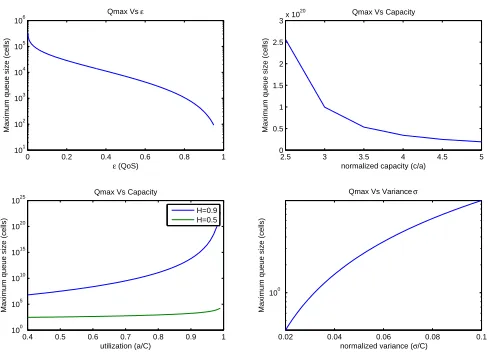
The graphical interpretation of the expected qmax is shown in Figure 2.4. The intuitions we
get are:
• The smaller the buffer (i.e.,qmax), the bigger the probabilityǫof having an overflow (see
upper left graph).
• As the service rate/capacity C increases we can provide the same QoS (i.e., ǫ) with even less buffer size (i.e.,qmax) (see upper right graph).
• As the arrival traffic increases we need a bigger buffer (i.e.,qmax) in order to accommodate
the incoming traffic given the probability of loss ǫ(see graphs in the bottom).
We have a SLA violation if at given traffic conditions ¯α, σ andH, the expected delay Dmax
for the agreed QoS ǫis greater than the delay boundd.
2.3.2 Convex optimization
Putting the revenue and cost components together, the provider’s profit problem becomes:
max φ {
k
X
i=1
piφiC− k
X
i=1
0 0.2 0.4 0.6 0.8 1
101
102
103
104
105
106
ε (QoS)
Maximum queue size (cells)
Qmax Vs ε
2.5 3 3.5 4 4.5 5
0 0.5 1 1.5 2 2.5
3x 10
20
normalized capacity (c/a)
Maximum queue size (cells)
Qmax Vs Capacity
0.4 0.5 0.6 0.7 0.8 0.9 1
100
105
1010
1015
1020
1025
utilization (a/C)
Maximum queue size (cells)
Qmax Vs Capacity H=0.9 H=0.5
0.02 0.04 0.06 0.08 0.1
100
normalized variance (σ/C)
Maximum queue size (cells)
Qmax Vs Variance σ
Figure 2.4: Graphical interpretation of the probabilistic queue boundqmax
subject to the feasibility constraints previously described, plus the constraints φi > α¯i, i =
1. . . k. The last constraint, φi >α¯i, should always stand true due to the fact that whenever φi ≤α¯i we have P r[Q(t) > qmax] = 1. This implies that we are in an unstable case and the
queue would never be able to accommodate the incoming traffic. This constraint is introduced in order to impede the network from operating in this undesirable (from a QoS perspective) regime.
In the over-provisioned case (i.e., when Piα¯i ≤ 1), a unique solution exists, due to the
convex nature of the problem, as argued next.
Proposition 2.3.1. Maximizing the objective function (2.8) is a convex optimization problem.
Proof. It is sufficient to show that we are maximizing a concave function over a convex constraint
set.
Starting from the constraint set we observe that we have a set of affine functions. Affine functions are convex. Moreover, the intersection of convex sets is convex. Thus, the constraint set is convex.
Now, we have to prove that the utility function is concave. To achieve that we will use some well known convex preserving operations. To start with, we show that the second derivative of
Di(φi) =A
(φi−α¯)H/(H−1) φi
, whereA= (kσ)1/(1−H)HH/(1−H)(1−H)>0
∂Di ∂φi
=A (
H
H−1
(φi−α¯)1/(H−1)
φi −
(φi−α¯)H/(H−1) φ2
i
)
∂2Di ∂φ2
i
=A (
2H
1−H
(φi−α¯)1/(H−1) φ2
i
+ H
(H−1)2
(φi−α¯)(2−H)/(H−1) φi
+2(φi−α¯)
H/(H−1)
φ3
i
)
From the above equations and the fact that the Hurst parameter H ∈[0.5,1) we conclude that Di′′(φi) >0 in the feasibility set. Thus, Di(φi) is convex on R. The cost function ci(Di)
is an exponential function which is convex in the feasibility set and nondecreasing. We know that if a function h is convex and nondecreasing and functiong is convex then f =h(g(x)) is convex. Therefore,ci(Di(φi)) is convex onR as a composition of a convex and nondecreasing
function with a convex function.
In addition,g(φ) =PKi=1ci(φi) is convex on RK because its Hessian is positive definite. Its
Hessian is shown below and as we can see all the diagonal elements of the Hessian are positive and hence the Hessian is positive definite.
∇2g=
∂2D 1 ∂φ2
1 0 . . . 0
0 ∂2D2 ∂φ2
2 . . . 0
..
. 0 . .. 0
0 . . . 0 ∂2DK
∂φ2 K
Hence,−g(φ) is concave. PpiφiCis also concave and thus the sum of two concave functions
is concave. Thus, we are dealing with a concave utility function and our problem is a convex optimization problem.
The optimal solution can then be found using Newton-type algorithms. Notice that we are dealing with a constrained optimization problem, which implies that appropriate methods need to be considered (e.g., a penalty or barrier function to relax the constraints [56]). In addition, we can take advantage of the Karush-Kuhn-Tucker (KKT) conditions that are necessary and sufficient for primal-dual optimality of a convex optimization problem. The primal problem is translated to an equivalent, but easier to solve dual problem. The primal problem has solution
lies on the hyperplanePki=1φi = 1. The proof and the KKT conditions are given next: k
X
i=1
φ∗i −1≤0 (2.9a)
−φ∗i + ¯αi <0,∀i∈ {1. . . k} (2.9b)
λ∗i ≥0,∀i∈ {1. . . k} (2.9c)
λ∗1(
k
X
i=1
φ∗i −1) = 0 (2.9d)
λ∗i+1(−φ∗i + ¯αi) = 0,∀i∈ {1. . . k} (2.9e) ∂π(φ)
∂φi −
(λ∗1−λ∗i+1) = 0,∀i∈ {1. . . k} (2.9f)
From (2.9f) and since ∂π∂φ(φ)
i >0 we get thatλ
∗
1−λ∗i+1 >0. From the secondcomplementary
slackness condition (2.9e), we obtain λ∗i+1 = 0 since the constraint −φ∗i + ¯αi < 0 always
holds. Hence, we conclude thatλ∗1 >0, which together with the other complementary slackness condition (2.9d) gives thatPki=1φ∗
i −1 = 0.
The optimal solution is found using a sequential quadratic programming (SQP) algorithm which is the state of the art for solving constrained optimization problems [56]. The algorithm’s performance allows MBORA to accommodate a large number of service classes.
2.4
Online Traffic Measurement and Traffic Monitoring
Next, we discuss the measurement module, whose main responsibilities include on-line traffic measurements and traffic monitoring. Traffic changes are monitored using the EWMA control chart and when traffic changes of any service class are detected, an out-of-control signal is triggered. Then, a process for on-line traffic estimation is initiated and when it is completed the new traffic parameters are passed to the optimization module.
As previously mentioned, it is assumed that traffic is governed by a self-similar process. Specifically, traffic is modeled using the fractional Brownian motion (fBm) process and thus estimation of the Hurst parameter H that captures the degree of LRD is crucial. For this purpose, we have selected to employ the LASS tool [57], which has a powerful set of estimation techniques for LRD data, based on wavelets (for a comprehensive review of the methodology see [57]).
intensities (i.e., mean rate αi) are altered. This makes our MBORA system computationally
less expensive than a system that has to continually solve the optimization problem even when traffic parameters remain unchanged. At this point, we need to clarify that traffic parameters
Hiandσiare not assumed to remain fixed; they can vary asαidoes. However, we do not apply
the EWMA control scheme on them. We believe thatαi changes more frequently than the other
two parameters and thus we just monitorαi. Nonetheless, when we redo traffic measurements, Hi and σi are also recalculated and any possible changes on their values will be captured.
For implementation purposes, time is divided into non-overlapping intervals (tn, tn+1),n= 0,1,2, . . .of duration ∆. The measurement module counts the number of packets from each class that arrive during each interval (eventually, this sequence of points consists a fractional Gaussian noise (FGN) process) in order to obtain the sequence of traffic intensities{αˆi(1),αˆi(2), . . .}for
each classi. The EWMA statistic for that class would then be:
¯
αi(n+ 1) =β×αˆi(n) + (1−β)×α¯i(n) (2.10)
where ¯αi(n+ 1) is the one-step-ahead prediction of ˆαi(n+ 1) and 0 < β ≤ 1 represents the
weight that the most recent estimation is assigned (see [46], [45]). The initial prediction, i.e. ˆ
αi(0), should be set equal to the mean rate αi (known as the target value). Thus, the meanαi
and variance σ2
i of each FGN sequence should be estimated a priori.
Moreover, based on the current traffic statistics (i.e.,αi andσ2i) we can compute the control
limits of an EWMA chart for traffic class i. The lower and upper control limits are given as:
LCL/U CL=αi±cσi
s β
2−β (2.11)
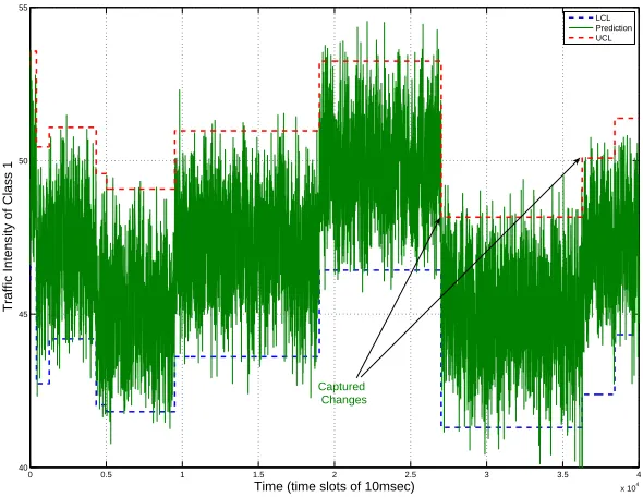
where parameter c > 0 is a tuning variable that combined with parameter β can set the sensitivity level that the provider needs to accomplish. A more sensitive EWMA control chart would capture more subtle traffic shifts; however, it would also give more frequent out-of-control signals even when traffic has not really changed (false positive errors) [45]. Hence, the provider needs to consider the trade-off between accuracy and computational effort. An out-of-control signal is generated at time slotn when ¯αi(n)> U CLor ¯αi(n)< LCL. An example of EWMA
chart is depicted in Figure 2.5.
0 0.5 1 1.5 2 2.5 3 3.5 4
x 104
40 45 50 55
Time (time slots of 10msec)
Traffic Intensity of Class 1
LCL Prediction UCL
Captured Changes
Figure 2.5: The Exponentially Weighted Moving Average Chart.
module, we must receive two out-of-control signals from the EWMA traffic monitor.
2.5
Performance Evaluation
2.5.1 Sensitivity to Model Parameters
In this section, the goal is to investigate how the utility function, π(φ~), and the resource allocation vector,φ~, respond to changes of various parameters, including the mean arrival rate
¯
αi, the pricepi, the delay thresholddi and the Hurst parameterHi. We start our analysis with
a simple system of two service classes and then we continue with a larger one of six service classes.
A system comprised of two service classes
In this case, the corresponding utility function is given by:
π(φ1, φ2) =p1φ1C+p2φ2C−b1D1(φ1)e10(D1(φ1)−d1)−b2D2(φ2)e10(D2(φ2)−d2) (2.12)
whereDi(φi) = (φi−α¯i)
Hi
Hi−1(kσi)1−1HiH
Hi
1−Hi
i (1−Hi)
φi , i= 1,2.
Hence, we have to solve the optimization problem:
max
φ π(φ1, φ2) subject to φ1+φ2 = 1,φ1 >α¯1 and φ2 >α¯2.
(2.13)
The parameters of the profit function used in this study are shown in Table 2.1. Note that the traffic parameters ¯αi and σi are normalized to the capacity C. The function’s concavity
over both arguments is shown graphically in Figure 2.6a. In Figure 2.6b, we view the utility function with respect to the first argument by substitutingφ2 with 1−φ1.
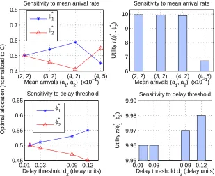
Figure 2.7 (upper panels) demonstrates the optimal solution when the arrival rate varies. It can be observed that in the equal arrival rates case the resources are equally shared. On the other hand, if a class brings more traffic load, then it is assigned a larger portion of the resources. Moreover, notice that as the system becomes more stressed, the overall profit of the provider decreases substantially; this is because a higher utilization of the system implies longer queue delays and, therefore, the value of the cost function increases, a fact that is compatible with the analytic derivation that shows that ∂π/∂α¯i <0.
In Figure 2.7 (lower part) we examine the sensitivity of our model with respect to the delay thresholddi. Notice that as the threshold increases (i.e., the QoS requirement is relaxed), the
profitπof the provider also increases, which is due to the fact that∂π/∂di =biβiDieβi(Di−di)>
0. It is also worth noting that the class with stricter QoS requirements is allocated more resources (class-1 in this case).
Table 2.1: Parameters of each service class i(i= 1,2)
Parameter pi bi di QoS (=ǫ) α¯i σi Hi
price unit M bps
price unit
msec delay unit
Class−i 1 0.1 0.01 10−6 0.2 0.01 0.7
0.2 0.3 0.4 0.5 0.6 0.2 0.3 0.4 0.5 0.6 0.7 4 6 8 10 12 14 φ1 X: 0.5 Y: 0.5 Z: 9.957
Utility function as a function of φ1, φ2
φ2
(a) Utility as a function ofφ1,φ2.
0.3 0.4 0.5 0.6 0.7 9 9.1 9.2 9.3 9.4 9.5 9.6 9.7 9.8 9.9 10 φ1 Utility Function
Utility function as a function of φ1
(b) Utility as a function ofφ1.
Figure 2.6: Concavity of our utility function
(2, 2) (3, 2) (4, 2) (4, 5)
0.4 0.5 0.6 0.7 0.8
Mean arrivals (a
1, a2) (x10 −1)
Optimal allocation (normalized to C)
Sensitivity to mean arrival rate
φ* 1
φ* 2
(2, 2) (3, 2) (4, 2) (4, 5)
6 7 8 9 10
Mean arrivals (a
1, a2) (x10 −1)
Utility
π
(
φ
* , 1
φ
* ) 2
Sensitivity to mean arrival rate
0.03
0.01 0.09 0.12
0.45 0.5 0.55 0.6 0.65
Delay threshold d
2 (delay units)
φ1*
φ2*
0.03
0.01 0.09 0.12
9.95 9.96 9.97 9.98 9.99
Sensitivity to delay threshold
Delay threshold d
2 (delay units)
Utility π ( φ 1 * , φ 2 * ) Sensitivity to delay threshold
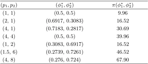
Table 2.2: Changing the pricing factor pi. (p1, p2) (φ∗1, φ∗2) π(φ∗1, φ∗2)
(1, 1) (0.5, 0.5) 9.96
(2, 1) (0.6917, 0.3083) 16.52 (4, 1) (0.7183, 0.2817) 30.69
(4, 4) (0.5, 0.5) 39.96
(1, 2) (0.3083, 0.6917) 16.52 (1.5, 6) (0.2739, 0.7261) 46.52 (4, 8) (0.276, 0.724) 67.90
Table 2.1). Again, with equal prices we obtain equal allocations, while the allocation of resources exhibits a strong sensitivity to the price ratiop1/p2.
Table 2.3: Sensitivity to Hurst parameterHi. HurstHi |∆Hi| δHi×100% Allocationφi |∆φi| δφi×100%
0.8 0 0 0.5 0 0
0.78 0.02 2.5 0.4947 0.0053 1.06 0.75 0.05 6.25 0.488 0.012 2.4
0.7 0.1 12.5 0.4796 0.0204 4.08 0.65 0.15 18.75 0.4737 0.0263 5.26 0.82 0.02 2.5 0.5062 0.0062 1.24
Moreover, Table 2.3 exhibits the sensitivity of the allocation with respect to the Hurst parameter (we denote by|∆x|the absolute error and byδxthe relative error on the measurement
for variablex). We observe that the allocation is not significantly affected by minor variations, ∆Hi, of the Hurst parameter. Hence, our model is robust to reasonable miscalculations of the Hurst parameter H.
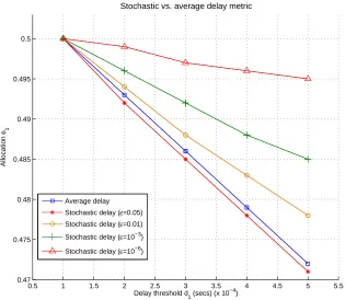
In Figure 2.8, we compare MBORA with a system that employs an average delay metric. Specifically, it uses the average delay of an M/M/1 queue which is given by D= µ−1λ, where
λ is the Poisson arrival rate and 1/µ the mean service time. We assume that λ = ¯αiC/L
and µ = φiC/L, where L is the mean message length (we set L = 50 bytes). The modeling
parameters of the experiment are as follows (for i = {1,2}): ¯αi = 0.4, σi = 0.01, Hi = 0.8, βi = 104, capacity C = 10 Mbps and delay threshold for class-2 isd2 = 100 usec. Figure 2.8 shows that the stochastic delay metric offers a greater flexibility to the provider. The QoS parameter, ǫi, serves as a tuning factor of the allocated resources; the stricter the desired QoS
0.5 1 1.5 2 2.5 3 3.5 4 4.5 5 5.5 0.47
0.475 0.48 0.485 0.49 0.495 0.5
Delay threshold d
1 (secs) (x 10 −4)
Allocation
φ1
Stochastic vs. average delay metric
Average delay
Stochastic delay (ε=0.05)
Stochastic delay (ε=0.01)
Stochastic delay (ε=10−3)
Stochastic delay (ε=10−6)
Figure 2.8: Allocation using an average delay metric versus the allocation using our stochastic delay metric.
is sensitive to the choice of ǫi whereas a system that depends on average delays provisions a
fixed, indisputable and not very reliable allocation.
A system comprised of six service classes
Table 2.4: Sensitivity to mean arrival rate ¯αi.
( ¯α1, ¯α2, ¯α3, ¯α4, ¯α5, ¯α6) (φ1,φ2,φ3,φ4,φ5,φ6) π(φ~∗) 0.10, 0.10, 0.10,0.10, 0.10, 0.10 0.167, 0.167, 0.167, 0.167, 0.167, 0.167 83.74 0.11 , 0.10, 0.10, 0.10, 0.10, 0.10 0.174, 0.165, 0.165, 0.165, 0.165, 0.165 82.50 0.12 , 0.11, 0.10, 0.10, 0.10,0.10 0.180, 0.171, 0.162, 0.162, 0.162, 0.162 79.52 0.13 , 0.12, 0.11, 0.10, 0.10 ,0.10 0.185, 0.176, 0.167, 0.158, 0.158, 0.158 73.42 0.13, 0.12, 0.11, 0.11 ,0.10 ,0.10 0.183, 0.174, 0.165, 0.165, 0.156, 0.156 70.79 0.13, 0.12, 0.11, 0.11, 0.12, 0.13 0.176, 0.167, 0.158, 0.158, 0.167, 0.176 49.09 0.13, 0.12, 0.11, 0.12,0.13, 0.14 0.171, 0.162, 0.153, 0.162, 0.171, 0.180 21.73 0.10, 0.11, 0.12, 0.13, 0.14, 0.15 0.144, 0.153, 0.162, 0.171, 0.180, 0.190 21.18 0.10, 0.11, 0.12, 0.13, 0.14, 0.20 0.136, 0.145, 0.154, 0.163, 0.173 , 0.229 -122.60
Table 2.5: Sensitivity to pricing parameterpi.
(p1,p2,p3,p4,p5,p6) (φ1,φ2,φ3,φ4,φ5,φ6) π(φ~∗) 1.00,1.00, 1.00, 1.00 , 1.00, 1.00 0.167, 0.167, 0.167, 0.167, 0.167, 0.167 83.74 2.00, 1.00, 1.00, 1.00, 1.00, 1.00 0.179, 0.164, 0.164, 0.164, 0.164, 0.164 100.94 3.00, 2.00, 1.00, 1.00, 1.00, 1.00 0.193, 0.167, 0.160, 0.160, 0.160, 0.160 136.09 4.00, 3.00, 2.00, 1.00, 1.00, 1.00 0.202, 0.168, 0.161, 0.156, 0.156, 0.156 188.66 5.00, 4.00, 3.00, 2.00, 1.00, 1.00 0.206, 0.169, 0.161, 0.156, 0.154 , 0.154 257.66 6.00, 5.00, 4.00, 3.00, 2.00, 1.00 0.208, 0.169, 0.161, 0.157, 0.154, 0.152 342.40 6.00, 5.00, 4.00 , 3.00, 2.00, 6.00 0.183, 0.166, 0.159, 0.155, 0.153, 0.183 422.80 6.00, 5.00, 4.00, 3.00, 2.00, 7.00 0.169, 0.161, 0.157, 0.154, 0.152, 0.208 442.40 6.00, 5.00, 4.00, 3.00, 8.00, 7.00 0.161, 0.157, 0.154, 0.152, 0.208, 0.169 542.40
In the latter table, we view that the allotment of resources is done according to the priority (e.g. price) of each service. The results of both tables are in agreement with our conclusions of the previous subsection regarding the two service class system. Further, the results indicate that the optimization module is scalable and robust to large systems.
2.5.2 Assessing the dynamic behavior of MBORA
Table 2.6: Responsiveness to traffic changes. Evaluating the dynamic behavior of MBORA.
Time slots Actual Traffic Monitoring, Estimation Optimization
×105 ( ¯α1,α¯2) ( ¯α1,α¯2) (H1, H2) (φ1, φ2) Utilityπ 0−0.4 0.14, 0.22 0.14, 0.22 0.58, 0.57 0.47, 0.53 8.04 0.4−0.9 0.20, 0.30 0.20, 0.30 0.57, 0.57 0.46, 0.54 7.22 0.9−1.2 0.16, 0.22 0.16, 0.22 0.62, 0.63 0.48, 0.52 8.88 1.2−1.6 0.19, 0.20 0.19, 0.20 0.60, 0.62 0.50, 0.50 8.65 1.6−2.6 0.26, 0.18 0.26, 0.18 0.60, 0.61 0.53, 0.47 8.32 2.6−3 0.14, 0.22 0.14, 0.22 0.59, 0.62 0.48, 0.52 8.6
3−4 0.26, 0.18 0.26, 0.18 0.57, 0.63 0.55, 0.45 8.25 4−10 0.19, 0.21 0.19, 0.21 0.60, 0.58 0.48, 0.52 8.17
that the mean and the variance are normalized to the capacity Cof the network element). The purpose of this experiment is twofold: first, we evaluate if EWMA correctly captures the traffic changes and second we compare the total utility and computation time of both systems (i.e., MBORA vs. naive) to see if traffic prediction and monitoring enhances the performance of our system. Intuition suggests that MBORA will be computationally more efficient than the naive system, but less accurate. Before we proceed, we give the definition of the total utility achieved by the MBORA system for a period of T time units:
ˆ
U∗= 1
T KT+1
X
i=1
π(φ~∗(i))(t
i−ti−1) (2.14)
where KT is the number of traffic changes that took place, ti is the time instance that change ihappened, andπ(φ~∗(i)) is thelocal utility in the time period between the change i−1 andi.
For example, in Table 2.6 we observe thatKT = 7 changes.
−1 0 1 2 3 4 5 6 7 8 9 5
5.5 6 6.5 7 7.5 8 8.5 9 9.5
Time slot (x 105)
Local utility (utility units)
MBORA vs. Oracle−I: Assessing the sensitivity of EWMA on traffic changes
Oracle−I
MBORA
0 1 2 3 4 5 6 7 8 9 0
10 20 30 40 50 60 70 80 90 100
Time slot (x 105)
Mean traffic load
αi
(i=1,2) (packets/slot)
Mean traffic load αi for both classes
Shifted by
E(τ) + T
H
(on average)
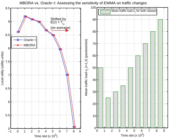
Figure 2.9: MBORA vs. Oracle-I: evaluation of EWMA’s sensitivity to traffic shifts (see dis-cussion in subsection 2.5.3)
2.5.3 Evaluation of traffic monitoring and estimation
This section discusses a comparison between the proposed MBORA system and two idealized systems that behave asoracles. The first oracle system (referred to as Oracle-I) knows exactly when traffic changes occur. Thus, a comparison with Oracle-I help us assert whether MBORA’s EWMA scheme accurately captures traffic shifts. The second oracle system (called Oracle-II) is consistently aware of the triplet (¯α, σ, H) of the incoming traffic. This comparison assists us evaluate the accuracy of the model’s traffic estimator.
Performance analysis of EWMA
3 4 5 6 7 8 9 10 11 12 7.2
7.4 7.6 7.8 8 8.2 8.4 8.6
Parameter c
Total utility (utility units)
Sensitivity to parameter c
ORACLE MBORA
True Utility
Utility Deficit
Figure 2.10: Sensitivity of EWMA to parameter c. The Oracle-I system yields a precise total utility whereas MBORA has a utility deficit according to the value of c.
one of Oracle-I. MBORA returned a total utility of 7.35 utility units whereas Oracle-I gave a total utility of 7.28. The utility deficit is 0.07 which translates to only ∼1%. This is because we have judiciously chosen the EWMA parameters, β and c, so as to yield a sensitive enough monitoring system that would capture most (if not all) traffic alterations. The disadvantage of this approach is that it increases the number of false positive out-of-control signals. This causes the optimization problem to be solved even when there is no real traffic modification and, therefore, computing resources are wasted gratuitously. Thus, the network architect should consider the important trade-off among accuracy and performance. This trade-off can be tuned by the choice of the EWMA parameters,β andc. These parameters administer theaverage
run-length (symbolized as E(τ)) of EWMA which is defined as the mean number of slots required
to capture the traffic shift. Lucas et al.[45] provide tables for obtaining E(τ).
Insights into the sensitivity of the EWMA system with respect to parameter c is provided by examining Figure 2.10. Note that as parameter c increases, the utility deficit increases as well, because EWMA becomes less sensitive to traffic changes. On the other hand, the number of false positive signals is reduced.
larger bound denotes a system that generates fewer false positive out-of-control signals; on the other hand, some traffic shifts may not be detected and MBORA’s correctness is deteriorated. To apply Proposition (2.5.1) for a period of T time slots we need to know: (a) the average run-length,E(τ), for the given choice ofβ and c, (b)TH, representing the number of time slots
required by MBORA’s traffic estimator to measure the incoming load, (c) the amount of traffic alterations during period T, represented by KT,and (d) the maximum difference between two
consecutive local utilities. For the scenario of traffic shifts of Figure 2.10 the utility deficit bound is calculated to be ∆ ≤ |7.01−5.06|×9×810×(25 .5+10000) = 0.09 utility units. Indeed, the real
deficit between MBORA and Oracle-I is 0.07 which is below our calculated utility bound. The deficit bound is given by the proposition that follows.
Proposition 2.5.1. The use of EWMA introduces a utility deficit because traffic changes cannot be captured immediately. We can achieve a bound on that deficit by adhering to the following assumptions:
• Let S={1,2, . . . , KT(n)}be the index set of traffic changes in the period [0, nTs]wheren
is the time slot number, Ts is the duration of the time slot and T =nTs is the total time
length that average utility is calculated (see Figure 2.11). We assume thatKT(n) =o(n),
i.e. KnTT(n)
s is bounded asn→ ∞.
• All traffic changes are captured by EWMA control scheme.
• There is an Oracle system that knows exactly when traffic shifts occur. The average
optimum utility of such system is given by:
U∗ = 1
T
RT
0 π(φ~∗(t))dt= 1
T
PKT+1
i=1
Rti
ti−1π(
~
φ∗(i))dt where t
i is the beginning of traffic shift
i.
• The MBORA system has an average utility:
ˆ
U∗ = 1
T
RT
0 π(φ~∗(t))dt = T1
PKT+1
i=1
Rˆti ˆ
ti−1π(
~
φ∗(i))dt where ˆti =ti+τi+TH,τi is a random
variable indicating the time length needed for EWMA to capture traffic shift i and TH is
the number of slots needed to obtain an accurate estimation of the new traffic parameters.
The upper bound ∆ is given by:
∆ =||Uˆ∗−U∗
|| ≤max
i∈S ||π( ~
φ∗(i))−π(φ~∗(i+ 1))||KT
T (E(τ) +TH) (2.15)
whereE(τ) is the average run length for a particular parameter pair(β, c)of the EWMA control