Selection Theory for Marker-Assisted Backcrossing
Matthias Frisch and Albrecht E. Melchinger
1Institute of Plant Breeding, Seed Science and Population Genetics, University of Hohenheim, 70593 Stuttgart, Germany
Manuscript received August 27, 2004 Accepted for publication February 21, 2005
ABSTRACT
Marker-assisted backcrossing is routinely applied in breeding programs for gene introgression. While selection theory is the most important tool for the design of breeding programs for improvement of quantitative characters, no general selection theory is available for marker-assisted backcrossing. In this treatise, we develop a theory for marker-assisted selection for the proportion of the genome originating from the recurrent parent in a backcross program, carried out after preselection for the target gene(s). Our objectives were to (i) predict response to selection and (ii) give criteria for selecting the most promising backcross individuals for further backcrossing or selfing. Prediction of response to selection is based on the marker linkage map and the marker genotype of the parent(s) of the backcross population. In comparison to standard normal distribution selection theory, the main advantage of our approach is that it considers the reduction of the variance in the donor genome proportion due to selection. The developed selection criteria take into account the marker genotype of the candidates and consider whether these will be used for selfing or backcrossing. Prediction of response to selection is illustrated for model genomes of maize and sugar beet. Selection of promising individuals is illustrated with experimental data from sugar beet. The presented approach can assist geneticists and breeders in the efficient design of gene introgression programs.
M
ARKER-ASSISTED backcrossing is routinely ap- the expected donor genome proportion in generation plied for gene introgression in plant and animal BCn is 1/2n⫹1. In backcrossing with selection for the breeding. Its efficiency depends on the experimental presence of a target gene,StamandZeven(1981) de-design, most notably on the marker density and posi- rived the expected donor genome proportion on the tion, population size, and selection strategy. Gene intro- carrier chromosome of the target gene, extending ear-gression programs are commonly designed using guide- lier results ofBartlettandHaldane(1935),Fisher lines taken from studies focusing on only one of these (1949), andHanson(1959) on the expected length of factors (e.g.,Hospitalet al.1992;Visscher1996;Hos- the donor chromosome segment attached to the target pitalandCharcosset1997;Frischet al.1999a,b). In gene. Their results were extended to a chromosome breeding for quantitative traits, prediction of response carrying the target gene and the recurrent parent alleles to selection with classical selection theory is by far the at two flanking markers (Hospitalet al.1992) and to most important tool for the design and optimization of a chromosome carrying several target genes (Ribaut breeding programs (Bernardo 2002). Adopting a se- et al.2002).lection theory approach to predict response to marker- Hill (1993) derived the variance of the donor ge-assisted selection for the genetic background of the nome proportion in an unselected backcross popula-recurrent parent promises to combine several of the tion, whereasRibautet al.(2002) deduced this variance factors determining the efficiency of a gene introgres- for chromosomes carrying one or several target genes. sion program into one criterion. The covariance of the donor genome proportion across In classical selection theory, the expectation, genetic a chromosome and the proportion of donor alleles at variance, and heritability of the target trait are required, markers in backcrossing was given byVisscher(1996). as well as the covariance between the target trait and In their derivations, these authors assumed that the the selection criterion in the case of indirect selection donor genome proportion of different individuals in a (Bernardo 2002). In backcrossing without selection, backcross generation is stochastically independent. This applies to large BCnpopulations only (a) in the absence of selection in all generations BCs(1ⱕsⱕn) and (b) if each BCn⫺1(n⬎1) individual has maximally one BCn
This article is dedicated to Professor Dr. H. F. Utz on the occasion
of his 65th birthday. His teaching of selection theory was most instru- progeny (comparable to the single-seed descent method mental to the authors.
in recurrent selfing).Visscher(1999) showed with
sim-1Corresponding author:Institute of Plant Breeding, Seed Science,
ulations that the variance of the donor genome
propor-and Population Genetics, University of Hohenheim, 70593 Stuttgart,
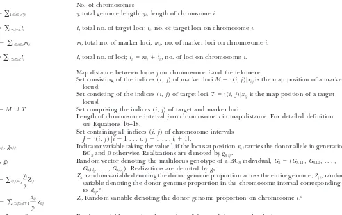
TABLE 1 Notation
c No. of chromosomes
y⫽
兺
1ⱕiⱕcyi y, total genome length;yi, length of chromsomei.t⫽
兺
1ⱕiⱕcti t, total no. of target loci;ti, no. of target loci on chromosomei.m⫽
兺
1ⱕiⱕcmi m, total no. of marker loci;mi, no. of marker loci on chromosomei.l⫽
兺
1ⱕiⱕcli l, total no. of loci;li⫽mi⫹ti, no. of loci on chromosomei.xi,j Map distance between locusjon chromosomeiand the telomere.
M Set consisting of the indices (i,j) of marker lociM⫽{(i,j)|xi,jis the map position of a marker locus}.
T Set consisting of the indices (i,j) of target lociT⫽{(i,j)|xi,jis the map position of a target locus}.
L⫽M傼T Set comprising the indices (i,j) of target and marker loci .
di,j Length of chromosome intervaljon chromosomeiin map distance. For detailed definition see Equations 16–18.
J Set containing all indices (i,j) of chromosome intervals
J⫽{(i,j) |i⫽1 . . .c,j⫽1 . . .li⫹1}.
Gn,i,j,gn,i,j Indicator variable taking the value 1 if the locus at positionxi,jcarries the donor allele in generation BCnand 0 otherwise. Realizations are denoted bygn,i,j.
Gn,gn Random vector denoting the multilocus genotype of a BCnindividual,Gn⫽(Gn,1,1,Gn,1,2, . . . , Gn,1,l1, . . . ,Gn,c,lc). Realizations are denoted bygn.
Zn, random variable denoting the donor genome proportion across the entire genome;Zi,j, random Z⫽
兺
(i,j)僆Jyi
yZi,j variable denoting the donor genome proportion in the chromosome interval corresponding
todi,j.a
Zi, Random variable denoting the donor genome proportion on chromosomei.a Zi⫽
兺
1ⱕjⱕli⫹1di,j yi
Zi,j
B⫽
兺
(i,j)僆MGn,i,j Random variable counting the number of donor alleles at marker loci.aRandom variablesZ,Z
i, andZi,jrefer to the homologous chromosomes originating from the nonrecurrent parent.
lection is significantly smaller than that in unselected map of the target gene(s) and markers, and (c) the marker genotype of the individuals used as nonrecur-populations of stochastically independent individuals.
Hillelet al.(1990) andMarkelet al.(1997) employed rent parents for generating backcross generations BCs (sⱕn).
the binomial distribution to describe the number of homozygous chromosome segments in backcrossing. However, Visscher(1999) demonstrated with
simula-THEORY tions that the assumption of binomially distributed
chro-mosome segments results in an unrealistic prediction For all derivations we assume absence of interference of the number of generations required for a marker- in crossover formation such that the recombination fre-assisted backcross program. Hence, the expectations, quencyrand map distancedare related byHaldane’s variances, and covariances are known for backcrossing (1919) mapping functionr(d)⫽(1⫺e⫺2d)/2. An over-without selection, but these approximations are of lim- view of the notation used throughout this treatise is ited use as a foundation of a general selection theory given in Table 1.
for marker-assisted backcrossing. In the following we derive (1) the expected donor The objective of this study was to develop a theoretical genome proportion of a backcross individual condi-framework for marker-assisted selection for the genetic tional on its multilocus genotypegnat marker and target background of the recurrent parent in a backcross pro- loci, (2) the expected donor genome proportion of a gram to (i) predict response to selection and (ii) give backcross population generated by backcrossing an indi-criteria for selecting the most promising backcross indi- vidual with multilocus genotypegnto the recurrent par-viduals for further backcrossing or selfing. Our approach ent, and (3) the expected donor genome proportion deals with selection in generation n of the backcross of the wth-best individual of a backcross population program, taking into account (a) preselection for the of sizeugenerated by backcrossing an individual with
Probability of multilocus genotypes: We derive the Selection of individuals with a low number of donor alleles:We determine the distribution of donor alleles probability that a BCnindividual has multilocus
geno-typegnunder the condition that its nonrecurrent parent in the individual carrying (1) all target genes and (2) the
wsmallest number of donor alleles among all carriers of has multilocus genotypegn⫺1. Let
the target genes (subsequently referred to as thewth
I⫽{(i,j)|(i,j)僆 L,gn⫺1,i,j⫽ 1 } (1)
best individual).
Assume thatvout ofuindividuals of a backcross family denote the set of indices, for which the locus at position
carry all target genes. Then, the distribution of donor
xi,jwas heterozygous in the nonrecurrent parent in
gen-alleles in thewth best individual among thev carriers eration BCn⫺1(F1⫽BC0). The elements ofIare ordered
of the target gene is described by thewth order statistic according to
of v independent random variables with distribution (i⬘,j⬘)≺(i,j) iff (i⬘ ⬍i) or [(i⬘ ⫽i) and (j⬘ ⬍j)]. functionF(b). Its distribution function is
(2)
Fw:v(b)⫽
兺
vi⫽w
冢
v i
冣
F(b)w[1⫺F(b)]v⫺w (11) The conditional probability that the BCnindividual has
the multilocus marker genotypegnis
(David 1981). Weighing with the probability that
ex-P(Gn⫽gn|gn⫺1)⫽
兿
(i,j)僆I{␦i,jr*i,j ⫹ (1⫺ ␦i,j)(1⫺r*i,j)}, actlyvindividuals carry the target gene yields the distri-bution function of donor alleles in thewth best carrier (3)
of all target genes in a BCnfamily of sizeu, where
Hw,u(b)⫽
兺
0ⱕvⱕuP(V⫽v)Fw:v(b) (12) ␦i,j⫽
冦
gn,i,j forj⫽1
|gn,i,j⫺gn,k,l| otherwise (4) with
with
P(V⫽ v)⫽
冢
uv
冣
pv(1⫺p)u⫺v, (13) (k,l)⫽ max{(i⬘,j⬘)|(i⬘,j⬘)僆 I, (i⬘,j⬘)≺(i,j)} (5)
where the probability p that an individual carries all and
target genes is
r*i,j ⫽
冦
1⁄2 forj⫽ 1
r(xi,j⫺ xk,l) otherwise.
(6) p⫽
兿
(i,j)僆T
(1 ⫺r*i,j) (14)
andr*i,j is calculated analogously to Equations 5 and 6 Distribution of donor alleles at markers: Consider a
but replacingIwith T. BCn family of size u, generated by backcrossing one
The probability that thewth best individual carriesb
BCn⫺1individual to the recurrent parent. Let
donor alleles is
B⫽
兺
(i,j)僆MGn,i,j (7)
hw,u(b)⫽
冦
Hw,u(b) forb⫽0
Hw,u(b)⫺Hw,u(b⫺1) forb ⬎0.
(15) denote the number of donor alleles at the marker loci
of a BCnindividual. The probability that an individual
Distribution of the donor genome proportion:In the that carries all target genes is heterozygous at exactlyb
following, we investigate the homologous chromosomes loci is
of backcross individuals that originate from the nonre-current parent. We divide the chromosomes into
non-f(b)⫽ Pt(B⫽b)⫽
兺
gn僆Ᏻn,t,bP(Gn⫽ gn|gn⫺1)
兺
gn僆Ᏻn,tP(Gn⫽ gn|gn⫺1), (8)
overlapping intervals,
where
(ai,j,bi,j)⫽
冦
(0,xi,j) forj⫽1 (xi,j⫺1,xi,j) for 1⬍jⱕli (xi,li,yi) forj⫽li⫹1
(16)
Ᏻn,t⫽
冦
gn|t⫽兺
(i,j)僆Tgn,i,j
冧
(9)with length denotes the set of all multilocus marker genotypes
car-rying all target genes and d
i,j⫽bi,j⫺ai,j (17)
Ᏻn,t,b⫽
冦
gn|gn僆Ᏻn,t,b⫽兺
(i,j)僆Mgn,i,j
冧
(10) for each(i,j)僆 J⫽ {(i,j)|i⫽1 . . .c,j⫽ 1 . . .li⫹ 1 }. (18) denotes the set of all multilocus marker genotypes
carry-ing all target genes and the donor allele at exactlybmarker Consider a BCnindividual with genotypegnof which the genotype of the nonrecurrent parent in generations loci. The respective distribution function is F(b) ⫽ Pt
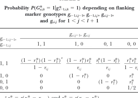
TABLE 2 mologous chromosomes originating from the nonrecur-rent panonrecur-rent of a BCnindividual with genotypegncan then
ProbabilityP(G*s,i,k⫽1|g*s⫺1,i,k⫽1) depending on flanking
be determined as
marker genotypesgs⫺1,i,j⫺1,gs⫺1,i,j,gs,i,j⫺1,
andgs,i,jfor 1⬍j⬍l⫹1
z(gn)⫽
兺
(i,j)僆Jdi,j
yE(Zi,j). (24) gs,i,j⫺1,gs,i,j
gs⫺1,i,j⫺1,
gs⫺1,i,j 1, 1 1, 0 0, 1 0, 0 Response to selection: We define response to selec-tion R as the difference between the expected donor genome proportionin the selected fraction of a BCn 1, 1 (1⫺r*1)(1⫺r*2)
1⫺ri,j a
(1⫺r*1)r*2 ri,j
r*1(1⫺r*2) ri,j
r*1r*2
1⫺ri,j population and the expected donor genome portion ⬘in the unselected BCnpopulation:
1, 0 0 (1⫺r*1) 0 r*1
0, 1 0 0 (1⫺r*2) r*2
R⫽ n⫺ ⬘n. (25)
0, 0 0 0 0 1/2
We consider a BCnfamily of sizeuqgenerated by back-ar*
1 ⫽r(x*i,k⫺xi,j⫺1) andr*2 ⫽r(xi,j⫺x*i,k).
crossing one BCn⫺1 individual of genotypegn⫺1,q. With respect to this family
donor genome proportionE(Zi,j) of a chromosome
in-terval delimited by (ai,j, bi,j). Assume at first a finite Ew,uq(z(Gn|gn⫺1,q))⫽
兺
m
b⫽0
冤
hw,uq(b)
兺
gn僆Ᏻn,t,b
{P(Gn⫽gn|b,gn⫺1,q)z(gn)}
冥
numbereof loci equidistantly distributed on thechro-(26) mosome interval at positions x*i,1, . . . ,x*i,e; the
corre-sponding random variables indicating the presence of
denotes the expected donor genome proportion of the the donor allele are G*n,i,1, . . . ,G*n,i,e. The expected
do-wth best individual, where nor genome proportion in the interval is then
P(Gn⫽gn|b,gn⫺1,q)⫽
P(Gn⫽gn|gn⫺1,q)
兺
gn僆Ᏻn,t,bP(Gn⫽gn|gn⫺1,q) . (27)E(Zi,j)⫽ 1
e
兺
e
k⫽1
E(G*n,i,k). (19)
According toHill(1993), who used results ofFrank- We now considerpBCn⫺1individuals with genotypes lin(1977), Equation 19 can be extended to an infinite gn⫺1,q(q⫽ 1, . . . ,p)that are backcrossed to the recur-number of loci at positionsx*i,k: rent parent. Family size of family qisuqsuch that the size of the BCnpopulation isu⫽ 兺quq. From familyq,
E(Zi,j)⫽ 1
di,j
冮
ai,j bi,jE(G*n,i,k)dx*i,k (20) thewqbest individuals are selected such that the selected fraction consists ofw⫽兺qwqindividuals. We then have with
⬘n⫽ 1 41ⱕ
兺
qⱕp冤
uq
uz(gn⫺1,q)
冥
(28) E(G*n,i,k)⫽ P(G*n,i,k⫽1)⫽
兿
1ⱕsⱕn
P(G*s,i,k⫽1|g*s⫺1,i,k⫽1). (21) and
The probabilityP(G*s,i,k⫽1|g*s⫺1,i,k⫽ 1) depends on the n⫽
1
21ⱕ
兺
qⱕp1ⱕ兺
jⱕwq冤
1wEj:uq(z(Gn|gn⫺1,q))
冥
. (29) genotypes of the loci flanking the interval (i,j) ingener-ations BCs⫺1 and BCs. For telomere chromosome
seg-Note thatz(gn) refers to one set of homologous chromo-ments (j⫽ 1,j⫽li⫹1)
somes, whereas n and ⬘n refer to both homologous chromosome sets. This results in the factors1⁄
4and1⁄2in P(G*s,i,k⫽1|g*s⫺1,i,k⫽1)⫽
冦
(1⫺r*) for (gs⫺1,i,j,gs,i,j)⫽(1, 1)
r* for (gs⫺1,i,j,gs,i,j)⫽(1, 0)
1/2 for (gs⫺1,i,j,gs,i,j)⫽(0, 0),
Equations 28 and 29.
Numerical implementation:Calculations for Equations 8 and 26 require enumeration of all realizations of the (22)
random vector Gn. For a large number of markers, a
where Monte Carlo method can be used to limit the necessary
calculations. Instead of enumerating all realizations of
r* ⫽
冦
r(xi,1 ⫺x*i,k) forj⫽1r(x*i,k⫺ xi,li) forj⫽li⫹1. (23) Gn, a random sample of realizations, determined with a random-walk procedure from the probability of occur-rence of multilocus genotypes (Equation 3), can be used For nontelomere chromosome segments (1⬍j⬍li⫹
as basis for the calculations. The routines developed for 1) the probabilityP(G*s,i,k⫽1|g*s⫺1,i,k⫽ 1) can be
calcu-implementing our theory are available in the software lated with the equations in Table 2.
DISCUSSION d. The BCnpopulation is generated by recurrent back-crossing of unselected BCs(1ⱕs⬍n) populations Comparison to normal distribution selection theory:
of large size. Normal distribution selection theory can be applied to
e. No preselection for the presence of target genes was marker-assisted backcrossing by considering a BCn
pop-carried out in the BCnpopulation under consider-ulation in which indirect selection for low donor
ge-ation. nome proportionZ is carried out by selecting
individ-uals with a low count B of donor alleles at markers. We illustrate the effects of these shortcomings and as-Assuming a heritabiltiy ofh2⫽ 1 for the marker score
sumptions with a model close to the maize genome
B, response to selectionRcan be predicted (Bernardo with 10 chromosomes of length 2 M, markers evenly 2002, p. 264) as distributed across the genome, and two target genes
located in the center of chromosomes 1 and 2.
R⫽ib
cov(Z,B)
√
var(B), (30)
For unselected BC1 populations and large numbers
of markers (e.g., 200), the normal approximation of whereibis the selection intensity. the distribution of donor alleles fits very well the exact Under the assumptions of (i) no selection in genera- distribution (Figure 1A). However, if only few markers tions BCs(s⬍n) and (ii) no preselection for the pres- are employed, the discretization of the probability den-ence of target genes in generation BCn, we have (appen- sity function of the normal distribution approximates dix a, using results ofHill1993 andVisscher1996) only roughly the exact distribution (Figure 1B). In par-ticular, for donor genome proportions⬍0.2, where se-var(B)⫽ m
冢
12n⫹2 ⫺
1
22n⫹2
冣
lection will most likely take place, a considerableunder-estimation of the exact distribution is observed. This results in an underestimation of the response to
selec-⫹2
冢
⫺k 22n⫹2⫹1 2n⫹2
兺
(i,j)僆M(i,j⬘
兺
)僆M⬘i,j(1 ⫺ri,j,j⬘)
冣
, (31)tion when normal distribution selection theory is em-ployed. The underestimation is even more severe if an where order statistics approach for normal distribution selec-tion theory is applied (Hill1976), which takes the finite
k⫽
兺
1ⱕiⱕc(mi⫺ 1)2/2 ,
population size into account.
Due to the donor chromosome segments attached to
M⬘i,j⫽{(i,j⬘)|(i,j⬘)僆 M,j⬘ ⬎ j}, (32)
the target genes, the donor genome proportion in
back-ri,j,j⬘⫽r(xi,j⬘⫺ xi,j), cross populations preselected for the presence of target genes is greater than that in unselected backcross pop-and (appendix a)
ulations. This can result in an overestimation of the response to selection, when employing the normal dis-cov(B,Z)⫽
兺
1ⱕiⱕc yi
ycov(Gn,i,j,Zi) (33) tribution selection theory and using 1/2n⫹1as the
popu-lation mean of the donor genome proportion (Figure with (Visscher1996)
1C). Note, however, that an adaptation of the normal selection approach should be possible by adjusting the cov(Gn,i,j,Zi)⫽
1 4n⫹1y
i1ⱕsⱕn
兺
冢
n s冣
1 2s(2⫺ e
⫺2sxi,j⫺ e⫺2s(yi⫺xi,j)).
population mean with the expected length of the at-(34) tached donor segment using results ofHanson(1959).
In marker-assisted backcross programs, usually a high From a mathematical point of view, applying normal
selection intensity is employed and only one or few in-distribution selection theory to marker-assisted
backcross-dividuals of a backcross population are used as non-ing has the follownon-ing shortcomnon-ings:
recurrent parents for the next backcross generation. a. The distribution of marker scores is discrete, but the
This results in a smaller variance in the donor genome normal approximation is continuous.
proportion at markers compared with backcrossing the b. The distribution of the marker scores is limited, but
entire unselected population that is assumed by the nor-the normal approximation is unlimited.
mal distribution approach (Figure 1D). The result can c. The relationship between marker score and donor
ge-be a severe overestimation of the response to selection. nome proportion of an individual is nonlinear (this
The suggested exact approach overcomes the short-can be shown by using Equation 20), but normal
dis-comings and assumptions listed under a–e. In conclu-tribution selection theory assumes a linear
relation-sion, it can be applied to a much larger range of situa-ship.
tions than the normal distribution approach.
Comparison to simulation studies:Simulation studies From a genetic point of view, the derivations
(appen-were successfully applied for obtaining guidelines for dix a) of variance and covariance presented for the
the design of marker-assisted backcrossing (Hospital normal approximation (Equation 30) are based on the
Figure1.—Distribution of the donor genome propor-tion at markers throughout the entire genome (compris-ing homologous chromo-somes originating from the nonrecurrent parent and the recurrent parent) calculated with a normal approxima-tion (solid line) and the ex-act approach presented (his-togram) for a model of the maize genome. Diagrams are shown for a BC1population
without preselection for the presence of target genes em-ploying (A) 200 markers and (B) 20 markers, for a BC1
pop-ulation after preselection for the presence of two target genes located in the center of chromosomes 1 and 2 em-ploying (C) 80 markers, and for a BC2 population after
preselection for the presence of two target genes employ-ing 80 markers (D). The BC2
population was generated by backcrossing one BC1
indi-vidual with donor genome content 0.25.
et al.2002). According to Visscher(1999), one of the One individual is selected as the nonrecurrent parent of generation BC2.
most important advantages of simulation studies is that
selection is taken into account, whereas previous theo- The expected response to selection for maize ranges fromⵑ5% of the donor genome (20 markers, 20 plants) retical approaches yielded only reliable estimates for
backcrossing without selection. to 12% (120 markers, 1000 plants), and for sugar beet it ranges fromⵑ7 to 15% (Figure 2). To obtain a re-Our approach solves the problem of using selected
individuals as nonrecurrent parents. With respect to two sponse to selection ofⵑ10% with 60 markers, a popula-tion size of 180 is required in maize, corresponding to areas, however, simulation studies cover a broader range
of scenarios than the selection theory approach pre- ⵑ180/2⫻ 60⫽ 5400 marker data points (MDP). By comparison, in sugar beet a population size of 60 is sented: (i) Simulations allow the comparison of
alterna-tive selection strategies, while in this study we developed sufficient, resulting in only 30% of the MDP required for maize. This result indicates that the efficiency of the selection theory approach for using the marker
scoreBas a selection index, and (ii) simulations allow marker-assisted backcrossing in crops with smaller ge-nomes is much higher than that in crops with larger coverage of an entire backcross program, while we
devel-oped our approach only for one backcross generation. genomes.Stam(2003) obtained similar results in a sim-ulation study.
Both issues are promising areas for further research.
Prediction of response to selection:Prediction of re- Using ⬎80 markers in maize (corresponding to a marker density of 25 cM) or⬎60 markers in sugar beet sponse to selection with Equation 25 can be employed
to compare alternative scenarios with respect to popula- (marker density 15 cM) resulted only in a marginal in-crease of the response to selection, irrespective of the tion size and required number of markers. We illustrate
this application by the example of a BC1population using population size employed (Figure 2). Increasing the
population size up to 100 plants results in substantial model genomes close to maize (10 chromosomes of
length 2 M) and sugar beet (9 chromosomes of length increase in response to selection in both crops, and using even larger populations still improves the ex-1 M). Markers are evenly distributed across all
chromo-somes and a target gene is located 66 cM from the telo- pected response to selection. In conclusion, increasing the response to selection by increasing the number of mere on chromosome 1. The donor of the target gene
Figure 2.—Expected response to selection throughout the entire ge-nome (comprising homologous chro-mosomes originating from the non-recurrent parent and the non-recurrent parent) and expected number of re-quired marker data points (MDP) when selecting the best out ofu⫽
20, 40, 60, 80, 100, 200, 500, and 1000 BC1 individuals. The values depend
on the number of markers (20–120) and on the number and length of the chromosomes. Left, model of the maize genome with 10 chromosomes of length 2 M. Right, model of the sugar beet genome with 9 chromo-somes of length 1 M.
that depends on the number and length of chromo- donor genome proportionz(gn) (Equation 24) of the backcross individual and (2) the expected donor ge-somes. In contrast, increasing response to selection by
increasing the population size is possible up to popula- nome proportionE1,u(z(Gn⫹1|gn)) (Equation 26) of the best of the progenies obtained when using the backcross tion sizes that exceed the reproduction coefficient of
most crop and animal species. individual as nonrecurrent parent of the next backcross generation. Employingz(gn) is recommended when se-An optimum criterion for the design of
marker-assisted selection in a backcross population can be de- lecting plants for selfing from the final generation of a backcross program, because the ultimate goal of a back-fined by the expected response to selection reached
with a fixed number of MDP. For fixed numbers of cross program is to generate an individual (carrying the target genes) with a low donor genome proportion. In MDP in sugar beet, designs with large populations and
few markers always reached larger values of response to contrast, employingE1,u(z(Gn⫹1|gn)) is recommended for selecting individuals as parents for subsequent backcross selection than designs with small populations and many
markers (Figure 2). For maize, the same trend was ob- generations, because here the donor genome propor-tion in the progenies is more important than the donor served for 500 and 1000 MDP, while for a larger number
of MDP the optimum design ranged between 40 and genome in the selected individual itself. Both criteria take into account the position of the markers and are, 50 markers. In conclusion, in BC1populations of maize
and sugar beet and a fixed number of MDP, marker- therefore, more suitable thanB, if unequally distributed markers are employed.
assisted selection is, within certain limits, more efficient
for larger populations than for higher marker densities. Comparison ofB,z(gn), andE1,u(z(Gn⫹1|gn)) is demon-strated with experimental data from a gene introgres-Selecting backcross individuals: Selection of
back-cross individuals can be carried out by using the number sion program in sugar beet. The target gene was located on chromosome 1 with map distance 6 cM from the telo-of donor alleles at markersBas a selection index.
How-ever, when employing markers not evenly distributed mere, and 25 codominant polymorphic markers were employed for background selection. The map positions across the genome, the donor genome proportion at
markers reflects only poorly the donor genome propor- of the markers were (chromosome number/distance from the telomere in centimorgans): 1/12, 1/28, 1/32, tion across the entire genome.
The selection theory presented provides two alter- 1/40, 1/46, 1/75, 2/1, 2/16, 2/96, 3/0, 3/55, 3/78, 4/36, 4/64, 4/67, 5/33, 5/65, 6/42, 6/57, 7/4, 7/67, native criteria that can be used as a selection index for
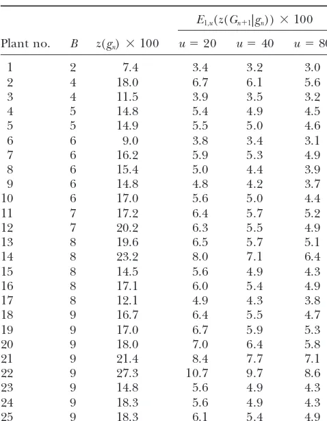
TABLE 3 uted, calculating the proposed selection criteria in addi-tion to the marker scoreBprovides additional information
Selection criteria for the 25 BC1plants with highest marker
to assess the value of backcross individuals and can assist
scoreBin the sample data set for sugar beet
geneticists and breeders in their selection decision.
consisting of 89 plants
QTL introgression:Marker-assisted selection in
intro-E1,u(z(Gn⫹1|gn))⫻100 gression of favorable alleles at quantitative trait loci (QTL) usually comprises selection for (1) presence of the do-Plant no. B z(gn)⫻100 u⫽20 u⫽40 u⫽80
nor allele at two markers delimiting the interval in which 1 2 7.4 3.4 3.2 3.0 the putative QTL was detected and (2) the recurrent 2 4 18.0 6.7 6.1 5.6 parent allele at markers outside the QTL interval. Our 3 4 11.5 3.9 3.5 3.2 results can be applied for the latter purpose in exactly
4 5 14.8 5.4 4.9 4.5
the same way as previously described for the transfer of
5 5 14.9 5.5 5.0 4.6
a single target gene. Hence, our approach is applicable
6 6 9.0 3.8 3.4 3.1
to many scenarios in application of marker-assisted
back-7 6 16.2 5.9 5.3 4.9
crossing for qualitative and quantitative traits.
8 6 15.4 5.0 4.4 3.9
9 6 14.8 4.8 4.2 3.7 We thank Dietrich Borchardt for critical reading and helpful
com-10 6 17.0 5.6 5.0 4.4 ments on the manuscript. We are indebted to KWS Saat AG, 75555
11 7 17.2 6.4 5.7 5.2 Einbeck, Germany, for providing the experimental data on sugar beet.
12 7 20.2 6.3 5.5 4.9 We greatly appreciate the helpful comments and suggestions of an
13 8 19.6 6.5 5.7 5.1 anonymous reviewer.
14 8 23.2 8.0 7.1 6.4
15 8 14.5 5.6 4.9 4.3
16 8 17.1 6.0 5.4 4.9
LITERATURE CITED
17 8 12.1 4.9 4.3 3.8
18 9 16.7 6.4 5.5 4.7 Bartlett, M. S., andJ. B. S. Haldane, 1935 The theory of
inbreed-19 9 17.0 6.7 5.9 5.3 ing with forced heterozygosity. J. Genet.31:327–340.
Bernardo, R., 2002 Breeding for Quantitative Traits in Plants. Stemma
20 9 18.0 7.0 6.4 5.8
Press, Woodbury, MN.
21 9 21.4 8.4 7.7 7.1
David, H. A., 1981 Order Statistics. Wiley, New York.
22 9 27.3 10.7 9.7 8.6
Franklin, I. R., 1977 The distribution of the proportion of genome
23 9 14.8 5.6 4.9 4.3 which is homozygous by descent in inbred individuals. Theor.
24 9 18.3 5.6 4.9 4.3 Popul. Biol.11:60–80.
25 9 18.3 6.1 5.4 4.9 Fisher, R. A., 1949 The Theory of Inbreeding. Oliver & Boyd, Edinburgh.
Frisch, M., M. BohnandA. E. Melchinger, 1999a Minimum
sam-For details and explanation of z(gn) and E1,u(z(Gn⫹1|gn)) ple size and optimal positioning of flanking markers in marker-see text. assisted backcrossing for transfer of a target gene. Crop Sci.39:
967–975 (erratum: Crop Sci.39:1913).
Frisch, M., M. BohnandA. E. Melchinger, 1999b Comparison
of selection strategies for marker-assisted backcrossing of a gene. Crop Sci.39:1295–1301.
1–9 were 90, 102, 78, 84, 102, 89, 75, 94, and 94 cM. Haldane, J. B. S., 1919 The combination of linkage values and the calculation of distance between the loci of linkage factors. J.
After producing the BC1generation, 89 plants carrying
Genet.8:299–309.
the target gene were preselected and analyzed for the
Hanson, W. D., 1959 Early generation analysis of lengths of
hetero-25 markers. The criteriaB,z(gn), andE1,u(z(Gn⫹1|gn)) for zygous chromosome segments around a locus held heterozygous with backcrossing or selfing. Genetics44:833–837.
u⫽20, 40, and 80 were calculated and presented for the
Hill, W. G., 1976 Order statistics of correlated variables and
implica-25 plants with the smallest marker scoresB(Table 3). tions in genetic selection programmes. Biometrics32:889–902. We refer here only to the most interesting results: Hill, W. G., 1993 Variation in genetic composition in backcrossing
programs. J. Hered.84:212–213.
1. Plant 6 hadz(gn)⫽ 9.0% and plant 10 hadz(gn)⫽ Hillel, J., T. Schaap, A. Haberfeld, A. J. Jeffreys, Y. Plotzky
et al., 1990 DNA fingerprints applied to gene introgression in
17.0%, in spite of an identical marker score ofB⫽6.
breeding programs. Genetics124:783–789.
2. Plant 1 was the best with respect to all three criteria. Hospital, F., andA. Charcosset, 1997 Marker-assisted introgres-However, plant 6 was second best with respect to the sion of quantitative trait loci. Genetics147:1469–1485.
Hospital, F., C. ChevaletandP. Mulsant, 1992 Using markers in
expected donor genome proportion but had only
gene introgression breeding programs. Genetics132:1199–1210.
rank 6 with respect to the marker scoreB. Markel, P., P. Shu, C. Ebeling, G. A. Carlson, D. L. Nagleet al., 3. Plant 9 had a considerably larger expected donor ge- 1997 Theoretical and empirical issues for marker-assisted
breed-ing of congenic mouse strains. Nat. Genet.17:280–284.
nome proportion [z(gn)⫽14.8%] than plant 17 [z(gn)⫽
Maurer, H. P., A. E. MelchingerandM. Frisch, 2004 Plabsoft:
12.1%], but the expected donor genome proportion software for simulation and data analysis in plant breeding. Pro-in the best progeny of plant 9 was lower than that ceedings of the 17th EUCARPIA General Congress, September
8–11, 2004, Tulln, Austria, pp. 359–362.
of plant 17 for all three populations sizes.
Ribaut, J.-M., C. JiangandD. Hoisington, 2002 Simulation
experi-ments on efficiencies of gene introgression by backcrossing. Crop
These results demonstrate that the criteriaB,z(gn), and
Sci.42:557–565.
E1,u(z(Gn⫹1|gn)) can result in different rankings of indi- Stam, P., 2003 Marker-assisted introgression: Speed at any cost?,
pp. 117–124 inEUCARPIA Leafy Vegetables 2003, edited byTh. J. L.
distrib-Valencia, Spain. J. Hered.87:136–138.
Stam, P., andA. C. Zeven, 1981 The theoretical proportion of the Visscher, P. M, 1999 Speed congenics: accelerated genome
recov-donor genome in near-isogenic lines of self-fertilizers bred by ery using genetic markers. Genet. Res.74:81–85. backcrossing. Euphytica30:227–238.
Visscher, P. M, 1996 Proportion of the variation in genetic composi- Communicating editor: R. W.Doerge
APPENDIX A
We use here an abbreviated notation:Gi,j(i⫽1 . . .c,j⫽1 . . .mi) is a random variable taking 1 if thejth marker on theith chromosome is heterozygous and 0 otherwise.
We derive the variance ofBin a BCn population under the assumptions of (1) no selection in generations BCs (s⬍ n) and (2) no preselection for presence of target genes in generation BCn(i.e., the entire BCnpopulation is considered, comprising individuals carrying the target genes as well as individuals not carrying the target gene). We have
var(B)⫽ var
冢
兺
1ⱕiⱕc1ⱕ
兺
jⱕmiGi,j
冣
⫽兺
1ⱕiⱕc1ⱕ兺
jⱕmivar(Gi,j) ⫹ 2
兺
1ⱕiⱕc1ⱕ
兺
jⱕmij⬍兺
j⬘ⱕmicov(Gi,j,Gi,j⬘).
Under assumptions (1) and (2) we have for anyGn,i,j
var(Gi,j)⫽ 1 4
1 2n
冢
1⫺1 2n
冣
⫽1 2n⫹2⫺
1 22n⫹2
(Hill1993) and further
cov(Gi,j,Gn,i,j⬘)⫽ 1 4
1
2n
冢
(1⫺ri,j,j⬘) t⫺ 12n
冣
⫽(1⫺ri,j,j⬘)n 2n⫹2 ⫺
1 22n⫹2
(Visscher1996) with
ri,j,j⬘⫽r(xi,j⬘⫺ xi,j).
Therefore,
var(B)⫽m
冢
12n⫹2⫺
1
22n⫹2
冣
⫹ 2冢
⫺k22n⫹2⫹
1 2n⫹2
兺
1ⱕiⱕc1ⱕ
兺
jⱕmij⬍兺
j⬘ⱕmi(1⫺ ri,j,j⬘)
冣
,where
k⫽
兺
1ⱕiⱕc(mi⫺ 1)2/2
is the number of covariance terms.
We derive cov(B,Z) under assumptions (1) and (2). Because
E(BZ)⫽ E
冢冤
兺
1ⱕiⱕc1ⱕjⱕm兺
iGi,j
冥冤
兺
1ⱕi⬘ⱕcyi⬘
yZi⬘
冥冣
⫽ E冢
1ⱕiⱕc兺
1ⱕjⱕm兺
i兺
1ⱕi⬘ⱕc Gi,j
yi⬘
yZi⬘
冣
⫽1ⱕiⱕc兺
1ⱕjⱕm兺
i
兺
1ⱕi⬘ⱕc E
冢
Gi,jyi⬘
yZi⬘
冣
and
E(B)E(Z)⫽E
冢
兺
1ⱕiⱕc1ⱕ兺
jⱕmiGi,j
冣
E冢
兺
1ⱕi⬘ⱕcyi⬘
yZi⬘
冣
⫽冤
1ⱕ兺
iⱕc1ⱕ兺
jⱕmiE(Gi,j)
冥冤
兺
1ⱕi⬘ⱕcE
冢
yi⬘ yZi⬘冣冥
⫽
兺
1ⱕiⱕc1ⱕjⱕm
兺
i兺
1ⱕi⬘ⱕc
E(Gi,j)E
冢
yi⬘
yZi⬘
冣
we have
cov(B,Z)⫽ E(BZ)⫺E(B)E(Z)⫽
兺
1ⱕiⱕc1ⱕ
兺
jⱕmi1ⱕ兺
i⬘ⱕcyi⬘
ycov(Gi,jZi⬘)
and from
cov(Gi,jZi⬘)⫽0 fori⬆ i⬘ follows
cov(B,Z)⫽
兺
1ⱕiⱕc1ⱕ
兺
jⱕmiyi