ABSTRACT
BHARATHI, AKILAN. Optimal Feed-Rate Scheduling and Trajectory Control for Micro/Nano Positioning Systems. (Under the direction of Dr. Jingyan Dong.)
This thesis focuses on an approach for exploiting the dynamic capabilities of a Micro/Nano positioning system for optimal Feed-Rate scheduling to trace a given trajectory in optimal time. To achieve minimal time contouring, the capabilities of the system are exploited and identified fully than just concentrating on the controller and the control algorithms.
Enormous effort has been spent by the research community on advanced feedback control algorithms and techniques in comparison to improving the system performance through detailed trajectory planning and feed-rate scheduling. In high-rate contouring, significant accuracy can be realized through consideration of dynamic system capabilities and trajectory planning with respect to constant velocity profiles of the actuator. In the present work, the dynamic system capabilities of a piezoelectric actuator and a nano-positioning stage are identified and employed within a feed-rate scheduling algorithm. The intended result is a time-optimal (minimum time) trajectory that fully utilizes the dynamic capabilities of the system, since one important concern in high-speed contouring is when the command input exceeds the physical capabilities of the system and the resulting errors. The errors caused by this source cannot be addressed solely through improvements in controllers. Trajectory planning is required to ensure that infeasible commands are never requested of the individual axes on the positioning stage.
incorporation of these models in the feed-rate optimization algorithm. We used a flexure based high-bandwidth nano-positioning stage actuated by piezoelectric actuators as the testbed for the purpose of identification of the dynamic capabilities of the system. In this work the actuator limitations are taken into consideration where the feasible velocities and accelerations of a particular axis are constrained with respect to the displacement from its initial position. The other constraints of the nano-positioning stage come from the frequency components of command signals, which contain frequency components in excess of the system capabilities. The bandwidth limitations are introduced to mitigate such frequency related problems encountered when traversing sharp geometric features at high velocities. The work also presents an approach to trajectory planning and a computationally efficient algorithm for generating a minimum-time feed-rate profile subject to the above constraints.
Finally the detailed simulation results demonstrate the improvements in trajectory tracking through the use of such a model-based feed-rate optimization approach. The results are compared with common industry practices where the system traces the given trajectory at constant feed-rate. The algorithm is tested on various complex trajectories with sharp corners and rapid turns that include hermite curves (cubic spline trajectories) and zigzag scanning linear trajectories that is widely used in Atomic Force Microscopes. The results demonstrate the effectiveness of using the approach of trajectory planning and feed-rate scheduling in comparison to the approach of developments and fine-tuning of controllers only. An
Optimal Feed-Rate Scheduling and Trajectory Control for Micro/Nano Positioning Systems
by Akilan Bharathi
A thesis submitted to the Graduate Faculty of North Carolina State University
in partial fulfillment of the requirements for the Degree of
Master of Science
Industrial Engineering
Raleigh, North Carolina 2013
APPROVED BY:
_________________________ ___________________________
Dr. Yuan-Shin Lee Dr. Chih-Hao Chang
___________________________ Dr. Jingyan Dong
DEDICATION
I sincerely dedicate this work to my mother Dr. Rajeswari Bharathi, my father Mr. Bharathi
Govindswamy and my mentor Mr. R. Kesavachar. I am very grateful to god for all his blessings and faithfully dedicate this work to him as well. Finally, I would also like to dedicate this work to my brother Mr. Aadhithan Bharathi who has been very supportive in my life.
BIOGRAPHY
Akilan Bharathi was born in Madurai, Tamil Nadu, India on June 18th, 1990. He obtained his bachelor’s degree in Electronics and Instrumentation Engineering from Hindustan College of
Engineering affiliated Anna University, Chennai, Tamil Nadu, India in 2011. After
ACKNOWLEDGEMENTS
I would first like to thank and acknowledge this work to Dr. Jingyan Dong, my academic advisor, for his guidance and help, which was significant in the completion of this work. I would also to thank all my professors and other faculty and staff who have been a part of my graduate career. I also thank the laboratory personnel and Ph.D. scholars for their help, advice and support.
Thanks to my dear mother Dr. Rajeswari Bharathi, my respected father Mr. Bharathi
Govindswamy, and my esteemed mentor Mr. R. Kesavachar for their support, motivation and encouragement without which I would not have got an opportunity to be a part of the
wolfpack and my master’s experience would have been difficult to fulfill. I also want to
TABLE OF CONTENTS
LIST OF TABLES ... vi
LIST OF FIGURES ... vii
CHAPTER 1: INTRODUCTION ... 1
CHAPTER 2: MODELING AND IDENTIFICATION OF A NANOPOSITIONING SYSTEM ... 9
2.1 Introduction ... 9
2.2 Constraints Arising from Actuator Limitations ... 10
2.3 Displacement Dependency of Actuator constraints. ... 15
2.4 Parallel Kinematic XY Stage ... 26
2.5 Identification of Feasible Region ... 33
2.6 Frequency Constraints arising from Curved Trajectories ... 38
2.7 Conclusion ... 40
CHAPTER 3: MINIMUM-TIME FEED-RATE OPTIMIZATION ... 41
3.1 Introduction ... 41
3.2 Trajectory Planning ... 43
3.3 Feed-Rate Scheduling ... 49
3.4 Conclusion ... 57
4.1 Simulation Model and Parameters ... 59
4.2 Comparative Trajectory ... 61
4.3 Test Results for Linear Trajectory ... 62
4.4 Test Results for Cubic Spline Trajectory ... 68
4.5 Discussions ... 80
CHAPTER 5: CONCLUSION AND FUTURE WORK ... 82
LIST OF TABLES
Table 1: Controller Parameters ... 30
Table 2: Performance Parameters ... 30
LIST OF FIGURES
Figure 1: Parallelogram Constraints on an Axis ... 13
Figure 2: Feasible Region at Initial Position... 17
Figure 3: Feasible Region at Maximum Displacement... 19
Figure 4: Feasible Performance Envelope ... 21
Figure 5: Experimental Response to Open-Loop Command Reversals for 20% Magnitude . 23 Figure 6: Experimental Response to Open-Loop Command Reversals for 2% Magnitude ... 24
Figure 7: Parallel Kinematic XY Stage ... 27
Figure 8: Frequency Response of a single axis of the XY Stage ... 28
Figure 9: Closed Loop Step Response of a single axis of the XY Stage ... 29
Figure 10: Closed Loop Step Response of a single axis of the XY Stage ... 31
Figure 11: Effects of Overshoot using a Controller with overshoot ... 32
Figure 12 Effects of Oscillatory Response using a Controller with overshoot ... 33
Figure 13 Mismatch of Feasible Region Identification ... 34
Figure 15: Delay in obtaining maximum Acceleration ... 36
Figure 16: Comparison in Number of Intervals in Parametric Variable ... 44
Figure 17: Estimation of Path Curvature ... 47
Figure 18: Simulation Model for a Single Axis of the Positioning Stage ... 60
Figure 19: Desired Trajectory and its Planning ... 62
Figure 20: Velocity, Acceleration and Parametric Velocity Profile ... 63
Figure 21: Results of Scheduling within Feasible Envelope for X-axis ... 64
Figure 22: Results of Scheduling within Feasible Envelope for Y-axis ... 65
Figure 23: Results for Constant Velocity... 66
Figure 24: Results for Optimal Algorithm ... 66
Figure 25: Performance at Right-side Corners ... 67
Figure 26: Performance at Left-side Corners ... 67
Figure 27: Trajectory Planning of a Cubic Spline Trajectory ... 69
Figure 28: Velocity, Acceleration and Parametric Velocity Profiles ... 70
Figure 30: Results of Scheduling within Feasible Envelope for Y-axis ... 72
Figure 31: Results for Optimal Algorithm ... 73
Figure 32: Results for Constant Velocity... 73
Figure 33: Tracking performance at curve... 74
Figure 34: Velocity, Acceleration and Parametric Velocity Profile after inclusion of Frequency Constraint ... 75
Figure 35: Results of Scheduling within Feasible Envelope for X-axis ... 77
Figure 36: Results of Scheduling within Feasible Envelope for Y-axis ... 77
Figure 37: Results for following Optimal Algorithm commands ... 78
Figure 38: Results for tracing at constant speed in same time ... 78
CHAPTER 1: INTRODUCTION
Micro/nanotechnology has become increasingly important for the economy and the industry over the recent years. Broadly, the term nanotechnology means “the study, development and
processing of materials, devices and systems in which structure on a dimension of less than
100nm is essential to obtain the required functional performance” [1]. As a reference, the
features seeable by unaided human eye are in the order of around 10 um. Micro/Nano
technology is gearing up faster due to the demands of compact products, high bandwidth and high sensitivity. Miniaturization, though expensive, rewards us with better integrity, energy and material efficiency, and unrevealed opportunities for new devices and new applications.
Currently, Micro/Nano technology has been increasingly applied to many industries from aerospace and automotive industry to telecom industry to medical and biomedical industry. For example, it is used in the instrumentation industry to fabricate atomic force microscope (AFM) tips which require nanometer accuracy. In addition, micro-scale features in sensors, and actuators are common in electronic industry. With such rapid developments and
increasing applications of micro/nano technology, “The improvements in machinery for manufacturing of microstructures must keep pace with the developments with the micro/nano
technology.” [2].
nano-positioners have been used to scratch metal surface at nanometer scale [4]. Other than just precision and accuracy, in industry, the cycle time and production time are also an important measure of the manufacturing performance. The minimum-time control and feed-rate
scheduling algorithms satisfy both, the requirements for precision and throughput of manufacturing.
Significant effort has been spent in the research community to improve the contouring and scanning performance of high-speed nanopositioning systems. Majority of these efforts has focused on advances in low level feedback control techniques. The motion control structure can be divided into 2 levels where the tracking control is considered to be lower level and the trajectory planning as the upper level [6]. Trajectory planning is very important as it is the results of the path planner that provides reference points for the path tracker. The path tracker is normally a linear feedback controller like a PID controller which tries to minimize the deviation of the actual position from the desired reference position. However, the
dynamic system. The subject of the present work is to provide a framework for abstracting the capabilities of an individual multiaxis nano-positioning system and a methodology for using these capabilities to generate a time-optimal feed-rate profile for a particular pre-known trajectory on a particular system.
Given a multi-axis trajectory, the velocity and acceleration of a particular multi-axis positioning system is necessarily constrained by the limitations of the actuator. The identification of a feed-rate profile such that the actuator is not requested of velocities or accelerations beyond its capabilities at any point on the trajectory is a non-trivial
optimization problem and has received significant attention from the research community in robotics and manufacturing literature as well.
Several Researchers have addressed the time-optimal control problem. Lynch, P. M. [18] developed a specialized minimum-time algorithm assuming constant bounds for the actuators. Bobrow, Dubowsky and Gibson [5] came up with a solution to find acceleration profiles such that at each acceleration point, the actuator delivers the maximum velocity possible which is no greater than the maximum velocity the actuator can provide. The algorithm to find the solution for such acceleration profiles was derived by Bobrow [19] and presented in a minimum-time control problem with specified path constraints and state-dependent actuator constraints [20].
initially divided the problem into trajectory planning and trajectory tracking. This division came with the inability to fully utilize the system’s dynamic capabilities especially with
respect to the trajectory planner. To alleviate this problem and improve the efficiency, Shin and McKay [6] came up with the solution to minimum-time control problem subject to geometric constraints and actuator constraints. The solution was obtained from a trajectory planning algorithm taking into account the details of the dynamics of the robotic manipulator. Bobrow, Dubowsky and Gibson [5] tried standard optimal control methods for the solution and they recorded that the numerical algorithms were computationally rigorous. In general they all came up with an algorithmic to achieve the solution of minimum-time control problem for robotic actuators. They proved the importance and advantages of trajectory planning which made trajectory tracking a simpler task than it was earlier.
Several others, later, followed this concept and idea of references [5] and [6]. The application of their methods in practice was done by Dahl [7] and [22]. They addressed the case where there might be disturbances and modeling errors when the torque, delivered by the actuators of a robotic manipulator, is at its limit. In such cases where the torque/force margin of the actuator gets saturated to its maximum possible limit and there are still deviations in tracking the specified path due to disturbances and modeling errors, he proposed the solution with the implementation of a path velocity controller in addition to the preprocessed optimal velocity scheduling algorithm. This path velocity controller acts as a feedback controller outside the ordinary robot controller and it modifies the nominal velocity profile computed by the
wiser utilization of the available torque range. He also demonstrated the ability of the path velocity controller in compensating for the time-variations in the robot dynamics.
Cao, Dodds and Irwin [8] addressed the problem of smooth constrained path planning and time-optimization in a new approach. They optimize the movement of the robotic joint paths rather than that of the end-effector. An objective function is found that combines the
can be used for optimization purposes to improve many other parameters involved in high-speed contouring rather than just a time-optimum trajectory.
Zlajpah [9] focused on a solution to the optimal trajectory planning problem subject to joint torque constraints, joint velocity constraints and task constraints. He follows the approach of Bobrow [5] and Shin and McKay [6] in developing an algorithm that takes into account other constrainable factors in addition to the torque bounds of references [5] and [6]. He also accounted for the detailed model of the manipulator dynamics in calculating the optimized trajectories.
Several other authors studied the minimum-time control problem like Kahn and Roth [25] assumed constant torque limitations and non-constrained path and different aspects of the problem are presented in [23], [24], [26] and [27].
Butler and Tomizuka [10] approach the problem analytically for machine tools. The operating space of admissible motion formed by the torque versus velocity is overly constrained and the solution of a differential equation gives a uniquely defined trajectory. The difference is that they do not arrive at the trajectory through the solution to an
optimization problem.[17]. Farouki, Tsai and Wilson [11] studied the problem and
Imamura and Kaufman [12], [13] decompose the federate optimization problem into two phases. The first phase is to identify a minimal tracking time through nonlinear programming techniques with respect to feed rate profile subject to contour error constraints and the second phase is to tune a controller subject to the actuator power constraints. However, it is unlikely that the nonlinear programming algorithm will always identify a globally optimal federate profile due to the non-convex character of the feasible space. The idea of varying controller gains for optimal control is interesting; but with respect to practical implementation in commercial machines, this apporach raises concerns and hence might not gain acceptance since the controllers in the market typically do not permit changes to internal controller gains. Also only limited simulation results are presented for a simple contour.
In the manufacturing literature, Renton and Elbestawi [14] have come up with a
computationally efficient two-pass algorithm to solve the feed rate optimization and planning problem to obtain a minimum-time feed-rate profile. The algorithm scans the trajectory twice; once in the forward direction and once in the reverse direction. In the first scan, also called as forward pass, the largest possible parametric acceleration is assigned to all the parametric segments in the trajectory subject to the performance envelope constraints. In the second scan, also called as the backward pass, the same procedure is repeated with the same constraints and an additional constraint that the parametric velocity now assigned should be lesser than or equal to that assigned in the forward pass. Bieterman and Sandstorm [15] have published a structurally similar two-pass feed-rate optimization algorithm developed
Dong and Stori [17] developed a feed-rate optimization algorithm modeled similar to the framework of Renton and Elbestawi [14] taking into account the dynamic system
capabilities. They have also come up with a detailed model that addresses the contour error and have incorporated the contouring accuracy into the algorithm.
CHAPTER 2: MODELING AND IDENTIFICATION OF A NANOPOSITIONING SYSTEM
2.1 Introduction
Positioning with resolution in the order of nanometer is very important for many modern technologies, especially in domain of micro/nano technology. Micro/Nano positioning systems are widely used in various applications, such as ultrafine focusing of optical assemblies and optical alignment [28], [29], scanning probe microscopes such as STM, AFM, MTA, SNOM, etc… [30], [31] and micro/nano manufacturing [32], [33], [34] and
[35]. Piezoelectric stack actuators and high resolution displacement actuators are widely used to obtain displacement with nanometer resolution. There are many other actuators that can be used for micro and nano positioners that work with almost all actuation principles like
“inchworm” actuators, electromechanical actuators, etc… [36] Each axis of the
micropositioner or nanopositioner is actuated individually by each of these actuators. A linear amplifier is connected to each of these actuators to have a linear steady-state
identify this feasible region so that the controller does not request velocities and accelerations beyond the actuators capabilities.
Initially, the limits on the actuator velocity and actuator acceleration were assumed to be constant [26] and [27]. Later the assumption was improved by considering the bounds on actuator velocity and actuator acceleration to be piecewise constant [16] and [17]. This is still dangerous because the piecewise assumptions makes it overly conservative or opens up the probability for controller to command infeasible accelerations at a given velocity.
2.2 Constraints Arising from Actuator Limitations
In our case, we use piezoelectric stack actuators to actuate each axis of the positioning stage. They work on the principle of inverse piezoelectricity where an applied electrical field results in internal generation of a mechanical strain. This strain is constructively utilized in micro and nano manipulation of each axis of the positioning stage. Conventionally the force of an actuator is modeled as directly proportional to the voltage supplied. An analogous constant of proportionality exists between voltage and the actuation force of the piezoelectric actuator.
(1)
an ideal second order model should be sufficient to capture majority of the low frequency dynamic behavior of a single axis of the positioning system.
̈ ̇ (2)
Where ‘x’ in the above equation represents the displacement of an individual axis, ̇ represents the velocity and ̈ represents the acceleration of a single axis of the positioning system. The force delivered by a single axis is represented by ‘F’ and the variables ‘M’, ‘b’ and ‘k’ represent the mass, damping co-efficient and spring constant/stiffness respectively of
a single axis of the positioning system. The above equation can be generalized in terms of constants as shown below.
̈ ̇ (3)
Where, , and represent the inertial, viscous frictional and elasticity characteristics respectively of the design, structure and configuration of the single axis of the positioning system.
In the case of an actuator, the maximum actuator force will be the primary system limitation. From equation (3), we see that the linear combination of the displacement, velocity and acceleration must be constrained at all times within the maximum and minimum limits of the actuator force. This helps in defining the bounds for velocity and acceleration and identifying the performance envelope i.e. the feasible values of velocity and the feasible values of
̈ ̇ (4)
Where, represents the magnitude of maximum force output by an actuator in positive direction and similarly represents the magnitude of maximum force exhibited in
negative direction. Since we have the trajectory before in hand, it provides us with the actual displacement position during the trajectory planning stage making displacement a known quantity rather than an unknown variable. The bounds for the actuator constraints now include the displacement term leaving the velocity and acceleration of the actuator constrained. The constrained actuator equation now becomes,
̈ ̇ (5)
Under the assumption of such an ideal second order dynamic system with a fixed actuator output and constant inertial and viscous friction coefficients, the maximum feed rate is achieved when all the driving force is used to overcome the viscous friction. At this condition, the velocity given by the actuator is the maximum possible velocity and at this maximum velocity, there will be no acceleration possible in the forward direction. Again at this maximal forward velocity, the reversed acceleration will be maximized. The maximum velocity and the minimum acceleration, in terms of the maximum force output of the actuator are,
At v= (6)
(8)
Similarly, the minimum feed-rate is achieved when all the driving force is spent on the viscous friction. At this minimum velocity there will be no acceleration possible in the reverse direction i.e. deceleration capabilities are zero and the forward acceleration
capabilities will be at its maximum. The minimum velocity and maximum acceleration, in terms of the actuator force output are,
At v=
(9)
(10)
(11)
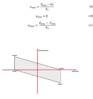
The above constraints result in a feasible parallelogram within the acceleration versus velocity space for a particular axis at a particular displacement as shown in Figure (1).
Similar constraints without the displacement parameter have been introduced previously by authors and showed significant improvement from over the common assumption of a constant maximum acceleration for an axis independent of its velocity. Such a dynamic feasible region also performs better compared to the piecewise constant bounds on
acceleration depending on the velocity of the individual axis as mentioned earlier due to an overly conservative modeling of the feasible region or a feasible region that can still lead to demands of incapable velocity and acceleration outputs by the linear controller [16] and [17]. Such feasible regions of velocity versus acceleration are termed as performance envelopes and Renton and Elbetsawi [14] demonstrate the experimental and higher-order simulated single-axis performance envelopes, in which the dynamic behavior of the actual complex system is approximated reasonably well by such parallelogram performance envelopes. Here in this work we have introduced the displacement ‘x’ as a parameter in developing the
2.3 Displacement Dependency of Actuator constraints.
From, the above expressions for and from equations (6) and (9), we notice that they are dependent on a third dimension: “the displacement.” In all the above references we
have cited, the performance envelope was one single envelope and did not vary with any other variable. In our case, the actuator constraints of a single-axis are now transformed into state-dependent constraints and are arbitrary functions of the displacement of that particular individual axis. It should also be noticed that the difference between maximum and minimum acceleration of either axis is not dependent on the displacement. This makes the breadth of the performance envelope constant. Similarly, though the maximum velocity and minimum velocity of an individual axis are dependent on the magnitude of the displacement of that axis, their difference i.e. the width of the performance envelope is constant as shown in the equation below.
(12)
This demonstrates that the performance envelope is a constant area envelope moving linearly along the third dimension: “displacement.” The actuator constraints are now varying making the performance envelope three-dimensional in nature. By substituting the initial and final values of displacement for the actuator in our application, we get a corresponding three-dimensional feasible region that addresses only that single particular actuator.
they are commanded to give a negative displacement, they might contract each other and might even lead to breakage of the crystals destroying the entire actuator. The actuator is used for displacements in positive direction only and this makes our minimum achievable displacement to zero. Since, there is not going to be any displacement in the negative direction, there is not going to be any force output in the negative direction and this makes the minimum force output by the actuator to be zero. The left bound of out actuator
constraint equation (5) can now be reduced to as follows,
̈ ̇ (13)
Now, initially when the actuator is at rest i.e. the minimum velocity i.e. the maximum reverse velocity is zero and this makes the maximum reverse acceleration i.e. to also be zero since the actuator cannot displace in that direction. The maximum forward acceleration is at its true maximum at and it is the same as equation (11). Now the
maximum forward velocity is determined by the maximum displacement deliverable by the actuator of that corresponding axis. Since the actuator is starting from the rest position, the maximum displacement given by the actuator in the forward direction is represented by
and maximum feed-rate is achieved when all the driving force is used to overcome the viscous friction. From equation (13), considering the forward direction i.e. right bounds only, for the actuator starting from rest, the variables of the performance envelope are given by
(15)
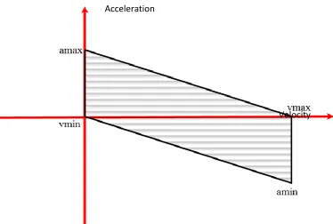
The maximum acceleration and minimum acceleration are the same as that of equations (7) and (8). The velocity-acceleration feasible region for the initial position of the actuator takes the form shown in figure (2) below. As you will notice, there is maximum forward acceleration available at start and the velocity with which the actuator can travel is also at its maximum at this initial zero displacement position.
Figure 2: Feasible Region at Initial Position Acceleration
The below paragraphs and equations will now frame the feasible region at the maximum displacement position as it was done for the home position of the actuator.
As reasoned above, for the final position of the actuator along a particular axis, the entire driving force is spent in reaching the displacement giving rise to the relation
(16)
This gives rise to the conclusion that the maximum forward velocity for the actuator when it is in its maximum displacement position is zero i.e. . The maximum forward acceleration is also zero and the maximum reverse acceleration is same as equation (8). Now, considering the reverse direction of displacement from this maximum displacement position, the maximum driving force of the actuator is represented by is zero and the maximum possible displacement the actuator can get displaced in this direction is . Substituting these values into equation (5) the bounds for the actuator constraints now take the form
̈ ̇ (17)
Now, considering the left bounds of equation (17) i.e. for the reverse direction of motion from the maximum displacement position, we get the variables and the maximum forward and reverse accelerations, i.e. and as follows.
At v=
(20)
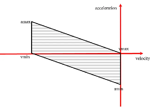
Equations (19) and (20) are same are as equations (10) and (11) respectively. From the above values of variables, the feasible region for the actuator at its maximum displacement
condition looks as shown below in figure (3). You will notice the converse of what was observed in figure (2). Now, the acceleration will be the maximum in the reverse direction and the velocity with which the actuator can travel in the reverse direction is also fully available only at this displacement position.
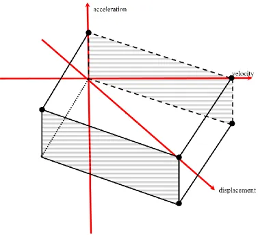
The feasible region for all other values of displacement can be found in a similar fashion and will be a smooth linear transition from the figure (2) to figure (3) where the feasible region would be moving forward along the displacement axis and left along the negative velocity axis as the displacement position keeps increasing. The position, velocity, acceleration and time data were gathered for an individual axis from a parallel kinematic XY stage actuated by a piezoelectric stack actuator using a Delta-Tau PMAC2 motion controller at a sampling rate of 20 KHz. The data verified two results; one was that the values of the
variables , , and had good degree of precision and secondly, they showed the change in their values for different displacement commands. Thus the entire performance envelope for an individual axis actuated by a specific actuator would be like the figure shown below.
Figure 4: Feasible Performance Envelope
The intent of the modeling efforts is to capture the feasible performance envelope of each axis individually so that they can be used in the optimal scheduling of the feed-rate. The most important purpose of the feed-rate scheduling is to understand the maximal forward and reverse accelerations that can be achieved as a function of velocity.
axis to reversing open-loop step commands. Starting the system at rest (zero velocity, zero acceleration and zero displacement) or at a known displacement (and zero velocity and zero acceleration) the following sequence of events is commanded and the system’s response (displacement, velocity and acceleration) is observed.
1. A positive step command signal is given which makes the system accelerate to a maximum forward velocity. The magnitude of the step command decides the magnitude of the displacement.
2. Once the system reaches a steady-state maximum forward velocity (zero forward acceleration), then a negative command signal is given as input. By a negative command signal, it means that now the magnitude of the step input is less than that given in the first step. The system responds by accelerating the maximum possible in the negative
direction. The velocity first approaches zero and then increases in the negative direction. The acceleration will decrease due to the effects of viscous friction and reduced inertia. 3. The system will now reach a steady-state maximum reverse velocity (zero reverse
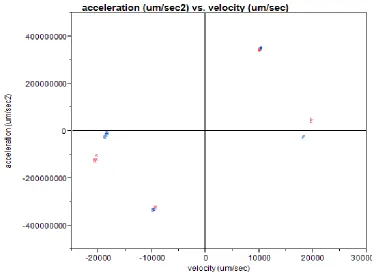
The above sequence of events are repeated for various values of displacement i.e. by giving various reversing magnitudes of step input and recording the corresponding maximum acceleration and velocity values in the forward and reverse directions. This will demonstrate the shifting of the feasible space of velocity versus acceleration. The figures below show two of the experimental responses we got for reversing open-loop commands where the
magnitude in percentage represents the difference in the percentage of the open loop commands. The data shown below were collected per the method explained above.
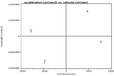
Figure 6: Experimental Response to Open-Loop Command Reversals for 2% Magnitude
open-of the stage, we were not able to get continuous data but were able to get only the extreme maximum points in the negative and positive direction with a single data point in the path to maximum velocity. The data verifies two things, firstly, the parallelogram behavior where the velocity first approaches zero and increases in the other direction and the acceleration always decreases in the other direction. Secondly, the maximum and minimum velocities and acceleration scale almost linearly with the displacement. For a displacement of 0.13 um from the figure 6, the maximum velocity in the forward direction is approximately 1500 um/sec; and from the figure 5 i.e. for a step input that is 10 times in magnitude of step input given for figure 6, the displacement is scaled approximately by 13 times i.e. 1.7 um and the maximum forward velocity is scaled by approximately 12.13 times i.e. 18,200 um/sec. Similarly, from the experimental results, for a step input that is 15 times in magnitude compared to the step input of figure 6, the maximum forward velocity is scaled by approximately 16.67 times i.e. 25,000 um/sec. Hence the maximum forward velocity for all the points of displacement can be scaled from the experimental data we have. This way we can get the maximum forward velocity and maximum reverse velocity for all points of displacement. These values can be used as constraints in the feed-rate scheduling algorithm.
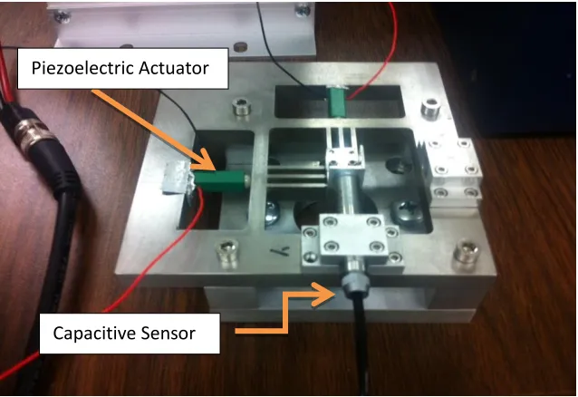
2.4 Parallel Kinematic XY Stage
In micro/nano positioning applications, the system i.e. final positioning element is of major importance. The actuator and the behavior of the positioning of the stage to the actuator commands that has to be studied to frame a proper optimal algorithm to schedule feed-rate.
Figure 7: Parallel Kinematic XY Stage
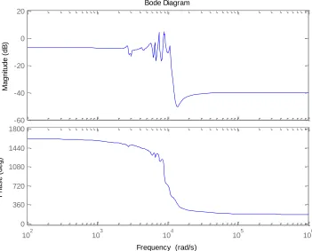
A mathematical model for a single axis of the XY stage was built by getting frequency response data from both the axis individually. The magnitude data and the frequency data were manipulated using the tools of MATLAB simulation software to get a continuous-time higher-order mathematical equation for an individual axis that closely modeled the real-time behavior of a single axis of the stage. Below figure (8) shows the frequency response of an individual axis of the XY positioning stage.
Piezoelectric Actuator
Figure 8: Frequency Response of a single axis of the XY Stage
The frequency constraint developed below is for a single axis of this XY positioning stage. The bandwidth of the individual axis was found from its frequency response shown in the figure (8) above. A continuous-time critically damped PI (Proportional + Integral) controller was then developed and tuned for a unit step input given to each individual axis of the XY stage and the performance parameters and the controller parameters for a controller of the
form are shown below in figure 9. and represent the proportional gain
-60 -40 -20 0 20 M a g n itu d e ( d B )
102 103 104 105 106
0 360 720 1080 1440 1800 P h a s e ( d e g ) Bode Diagram
improving the speed of response and also prevent overshoots; the below values gave the best possible results and maintained the closed-loop stability of the system.
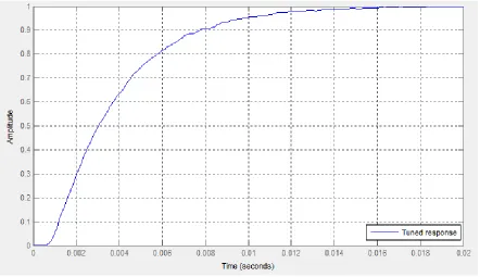
Figure 9: Closed Loop Step Response of a single axis of the XY Stage
Table 1: Controller Parameters
Parameter Symbol Tuned Value
Proportional Gain 0.00022493
Integral Gain 2547391.9453
Table 2: Performance Parameters
Parameter Symbol Tuned Value
Rise Time (seconds) 0.00656
Settling Time (seconds) 0.0127
Overshoot 0 %
Peak 1.00
It might have surprised as to why we are not employing a faster controller in a time
Figure 10: Closed Loop Step Response of a single axis of the XY Stage
Table 3: Performance Parameters for a Faster Controller
Parameter Symbol Tuned Value
Rise Time (seconds) 0.00101
Settling Time (seconds) 0.0131
Overshoot 6.8%
Peak 1.07
The main reason to have avoided this controller than the critically damped controller is the “overshoot.” Though the system was still stable, it gave unsettled oscillations. Even small
oscillations can make high precision tracking unacceptable; the results for using this faster controller is shown below in figures (11) and (12).
Figure 11: Effects of Overshoot using a Controller with overshoot
In the figures (11) and (12) shown above and below, the blue line represents a curved portion of the desired trajectory and the red ‘x’ markers represent how the system has responded to
the desired trajectory. The x-axis and y-axis of the figures represent the ‘x’ and ‘y’ position of the 2-dimensional trajectory respectively. This oscillatory response was noticed in tracing
9.4 9.6 9.8 10 10.2 10.4 10.6 10.8 9.2
9.4 9.6 9.8 10 10.2 10.4 10.6
Results for Optimal Algorithm Traced
Actual
X (um)
Y
(u
m
of linear trajectories as well which made the faster configuration of the controller a highly undesirable one. For high performance contouring, such oscillations or overshoot will
produce adverse results which will spoil the effects of feed-rate scheduling and optimization.
Figure 12 Effects of Oscillatory Response using a Controller with overshoot
2.5 Identification of Feasible Region
The efforts to identify the velocity and acceleration capabilities in the above section were for an open loop system. But now after the implementation of a closed-loop linear feedback controller, the system capabilities have become more limited and it is necessary to verify if
9.96 9.97 9.98 9.99 10 10.01 10.02 10.03 10.04 10.05 9.85
9.9 9.95 10 10.05
Results for Optimal Algorithm Traced
Actual
X (um)
Y
(u
m
this new system still has the same capabilities as the open-loop system. Factors such as the sluggishness to respond for a command input, exhibited by the critically damped controller, are responsible for the change in closed-loop system capabilities. The intuitive reason for the identification of feasible region for the closed-loop system is, the algorithm schedules the feed-rate according to the actual feasible region limits and if that trajectory was commanded to the system where the controller slows the response then the desired trajectory will be heavily short of what is required. The figure (13) shown below pictures the intuitive reply explained before.
Figure 13 Mismatch of Feasible Region Identification
1 2 3 4 5 6 7 8 9 10 11
1 2 3 4 5 6 7 8 9 10 11
Results for Optimal Algorithm Traced
Actual
X axis (um)
Y a
As mentioned above, the blue line and red markers represent the actual trajectory and traced trajectory respectively. Also the x-axis and y-axis represent the ‘x’ and ‘y’ position of the two-dimensional trajectory respectively.
Another important factor that might bother in using the originally identified velocity and acceleration limits are the capability of the closed loop system. The controller should be capable of outputting enough magnitude of the signal to drive the axis at its capable velocity or acceleration. When tried in a simulation environment, the maximum velocity and
acceleration identified for a 1 um step input are shown in the below figure (14) from the gathered data. The data was gathered at a frequency of 1MHz and was plotted to get the velocity graph as the figure (14) shown below.
Figure 14: Velocity Capabilities of the closed-loop system
0 0.01 0.02 0.03 0.04 0.05
Similar set of operations were carried out to identify the maximum acceleration capabilities of the closed-loop system. The data proved the difference in the closed-loop and open-loop capabilities of the system. The open-loop system showed the maximum velocity obtainable as 38,000 um/sec approximately and maximum acceleration as 1.3e+009 um/sec2
approximately when displaced from the initial position 0 um to maximum displacement 15 um. In contrast, the maximum velocity obtained from the closed-loop system as shown in figure (14) for a step input of 1 um is 275 um/sec approximately and the maximum
acceleration delivered is approximately 6e+005 um/sec2. The closed-loop system, hence, has a velocity capability more than 100 times less than the open-loop capability and the
acceleration capability also have reduced by approximately more than 1000 times. The reason for choosing a smaller perturbation is because of the jerk limitations of the system. The below paragraphs show the effects of jerk for a continuous ramp input.
P
o
si
tio
n
(um
)
In the graph shown above, the pink color represents the desired linear trajectory requested of one of the axis and the yellow color represents the response of that axis. Investigating further on the cause for unsatisfactory tracing, we found that the system has slow acceleration capabilities i.e. the system takes significant amount of time to achieve its maximum
acceleration limit. A constant velocity input was feed to the simulation model and the delay in reaching the maximum acceleration can be seen through the figure shown above. From the figure above, it conveys that the system takes time to catch up with the ramp input and once it has caught up with the input, it continues following it with the same slope, i.e. same velocity, as that of the input. The reason to this delay is the jerk exhibited by the system. So if a step input of larger magnitude was used for closed-loop feasible region identification, it would give more time for the acceleration to reach its maximum. Hence the acceleration obtained will not be an instantaneous value. Using such acceleration and velocity values will still produce unsatisfactory tracing results like the one shown in figure (13). Thus we settled for an input of smaller magnitude of excitation like 1 um, where the jerk will be less and the maximum acceleration obtained will be almost instantaneous.
2.6 Frequency Constraints arising from Curved Trajectories
The feasible velocity and acceleration points are found and the feed-rate scheduling algorithm is used to implement these acceleration and velocities with a conventional linear feedback control system. While the actuator velocity and acceleration constraint produce shorter travelling times than conventional techniques, it does not track the given trajectory satisfactorily; other constraints have to be mentioned and specified. A stand-alone feed-back controller will not be able to forcefully track the trajectory. One such important limitation of dynamic systems that will solve this issue is the “Frequency Constraint.”
Although control engineers are very much aware of the closed-loop bandwidth of the entire system during design and tuning of control loops, there is no assurance that the future commands, in the form of geometrically complex high-speed trajectories, will not contain frequency components in excess of the system capabilities. Since we plan the trajectory and schedule a corresponding feed-rate, the path geometry is known before in hand and makes it possible to constrain the command signals so that it is always below the known constraints of the frequency tracking abilities of the individual axes.
Srinivasan and Kulkarni [37], Chuang and Liu [38] and Yeh and Hsu [39] have published variations of tangential approximation approach to the path geometry. Koren and Lo [40] and Takahashi and Bickel [41] use a curvature circle approximation to account for contour errors in their articles. We also rely on an estimate of the instantaneous path curvature ‘k’ and the velocity identified by the feed-rate scheduling algorithm v(t), to calculate the dominant frequency that will be experienced by each of the individual axis. The dominant frequency of magnitude ω is then found from the equation below,
(21)
If an appropriate limiting bandwidth is identified for each of the axes, then the above expression will act as a constraint in identifying the optimal tangential path velocity. This constraint will be vital in traversing sharp curves and turns and is a function of the path curvature.
It is important to note that this limiting bandwidth ω of each individual axis will be
significantly lower than the bandwidth of the entire system including the feedback control loop. The frequency content of the command signal following the above constraint will be considerably lower than the frequency of signals generated by the controller whose limiting bandwidth is given by . The bandwidth for a control loop having a transfer function G(s) is the frequency from zero to the point where the magnitude of the transfer function becomes 0.707|G(0)|. This conventional definition of bandwidth is not suitable for ensuring
2.7 Conclusion
CHAPTER 3: MINIMUM-TIME FEED-RATE OPTIMIZATION
3.1 Introduction
For most of the practical contouring and robotic applications in the world and industry, the trajectory to be followed is known before in hand. It would be a wise practice to make use of this known information than to rely on linear feedback controllers that try to control the trajectory tracking instantaneously. This chapter walks through the phases of planning a trajectory and scheduling an optimal continuous feed-rate profile throughout the trajectory.
Richard Bertsche, of Bertsche Engineering, a manufacturer of high speed machine tools throws light on the importance of acceleration in high speed machining process [44]. He notes that for two different machines with similar velocity capabilities but different
acceleration capabilities, the total processing time might differ by up to 50% when cutting a moderately sized pocket. In practical machining tasks, a high speed machine tool spends most of its time accelerating and decelerating [45]. Fatigue and degradation of the
performance of the actuator is unnecessarily hastened by the extreme acceleration demands placed on the actuators. In such cases, proper demands of accelerations for corresponding velocities can have tremendous impact on both the production time and contouring performance.
Even with the latest advances and improvements in the feedback control, we are not able to address the concerns of optimum-time i.e. how fast the system can trace the trajectory
is not the right solution for such a problem because, they will consume more energy, space and for applications like robotics where such actuators are hosted on the moving platforms, such big sized actuators become concerns of dynamics of the moving platforms making the system heavily non-linear. Butler and Tomizuka [10] pointed out that there is very little attention paid to the subject of trajectory generation for linear systems. Their statement still holds true. The solution to the above problem is through the methods of trajectory
planning/trajectory generation and feed-rate scheduling. Such methods try to utilize the entire dynamic capabilities of the complex systems getting efficient returns out of it. These methods make no compromise on the control/accuracy requirements and still satisfy the industry’s needs such as shorter cycle time, increased life of machine tools and actuators, minimum energy consumption and so on.
Such high-speed trajectory tracking concerns have started bothering the domain of micro-/nanomachining. With advancements in equipment for micro/nanotechnology and demands of consumers for smaller and efficient systems, the trajectory planning and feed-rate
scheduling approach has to be extended to micro-/nano-manufacturing. There are many serial processes such as printing of photolithography masks by electron-beam microscopes, etc… and many serial visualization devices such as AFM, Scanning Electron Microscopes etc…
which loudly call for faster tracking capabilities.
work of Dong, J. and Stori J.A. [17] using the constraints developed in chapter 2 for micro/nano manipulation applications. The below subchapters give a detailed method and approach to trajectory planning and achieving optimal feed-rate scheduling.
3.2 Trajectory Planning
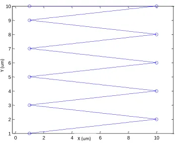
Any given trajectory will have important coordinate points that have the potential to define the trajectory. The trajectory is then reconstructed from these points through mathematical interpolation techniques. A few examples of such interpolation techniques are the hermite interpolation which will form a cubic curve between two given points; similarly linear interpolation will join two specified points by a perfect straight line; and so on there are many other similar interpolation techniques. This interpolation is then considered the trajectory to be followed by our machine tool. If we want a higher degree of precision to a given trajectory, we can just increase the number of points that define the trajectory and we will get the true trajectory. It should be noted that all the processes of trajectory planning and feed-rate scheduling are done before they are loaded into the controller. Hence we need mathematical representations of our trajectory to work upon in bringing up an optimally scheduled feed-rate. The trajectory given can then be represented mathematically in many more interpolation methods as mentioned above.
The idea of having the “trajectory defining” points is basically to divide the trajectory into
function where, u take the values, . now represents the parameterized curve i.e. a particular segment of the divided trajectory. The range of values of ‘u’ i.e. [0, 1] can now be divided into as many numbers of divisions as wanted of parametric length ∆u. The more the number of divisions i.e. the shorter the parametric length ∆u, the more optimal will the feed-rate be scheduled and the more closely will be the true trajectory be replicated. The figure below shows the comparison of having many divisions of the parametric quantity ‘u’ and lesser divisions of the parametric quantity ‘u.’ using hermite interpolation.
Figure 16: Comparison in Number of Intervals in Parametric Variable
In figure 16, the red marks correspond to each discrete parametric point and the blue line is the interpolation of the parametric points that represent the modeling of the true trajectory.
maintained constant throughout the trajectory. The figure 10 (a) divides the parametric variable into 20 divisions i.e. ∆u = 0.05 and the figure 10 (b) divides the parametric variable into 100 divisions i.e. ∆u = 0.01; the result is a smoothly interpolated curve.
The intent of our feed-rate optimization algorithm is to identify a parametric velocity function, ̇ , such that is a time-optimal (minimum-time) trajectory subject to a particular set of dynamic system limitations. Given the parametric velocity, ̇ , and parametric acceleration, ̈ , the path velocity and acceleration are as follows:
̇
(22)
̇
̈
(23)
In our algorithm, for the purpose of feed-rate optimization ̈ will be taken as the objective variable i.e. the independent variable. We will then try to get the best possible value for this objective variable. Then, for a given set of initial conditions and a time history of ̈ , the parametric position function and its first derivative ̇ can be obtained through integration.
All the constraints developed in Chapter 2 must therefore be expressed explicitly in terms of the parametric velocity as well as the path geometry.
The equation (5) implicitly defines the boundaries of the feasible operating envelope shown in figure 4. As constraints in the optimization formulation, we will use two functions,
feasible region explicitly. Since each velocity point has a maximum and minimum velocity possible at that velocity and the velocity is in turn dependent on the displacement of the axis, the maximum and minimum accelerations are described as functions of the velocity and displacement of the axis. From the figure 4, these minimum and maximum accelerations are functions of the axis velocity, which is, in turn a function of the parametric velocity and its derivatives. The minimum and maximum velocities from figure 3 must also be included as explicit constraints and since the velocities are functions of the axis displacement, they should include the parametric position quantity ‘u’,
̇ (24)
̇ ̇ ̈ ̇ (25)
Equations (24) and (25) are vector inequalities that simultaneously constrain the individual axes of a multi-axis system per their individual performance capabilities.
The bandwidth constraint forms another important constraint for the feed-rate optimization. As discussed in the Section 2.6, a dominant frequency will be observed by each of the axis that is a function of both the path curvature and the tangential velocity, . Before we convert the constraint in terms of the parametric parameters, let us see how the path curvature at an instantaneous point in the geometry is found.
For any position on the curve, , we can compute the curvature directly from the geometry of the tool path as follows:
|
|
| |
(26)
Figure 17: Estimation of Path Curvature
For a plane curve given parametrically in Cartesian coordinates x and y, the curvature given by the equation (26) is expressed in detail as shown below in equation (27)
|
|
([ ] [ ] )
(27)
The final constraint from the bandwidth limitations of each axis can now be represented through the dependence on the parametric position parameter ‘u’ and its time derivative explicitly as follows:
̇ ̇ (28)
Equations (24), (25) and (28) constitute the three constraints to be employed in the feed-rate optimization procedure. We can now state more formally the problem that we are trying to solve,
̇ ∫
̇
Subject to,
̇
̇ ̇ ̈ ̇
̇ ̇
For all
In system (29), a parametric velocity function, ̇ , is to be determined such that the entire trajectory is executed in minimum time. The constraints specify that the dynamic capabilities of the individual axes i.e. velocity, acceleration and bandwidth must be observed at all times.
The trajectory is thus planned analytically in terms of a parametric variable and all the constraints and dynamic system capabilities and the objective function are all described in a uniform set of equations containing the same parametric parameters. The above equations can now be incorporated in the feed-rate scheduling algorithm.
3.3 Feed-Rate Scheduling
The constraints developed in the trajectory planning stage leaves us with a lot of
opportunities and values to find the optimal feed-rate. But to decide on the feasible values and to most importantly verify if it will track the given trajectory is an important problem. To address this problem requires some special strategy and the strategy adopted by us is being explained in this section.
An algorithm has been implemented to solve this purpose which computes the velocity profile i.e. velocity is expressed as a function of position along the path. Using such a velocity profile implies utilization of maximum allowable force/torque range.
a feasible trajectory that is not operating at the constraint boundary, then it would be possible to locally increase the feed-rate and subsequently reduce the total path time.
For the system represented by equation (29), the curve is divided into many small segments of parametric length ∆u. We find the parametric velocity for every parametric length ∆u; the
parametric velocity is hence discretized. A series of discrete values of the parametric
velocity, ̇, are taken to be the decision variables. The parametric acceleration, ̈ , is approximated as
̈ ̇ ̇ ̇ ̇
(30)
As decreases, the values of ̈ and ̇ will become more accurate, while the computational burden of the two-pass algorithm increases. For further reduction in the parametric length
, the values of ̈, ̇ and the corresponding optimal tracking time for the trajectory
eventually converge. In our particular case study, we observed that the solution was insensitive to changes in below a value of 0.01 resulting in 100 discrete optimization points within each segment of the given the trajectory. This value was used to obtain the experimental results presented.
Algorithm: The algorithm is a Two-Pass Minimum-Time Feed-Rate Optimization Algorithm. The two passes are Forward and Backward passes respectively and the sequence of
operations in each pass has been explained below.
Forward Pass:
1. Take the first segment of the trajectory and make the flowing initial conditions. Initialize , ̇ , where
2. Increment by 1 till an interpolated segment of the parametric curve ends. 3. If feasible, solve system (31) to obtain ̇ given ̇
Maximize ̇ Subject to,
̇
̇ ̇ ̈ ̇
̇ ̇
For all
(31)
4. If system (31) is infeasible, reduce ̇ until feasibility is obtained and all the constraints of the system (31) is satisfied to obtain a maximum estimate of the
parametric velocity, ̇ for the parametric curve on a given segment of a known trajectory.
5. If still no feasible point is found, run the nonlinear optimization algorithm for the above constraints from the latest found value for ̇ .
7. , represents end of one full segment of a known parametric trajectory.
Initialize to zero again and make ̇ for the segment to be the final value of ̇ of the segment.
8. Go to step 2 and continue the steps 2 to 7 for rest of the segments of the parametric trajectory.
9. Continue to step 9 after the forward pass has been accomplished for all the segments of the parametric trajectory.
Backward Pass:
10.Initialize: ̇ and ⁄ i.e. the total number of division in a single
segment of the parametric representation of the given trajectory. 11.Decrement by one at each iteration;
12.If feasible, solve system (32) to obtain ̇ given ̇ ,
Maximize ̇ Subject to,
̇
̇ ̇ ̈ ̇
̇ ̇
For all
(32)
parametric velocity, ̇ for the parametric curve on a given segment of a known trajectory.
14.If still no feasible point is found, run the nonlinear optimization algorithm for the above constraints from the latest found value for ̇
15.If ̇ ̇ , then ̇ ̇ 16.Make
17.If go to step 10, otherwise continue.
18. , represents end of one full segment of a known parametric trajectory in the
backward direction. Initialize to ⁄ again and make ̇ for the
segment to be the initial value of ̇ i.e. ̇ of the segment.
19.Go to step 10 and continue the steps 10 to 17 for all the segments of the parametric trajectory.
20.If the backward pass is completed for all the segments of the parametric trajectory with a feasible solution for all the parametric points, the feed-rate scheduling is done successfully.
The time and parametric acceleration values are noted for all parametric lengths for all segments of the parametric trajectory. The time value is summed up to get the total time taken to trace the given trajectory. The parametric values of acceleration and velocity are transformed into the actual velocity and acceleration to simulate the results.
neighboring variables ̇ and ̇ through constraints on the parametric acceleration, ̈. The approach to a solution of this type of a problem is a constrained nonlinear optimization problem or nonlinear programming.
The algorithm consists of a forward pass and reverse pass. The forward pass, takes the responsibility of generating the time-optimum condition. During the forward pass, a
trajectory is generated that attempts to minimize the time at each step by either accelerating to it maximum possible or maintaining the maximum possible velocity, subject to the constraints on each axis’s capabilities. They attempt to find a constrained minimum of the
scalar function of parametric velocity starting from a known initial estimate ̇ .
In the forward pass, given ̇ , ̇ is obtained by solving the optimization sub-problem defined by the system (31). This component of the algorithm is “greedy” in that the local velocity is maximized, regardless of the potential future repercussions. As a result, the existence of a feasible solution to this system is not guaranteed throughout the trajectory. In general, this strategy can lead to points at which the acceleration capabilities are insufficient to maintain the required path geometry, or achieve a decreased velocity dictated by
bandwidth considerations.
The reverse pass accounts for making the above solution feasible by reducing the values of
̇ and still holding it continuous. During the reverse pass, through the algorithm, the
infeasibilities are removed. The terminal parametric velocity is set to zero, ̇ , and the maximum feasible previous value of the parametric velocity, ̇ , is obtained by solving the system (32). If this value is less than the current value of ̇ , then the current value is
infeasible, and is set to ̇ . This reverse scan is continued until the beginning of the trajectory is reached. Discontinuities in the forward pass result from a large accumulated velocity that is “blind” to an approaching trajectory transition. In the reverse pass, ̇ is
constrained to never exceed the velocity assigned during the forward pass. By traversing through the trajectory in the reverse pass, deceleration feasibility is ensured. System (32) will always yield a feasible solution. Because the parametric velocity ̇ is now less than or equal
to the corresponding value obtained during the forward pass, a feasible value for ̇ will always exist.
The computational optimization algorithm was implemented in MATLAB and the “active-set” optimization algorithm (a medium-scale algorithm) was chosen for solving the systems
and step increment in the objective variable were all set to the default values of 1e-6. The maximum number of iterations and objective function evaluations allowed to find a feasible solution in both, the forward and reverse pass algorithms were set to be 5000.
The feasibility and infeasibility of the solution is decided by an argument returned by the constrained nonlinear optimization function: “exitflag.” It is an integer identifying the reason the algorithm got terminated. A positive integer refers to one of the following reasons: It represents that the firs-order optimality measure was less than the tolerance values for function termination and constraint violation; the magnitude of the search direction was less than twice the tolerance value for step increment in the objective variable (i.e. parametric velocity in our case) and the maximum constraint violation was less than the given tolerance for constraint violation or finally the magnitude of the directional derivative in search direction was less than twice the tolerance value for termination of function and the maximum constraint violation was still less than the set tolerance value for the violation of constraints. The return of a zero value indicates that the number of iterations exceeded the given maximum number of iterations and maximum number of function evaluations. Hence a positive or a zero value of the “exitflag” represents the arrival or convergence to a feasible
solution and a negative integer value refers to: No feasible point was found.
solution, the direction of the search is reversed so as to find a feasible solution. After all the computations, if there exists an infeasible solutions for any parametric lengths , then the corresponding segments and the parametric lengths are marked with a flag and the algorithm is made to progress with the rest of the parametric points. After the end of the forward and backward pass algorithms, the flagged parametric points are evaluated again by the non-linear optimization function, intensively, till it converges to a feasible solution. They are again passed through the forward and backward pass procedures to obtain an optimal solution.
At the end of the forward and reverse pass algorithms, a time-optimum (minimum-time) trajectory is obtained that is both continuous and feasible. The optimization procedure will generate a trajectory in which the velocity profile is continuous and the acceleration profile is piecewise continuous.
3.4 Conclusion
The strategy of planning a trajectory and the constraints in accordance to the planning parameters was explained and the feed-rate was scheduled by executing a computationally intensive two-pass nonlinear optimization algorithm. The parametric velocities and
The algorithm developed and the approach used can be easily implemented and interfaced with any of the commercially available interpolators, machining equipment or positioning stages. The algorithm is also well suited to adoption for various requirements and
augmentation or removal of constraints to get more suitable, optimal and application specific results. The results will demonstrate the improvements obtained through such an upper-level of control. The above procedures also show the amount of work involved in such trajectory planning and feed-rate scheduling approaches. They can be further optimized and improved by the methods described in chapter 5. With the availability of today’s computers and processors with high-speed and high-data processing capabilities, such an algorithmic approach to achieve optimal feed-rate scheduling will be an easier task to implement. With industrial facilities, the parametric length can be decreased to an optimal minimum to get the best possible results which will require extensive processing capabilities.