New Methods for Complex Problems in Functional Data Analysis.

(1)

ABSTRACT

KING, MEREDITH CAROLYNN. New Methods for Complex Problems in Functional Data Analysis. (Under the direction of Ana-Maria Staicu).

Functional data analysis is an area of statistics that models a sample of profiles or curves. Many statistical methods have been developed to apply to an independent sample of functional data or a static sample of functional data. However, there are often situations in which the sample of functional responses is dependent over space, time or both space and time. Additionally, developments in technology, such as wearable fitness trackers, now allow data to be monitored in real-time, and it would be beneficial to monitor for outliers as new curves are being observed. In these settings, traditional functional data analysis methods are not appropriate. This dissertation proposes novel statistical methods that are developed for these complex problems in functional data analysis.

In the first part of this dissertation, we illustrate the application of modern functional data analysis methods to study the spatiotemporal variability of particulate matter compo-nents across the United States. The approach models the pollutant annual profiles in a way that describes the complex behavior over time and space. This new technique allows us to predict annual profiles for locations and years for which data are not available, and also offers dimension reduction for easier visualization of the data. Additionally, it allows us to study changes of pollutant levels annually or for a particular season. We apply our method to daily concentrations of two particular components of PM2.5measured by two networks of monitoring sites across the United States from 2003 to 2015. Our analysis confirms existing findings and additionally reveals new trends in the change of the pollutants across seasons and years that may not be as easily determined from other common approaches such as Kriging.

(2)

our approach numerically through simulation studies to validate the size and power of the testing procedure and find our method can detect a wider variety of deviations than comparison methods. We also apply our proposed approach to marathon data to identify outlying runners.

(3)

(4)

New Methods for Complex Problems in Functional Data Analysis

by

Meredith Carolynn King

A dissertation submitted to the Graduate Faculty of North Carolina State University

in partial fulfillment of the requirements for the Degree of

Doctor of Philosophy

Statistics

Raleigh, North Carolina 2018

APPROVED BY:

Marie Davidian Donald Martin

Luo Xiao Ana-Maria Staicu

(5)

DEDICATION

(6)

BIOGRAPHY

(7)

ACKNOWLEDGEMENTS

First, I would like to thank my advisor, Dr. Ana-Maria Staicu for her guidance, knowledge and teaching. Her support and dedication has helped me immensely throughout the devel-opment of this dissertation. I would also like to thank my committee members, Drs. Marie Davidian, Donald Martin and Luo Xiao, for their helpful feedback through this process as well as Dr. Megan Jacob for serving as the graduate school representative. I also owe thanks to Dr. Brian Reich for providing helpful direction during the development of Chapter 2 as well as to Dr. Jerry Davis and Brian Eder who introduced the motivating data set for this chapter and provided invaluable scientific context for the results.

I am thankful to my professors and the staff in the Statistics Department at North Carolina State University who have assisted me throughout this process. I owe special thanks to Dr. Spencer Muse for giving me the opportunity to be a part of the bioinformatics training grant and Dr. Roger Woodard and Dr. Brooke Alhanti for their mentoring during my teaching experience. I also appreciate the support of Alison McCoy, Dana Derosier and Lanakila Alexander who seemed to always have an answer to my departmental questions.

I would not have made it this far without the help of great friends in the department: Susheela Singh, Alex Larsen, Ali Miller, Matt Austin, Eric Rose, James Gilman, Kiran Nihlani, members of the functional data analysis reading group, and many others.

(8)

LIST OF TABLES

Table 2.1 Maximum likelihood estimates of the spatiotemporal covariance pa-rameters separated by network and direction for nitrate. Standard errors for the estimates are found below in parentheses. Values de-noted with an asterisk are rounded to zero, but their estimated values are not zero. . . 25 Table 2.2 Average MSE and MAD for daily predictions for all folds on the

log-scale and original log-scale for our method (ST-FDA), k-nearest neighbors approach (kNN) and spatiotemporal Kriging (STK) under two settings of missing observations . . . 28 Table 2.3 MSE of seasonal site averages on the log-scale for our method

(ST-FDA), nearest neighbors approach (kNN) and spatiotemporal Kriging (STK) under two settings of missing observations. . . 29 Table 2.4 90% prediction interval coverage for seasonal average predictions

on the log-scale. Corresponding standard errors are listed below in parentheses. . . 30 Table 3.1 Single time point testing: type I error rates forn =200 andm =15

from 5000 simulation replicates. Values in bold are more than two standard errors above the nominal size. . . 53 Table 3.2 Sequential testing: type I error rates forn = 200 andm = 15 from

5000 simulation replicates. Values in bold are more than two standard errors above the nominal size. . . 53 Table 3.3 Type I error rate for single time point testing corresponding to

sig-nificance levelsα = 0.01 and 0.05. Results are shown for Scenario 2 involving non-normal scores of types (i), (ii), and (iii) and are for n=200, andm=15. Values in bold are more than two standard errors above the nominal size. Number of simulations is 5000. . . 56 Table 4.1 AverageL2_{difference between the estimated and true FPCs. Standard}

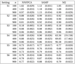
errors are reported in parentheses. . . 78 Table 4.2 AverageL2_{difference between the estimated and true mean functions.}

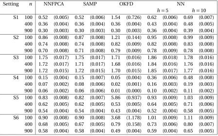
Standard errors are reported in parentheses. M2 refers to the second methods proposed in Gromenko et al. (2012). . . 79 Table 4.3 AverageL2_{difference between predicted and true curves for new}

lo-cations. Standard errors included in parentheses. . . 80 Table 4.4 AverageL2_{difference in estimated and true FPCs for noisy data.}

(12)

Table 4.5 AverageL2_{difference in estimated and true mean functions for noisy} data. Standard errors are reported in parentheses. M2 refers to the second methods proposed in Gromenko et al. (2012). . . 85 Table 4.6 AverageL2_{difference between predicted and true underlying smooth}

curves for new locations. Standard errors included in parentheses. . . 86 Table A.1 Maximum likelihood estimates of the spatiotemporal covariance

pa-rameters separated by network and direction for sulfate. Standard errors for the estimates are found below in parentheses. Values de-noted with an asterisk are rounded to zero, but their estimated values are not zero. . . 106 Table A.2 Average daily MSE and MAD of all folds on the log-scale and

orig-inal scale for our method (ST-FDA), k-nearest neighbors approach (kNN) and spatiotemporal Kriging (STK) under two settings of missing observations . . . 109 Table A.3 Average MSE of seasonal site averages on the log-scale and original

scale for our method (ST-FDA), nearest neighbors approach (kNN) and spatiotemporal Kriging (STK) under two settings of missing ob-servations. . . 110 Table A.4 90% prediction interval coverage for seasonal average predictions

on the log-scale with corresponding standard errors listed below in parentheses. . . 110 Table A.5 Comparison of how our approach and other methods account for

features of the current PM_2.5data set. . . 115 Table A.6 Covariance model AICs for nitrate. . . 116 Table A.7 Covariance model AICs for sulfate. . . 116 Table A.8 MSE of seasonal site averages on the log-scale and original scale for

our method (ST-FDA), nearest neighbors approach (kNN) and spa-tiotemporal Kriging (STK) under two settings of missing observations.

. . . 116 Table A.9 MAD of seasonal site averages on the log-scale and original scale for

our method (ST-FDA), nearest neighbors approach (kNN) and spa-tiotemporal Kriging (STK) under two settings of missing observations.

. . . 117 Table A.10 Average MAD of seasonal site averages on the log-scale and original

(13)

Table A.13 Maximum likelihood estimates of the spatiotemporal covariance pa-rameters separated by pollutant and direction for nitrate. Standard errors for the estimates are found below in parentheses. Values de-noted with an asterisk are rounded to zero, but their estimated values are not zero. . . 121 Table A.14 Average nitrate daily prediction MSE and MAD on the log-scale and

original scale for the separate and joint models under two settings of missing observations. . . 122 Table A.15 Average sulfate daily prediction MSE and MAD on the log-scale and

original scale for the separate and joint models under two settings of missing observations. . . 122 Table A.16 Average daily prediction MSE for the regional and national analyses

on the log-scale. . . 123 Table A.17 Average daily prediction MAD for the regional and national analyses

on the log-scale. . . 124 Table B.1 Size results forn =200 andm =25 from 5000 simulation replicates. . 132 Table B.2 Size results forn =400 andm =15 from 5000 simulation replicates. . 133 Table B.3 Size results forn =400 andm =25 from 5000 simulation replicates. . 133 Table B.4 One test size results forn=200, andm=25 for data generated from

non-normal scores under Scenario 2. Results are from 5000 simulation replicates. Values in bold are more than two standard errors above the nominal size. . . 137 Table B.5 One test size results forn=400, andm=15 for data generated from

non-normal scores under Scenario 2. Results are from 5000 simulation replicates. Values in bold are more than two standard errors above the nominal size. . . 137 Table B.6 One test size results forn=400, andm=25 for data generated from

(14)

LIST OF FIGURES

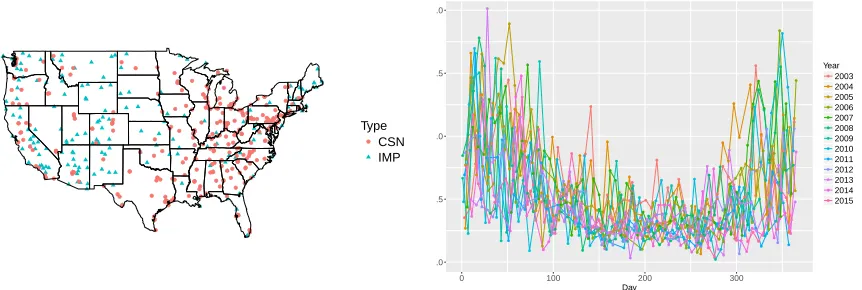
Figure 2.1 The left panel shows the location of the sites in the two networks: IM-PROVE (blue triangles) and CSN (red circles). The right panel depicts the data for a CSN site in North Carolina observed from 2003-2015. . 12 Figure 2.2 Left panel: estimated mean functionµ(_b d)corresponding to CSN (red)

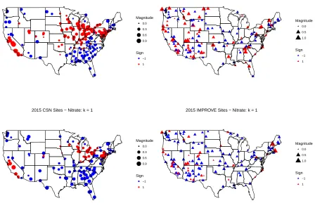
and IMPROVE (blue). Results are shown on the log-scale. Middle and right panels: estimated eigenfunctions for nitrate variation,φÒ_k(d), for CSN sites (middle, K=3) and IMPROVE sites (right, K=3). . . 18 Figure 2.3 Preliminary predicted loadings for the first direction for nitrate

varia-tion in 2003 (top panels) and 2015 (bottom panels): CSN sites (left panels) and IMPROVE sites (right panels). . . 22 Figure 2.4 Observed and estimated nitrate levels on the log-scale for a CSN site

in Alabama from 2003 to 2006 (from left to right). . . 26 Figure 2.5 Estimated random slopes for the first direction of nitrate variation

for CSN sites (left panel) and IMPROVE sites (right panel). . . 30 Figure 2.6 Annual (top panels) and seasonal (middle and bottom panels)

av-erage total (nitrate+sulfate) pollution levels for each state for 2003 and 2015 for CSN. Totals are on the log-scale. The sections of the pie represent the proportion of the total pollution accounted for by each pollutant. The radius of the circle represents the level of total pollu-tion and is scaled appropriately so we can compare levels between the years and seasons. . . 34 Figure 2.7 Annual (top panels) and seasonal (middle and bottom panels)

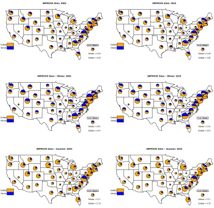
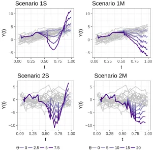
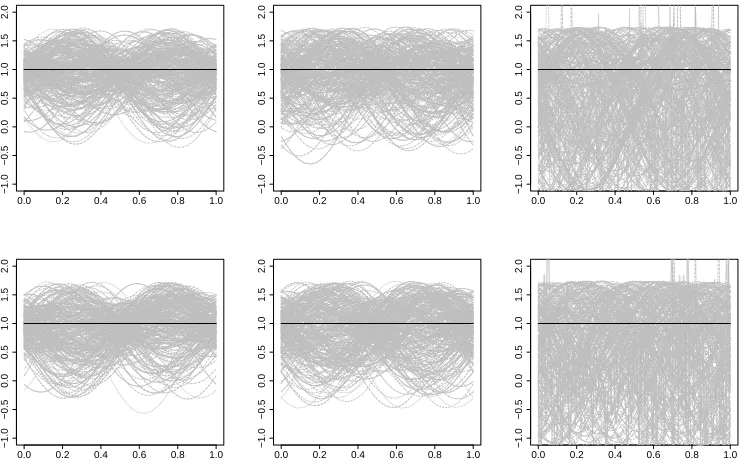
av-erage total (nitrate+sulfate) pollution levels for each state for 2003 and 2015 for IMPROVE. Totals are on the log-scale. The sections of the pie represent the proportion of the total pollution accounted for by each pollutant. The radius of the circle represents the level of total pollution and is scaled appropriately so we can compare levels between the years and seasons. . . 35 Figure 3.1 Displayed is a sample of 20 curves (gray solid lines) corresponding to

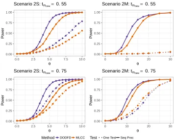
Scenario 1 (top panels) or Scenario 2 (bottom). Overlayed in purple-color are curves that deviate from the overall pattern starting atu= 0.5 corresponding to a Shape deviation (left panels) or a Magnitude deviation (right), where the amount of deviation is controlled byθ. 49 Figure 3.2 Power performance of both DODFD and MLCC corresponding to

significance levelα=0.01. Results are presented for Scenario 2,n= 200 andm =15 and are based on 1000 simulation replicates. Here tmn e w indicates the time point for the single test as well as the starting

(15)

Figure 3.3 Left panel: depicted on log scale are the pace trajectories (gray lines) of the 788 female runners from 2014 TCS NYC marathon that form the apriori sample and their mean trajectory (black dashed line). Overlaid in black solid lines are the pace trajectories for the runners with the slowest 10% marathon time performance at the 2015 TCS NYC marathon. Right panel: the estimated top three FPCs of the apriori sample pace trajectories. . . 57 Figure 3.4 Depicted in gray lines are the pace trajectories of the bottom 10%

per-formance time at marathon 2015 TCS NYC marathon; black dashed line shows the mean pace trajectory based on the 2015 TCS NYC marathon apriori sample. Overlaid in purple color are the outlying trajectories identified with DODFD (left panel) and in orange color are the outlying trajectories identified with MLCC (right panel). The change from dark to light (purple or orange) indicates the distance at which a runner was detected. . . 58 Figure 4.1 Estimated FPCs are shown in grey lines, and the true FPC is

repre-sented with the black line fork =1 (left panel) andk =2 (right panel). 65 Figure 4.2 Sampling design of an upright square lattice and distances between

neighboring sites. . . 67 Figure 4.3 Estimatedφ_k(t)fork=1 under Setting S1 for NNFPCA (left column),

SAMP (middle column) and M2 from Gromenko et al. (2012) (right column). The first row displays the estimates forn =100 and the second row contains the estimates forn=900. Results fork =2, 3 are located in Section C.3 of the Appendix. . . 76 Figure 4.4 Estimatedφ_k(t)fork=1 under Setting S4 for NNFPCA (left column),

SAMP (middle column) and M2 from Gromenko et al. (2012) (right column). The first row displays the estimates forn =100 and the second row contains the estimates forn=900. . . 77 Figure 4.5 Estimatedµ(t)under Setting S1 for NNFPCA (left column), SAMP

(middle column) and M2 from Gromenko et al. (2012) (right column). The first row displays the estimates forn=100 and the second row contains the estimates forn=900. . . 81 Figure 4.6 Estimatedφk(t)fork=1 under Setting S1 withS N R=10 for

NNF-PCA (left column), SAMP (middle column) and M2 from Gromenko et al. (2012) (right column). The first row displays the estimates for n=100 and the second row contains the estimates forn =900. . . . 83 Figure 4.7 The left panel depicts the monitoring locations in the data set and

(16)

Figure 4.8 From left to right the estimated mean functions, and 3 estimated FPCs found using the NNFPCA and SAMP methods. The NNFPCA es-timates are represented with the solid lines, and the SAMP eses-timates are shown in the dashed lines. . . 88 Figure A.1 Left panel: estimated mean functionµ(_b d)corresponding to CSN (red)

and IMPROVE (blue) for sulfate. Results are shown on the log-scale. Middle and right panels: estimated eigenfunctions for sulfate varia-tion,φÒ_k(d), for CSN sites (middle) and IMPROVE sites (right). . . 106 Figure A.2 Preliminary predicted loadings for the first direction for sulfate

varia-tion in 2003 (top panels) and 2015 (bottom panels): CSN sites (left panels) and IMPROVE sites (right panels). . . 107 Figure A.3 Observed and estimated log-sulfate levels for a CSN site in Alabama

from 2003 to 2006 (from left to right). . . 108 Figure A.4 Estimated random slopes for the first direction of sulfate variation

for CSN sites (left panel) and IMPROVE sites (right panel). . . 111 Figure A.5 Sample directional semivariograms fork =1 in 2003 for CSN sites

(left panel) and IMPROVE sites (right panel). Directions are in degrees.112 Figure A.6 Sample directional semivariograms fork =1 in 2003 for CSN sites

(left panel) and IMPROVE sites (right panel). Directions are in degrees.113 Figure A.7 The six regions of the U.S. used for regional model fitting. . . 123 Figure B.1 Power of tests at anα = 0.01 significance level for selected tmn e w.

Data is generated from Scenario 2 withn=200 andm=25 for 1000 simulation replicates. . . 134 Figure B.2 Power of tests conducted with anα=0.01 significance level for

se-lected values oftmn e w. Data is generated under Scenario 1 forn=200

andm=15 with 1000 simulation replicates. . . 135 Figure B.3 Power of tests at anα = 0.01 significance level for selected tmn e w.

Data is generated from Scenario 1 withn=200 andm=25 for 1000 simulation replicates. . . 136 Figure C.1 Sampling design of an upright square lattice and distances between

neighboring sites. . . 145 Figure C.2 NNFPCAφk(t)estimates fork =1 (left),k =2 (center) andk =3

(right) forN =100 simulation replicates of sizen=22, 500. . . 146 Figure C.3 Estimatedφ_k(t)fork=2 in the left 2 columns (NNFPCA on the left,

(17)

Figure C.4 NNFPCAφ_k(t)estimates fork =1 (left),k =2 (center) andk =3 (right) under Setting S2. The first row corresponds to the case where n=100 and the second row ton =900. . . 148 Figure C.5 NNFPCAφk(t)estimates fork =1 (left),k =2 (center) andk =3

(18)

CHAPTER

1 INTRODUCTION

Functional data analysis (FDA) is an area of statistics in which the response of interest is a function rather than a univariate value. For example, one of the Environmental Protection Agency’s (EPA) fine particulate matter data sets, which will be formally introduced in Chap-ter 2, features measurements of nitrate taken every third day over the course of a year. In univariate statistics, the focus would be on nitrate levels on a single day, whereas in FDA the goal is to understand the behavior of nitrate levels throughout the year. FDA assumes there is a smooth but unknown underlying process generating the discretely observed measurements and seeks to understand this process. Thanks to advances in computing capabilities, FDA has grown in popularity, and many statistical techniques developed for univariate or multivariate data have been modified and extended to the functional data realm. Additionally, new methods have been introduced to study problems unique to func-tional data. For a thorough overview of FDA see Ramsay and Silverman (2002), Ramsay and Silverman (2005a) and Horváth and Kokoszka (2012), among others.

Consider a general sample of functional data_{(Yi j,ti j):i =1, . . . ,n;j =1, . . . ,mi}where

(19)

is a closed compact set. As a concrete example,Yi j could be the level of nitrate measured at

locationion dayti jin the fine particulate matter data set. FDA considers theYi jvalues to be

realizations of a smooth but unknown underlying random processX(·)that are potentially observed with error. Therefore, functional data are commonly represented as

Yi j=Xi(ti j) +εi j (1.1)

whereXi(·)is the realization of the process for subject (or curve)i, andεi j are independent

and identically distributed (i.i.d.) errors with mean zero and varianceσ2_{. It is assumed} thatX(·)is a square integrable function inL2₍_T₎₍R

T E{X

2₍_t₎_}_{d t} _<_∞_{) with smooth mean} functionE{X(t)}=µ(t)and smooth covariance functionC o v{X(t),X(t0₎_}₌_Σ₍_t_,_t0₎_.

Traditionally, FDA has considered_{ti1, . . . ,ti mi}to be densely observed inT at regular

sampling points for alli; this is referred to as dense functional data. However, many FDA methods also consider problems in which the set_{ti1, . . . ,ti mi}is sparsely and irregularly

sampled inT with the assumption that{ti1, . . . ,ti mi :i =1, . . . ,n}is dense inT. In other

words, each subject or curve has a small number of measurements, and the sampling points differ acrossi. However, the complete set of sampling points for all curves is dense in_T . This second scenario is known as sparse functional data.

Although the rise of FDA has yielded many new statistical methods for both dense and sparse functional data, most FDA methods were developed under the assumption of an independent sample of functional data. However, for more complex data sources, it may be inappropriate to assume that the curves are independent. For example, the nitrate measurements in the fine particulate matter data set studied in Chapter 2 are recorded at various locations throughout the U.S. for multiple years, and it is reasonable to assume that the nitrate levels are spatially correlated across locations. In addition, if the annual nitrate profiles measured for multiple years are considered to be repeated functional observations at each site, then there is likely correlation across years as well. This perspective allows the cyclic behavior of pollutant levels across years to be leveraged in analysis.

(20)

Similarly, Greven et al. (2010), Chen and Müller (2012) and Park and Staicu (2015) studied longitudinal functional data.

Improvements in technology also allow for data to be monitored as they are being observed or in real-time. For example, wearable fitness trackers now generate real-time data, such as heart rates or speeds, throughout exercise or athletic competitions. In this setting, it would be beneficial to identify potential deviations from typical behavior to help users, coaches or competition organizers make decisions. Indeed, identifying a marathon runner whose speed decreases sharply during the race could help race organizers provide prompt medical attention if the runner is suffering from dehydration or heat exhaustion. These types of repeated responses over time lend themselves to a functional data per-spective, but there has been limited research into FDA methods for real-time outlier de-tection problems. Most outlier dede-tection methods in FDA instead seek to identify outlying curves from a static sample of functional data. Febrero et al. (2008), Sun and Genton (2011), Gervini (2012) and Arribas-Gil and Romo (2014) considered measures of functional depth to identify outliers. Another set of approaches utilized functional principal component analysis (FPCA) to identify curves that deviate noticeably in one of the main directions of variation in the sample of functional data (Hyndman and Shang, 2010; Yu et al., 2012).

(21)

1.1 Contributions and outline

In Chapter 2, we propose a modeling approach to accommodate spatial and temporal dependence in functional data observed at various spatial locations over time. This method is developed to analyze fine particulate matter monitored across multiple years at sites across the country. To incorporate likely periodicity across years in the data, we view the responses at each site as a functional time series. We model the data using an overall mean function, a linear combination of smooth within-year trends and site/year-specific coefficients, and a residual error term. We use FPCA to estimate the smooth within-year trends and then model the dependence across space and years through the site/ year-specific coefficients. This approach reduces the dimensionality of the problem, allowing for easier visualization and in turn better understanding of the complex trends and variation in the data. Additionally, it yields faster computation in comparison to Bayesian hierarchical modeling approaches developed for similar data sets. Finally, the considered data set features locations that are missing entire years or large portions of measurements within a given year. Our modeling approach allows us to predict missing years or impute portions of years for those sites as well as to predict complete trajectories for unmonitored locations. While this method was developed for application to the fine particulate matter data set, it can also be applied to similar data sets consisting of repeated functional responses measured across various spatial locations.

(22)

goal of detecting participants who deviate from typical race pacing.

The main objective of Chapter 4 is to develop an FPCA estimation procedure for spatially correlated functional data that are observed in a fixed domain. In this chapter, we assume the data are dense and fully observed without noise and discuss an extension to data observed with noise. Unlike in the case of independent data, estimators from spatially correlated data in a bounded spatial domain are not generally consistent when the number of spatial locations increases to infinity (Lahiri, 1996; Stein, 2010). This is also true of FPCs (Hörmann and Kokoszka, 2013). We propose a novel method to estimate FPCs in this context that yields consistent estimates under certain assumptions. Our approach is inspired by an alternative representation of the sample covariance, which is expressed in terms of pairwise differences. For a given location, we take a weighted average of the differences between the curve at the current location and the curves corresponding to the location’s nearest spatial neighbors. We take a simple average of the site-specific weighted averages across sites and spectrally decompose this quantity to estimate the FPCs. Although the key contribution of this chapter is significantly improved FPC estimation, we also use the FPCs to estimate the mean function and to predict trajectories for unobserved locations. Through simulations, we illustrate the significant improvement of our FPC estimates in comparison to other methods, even in settings in which the conditions for consistency are violated. We also find that our mean estimation and new location prediction approaches are generally preferred, or at least comparable, to competing methods for various settings of spatial dependence. We apply our method to a subset of the previously studied fine particulate matter data set to investigate if we find similar within-year trends in nitrate levels to those found in Chapter 2.

Based on the results in Chapters 2 - 4, Chapter 5 briefly discusses potential areas of future work. The methods in Chapters 2 - 4 rely on common FDA techniques including smoothing and FPCA. We conclude this introduction with a brief overview of these methods.

1.2 Smoothing functional data

(23)

domain in order to characterize the infinite-dimensional data generating process. Many smoothing approaches have been proposed including kernel smoothing (Wand and Jones, 1995), local polynomial smoothing (Fan and Gijbels, 1996; Zhang, Chen, et al., 2007) and penalized basis expansions (see Wahba 1990; Ruppert et al. 2003; Wood 2006 and others). In Chapter 4, we utilize a penalized basis expansion approach, specifically using b-spline and Fourier bases, and we briefly describe this approach next.

Consider model (1.1) for the functional data, and assume the sampling points for each curve are dense in_T. The goal of smoothing is to use a linear combination of coefficients and the selected basis to describe{Yi j :j =1, . . . ,mi}. Specifically, let{B1(t), . . . ,BL(t)}be

the considered basis of dimensionL. This basis and a set of subject-specific coefficients {β1i, . . . ,βLi}are used to approximate the observed data as XÒ_iL(t) =

PL

`=1β`iB`(t)for all

i. The goal is to find basis coefficients that minimize the sum of squared errors,SS E = Pmi

j=1{Yi j−XÒ_iL(t_{i j})}2.

It is clear that the larger the dimension of the basis, the better the representation of the data. Indeed, ifL=mi, then the observed data can be perfectly interpolated. However, as the

goal is to smooth out noise in the data, we do not want to perfectly fit each curve. Therefore, the objective function is modified by including a penalty term that is used to control the balance between the goodness of fit and the smoothness of fit:P SS E_λ=SS E+λP{XÒ_iL(·)} whereP{·}is the penalty term, andλis a smoothing parameter. A common and natural choice for this penalty isP{XÒ_iL(·)} =

R T{XÒ

L00

i (t)}

2_{d t} _where _f 00₍_t₎_{represents the second} derivative of a function f(t). Following from the basis representation ofXÒ_iL(t), this term becomesP{XÒ_iL(·)}=

PL

`=1

PL

`0₌1β`iβ`0_i

R T B

00

`(t)B`00(t)d t. Ifλ=0, then theP SS Eλis simply

the standardSS E. Therefore, smaller values ofλcorrespond to more “wiggly” fits, and larger values ofλwill result in more linear representations of the curves.

(24)

1.3 Functional principal component analysis

Functional principal component analysis is a key tool in FDA, and it is utilized throughout the following chapters of this dissertation. We briefly discuss the general approach for FPCA and then address estimation methods in the context of dense and sparse functional data. For more detail on FPCA for dense functional data see Rice and Silverman (1991), Hall and Hosseini-Nasab (2005), and Yao et al. (2005b) among others, and for sparse functional data see Staniswalis and Lee (1998), James et al. (2000), Yao et al. (2005a), and Peng and Paul (2009).

As a reminder, we assume theYi js are noisy realizations of a smooth, square integrable

processX(·)with smooth mean functionµ(t)and smooth covariance functionΣ(t,t0₎_. Fol-lowing from these assumptions, Mercer’s lemma (Mercer, 1909) yields a spectral decompo-sition of the covariance; specifically,Σ(t,t0) =P_k_≥1λkφk(t)φk(t0)where theλksare

eigen-values satisfyingλ1> λ2>· · · ≥0, and theφk(·)s are orthonormal eigenfunctions inL2(T)

whereR

Tφk(t)φk0(t)d t =1 ifk=k

0_{and 0 otherwise. Following from the Karhunen-Loève} (K-L) expansion (Loève, 1945; Karhunen, 1947) the data can be optimally represented in terms of the eigenbasis asXi(t) =µ(t)+

P

k≥1ξi kφk(t)whereξi k=

R

T{Xi(t)−µ(t)}φk(t)d t, and these basis coefficients are random with zero mean and varianceλ_k. It is further assumed that these coefficients are independent acrossk.

When adopting this representation, we assume that a finite truncation of the K-L ex-pansion can well approximateXi(·), sayX_iK(t) =

PK

k=1ξi kφk(t)for someK. Much like the selection of the smoothing parameter in penalized basis expansions, there are many meth-ods to choose this truncationK including Akaike information criterion (AIC) (Yao et al., 2005a) or Bayesian information criterion (BIC) (Li et al., 2013). Another approach, which we utilize in this dissertation, is to selectK based on a threshold for the percentage of variation explained (PVE) by the leadingK components (see Di et al. 2009, James et al. 2000, Staicu et al. 2010 and others).

Estimation of the model parameters specified above differs for dense and sparse func-tional data. In the case of a dense sampling design, the curves are individually pre-smoothed using a chosen smoothing method. This yields smooth, fully observed trajectories, say

e

Xi(t), for each i, and the smooth mean function is estimated using the sample mean,

b

µ(t) = _n1Pn

i=1Xei(t). The covariance function is estimated using the detrended smooth

data asΣb(t,t0) = 1

n−1 Pn

i=1{Xei(t)−µ(b t)}{Xei(t 0₎₋

b

(25)

b

Σ(·,_·)yields the estimated eigenfunctionsφÒ_k(·)and eigenvaluesλb_k fork =1, . . . ,K. The coefficients are then estimated asξb_{i k}=

R

T{Xei(t)−µ(b t)}φÒk(t)d t where the integral is ap-proximated through numerical integration.

For sparse functional data, pre-smoothing each curve individually is unreliable due to the small number of measurements for eachi. Instead, the curves are pooled to estimate

b

µ(·)andΣb(·,·)(Yao et al., 2005a). A univariate smoothing technique is first applied to{Yi j :

i =1, . . . ,n;j =1, . . . ,mi}to estimateµ(·), and the curves are detrended asYei j=Yi j−µ(tb i j). Next a raw estimate of the sample covariance is constructed using the pairwise products Ci j j0=Yi jYi j0for all pairs(ti j,ti j0), and a bivariate smoothing technique, such as bivariate local polynomial smoothing (Eilers and Marx, 2003) or thin plate regression splines (Wood, 2003), is utilized to estimateΣb(t,t0). Due to noise in the data,E(C_{i j j}0) =Σ(t_{i j},t_{i j}0)+σ2I(j= j0₎_{, and thus there is bias on the diagonal of the raw covariance. Therefore, most common} bivariate smoothing approaches remove the diagonal elementsCi j j prior to smoothing, and

σ2_{is later estimated by applying a univariate smoother to the differences in the diagonals} Ci j j−Σb(ti j,ti j).

The estimates of the eigenfunctions and eigenvalues can be recovered through the spectral decomposition of the smooth estimated covariance. With sparse functional data, the random basis coefficients cannot be estimated through numerical integration. Instead, Yao et al. (2005a) proposed the use of a conditional expectation to estimate the scores b

ξi k =E[ξi k|Yi]whereYi= (Yi1, . . . ,Yi mi)

T _{is the vector of measurements of curve}_i_{. These}

es-timated coefficients are the best linear unbiased predictors if theξ_{i k}andε_{i j}are jointly Gaus-sian. In this case, the conditional expectation further simplifies toξb_{i k} =bλ_kφÒ_{i k}TΣb−1_Y

i(Yi−µbi)

whereµ_b_iandφÒ_{i k} are the vectors of estimated model components evaluated at{t_i₁, . . . ,t_{i m}

i}

and similarlyΣbYi is themi×mi estimated covariance matrix ofYi.

(26)

CHAPTER

2 A FUNCTIONAL DATA ANALYSIS OF

SPATIOTEMPORAL TRENDS AND

VARIATION IN FINE PARTICULATE

MATTER

2.1 Introduction

(27)

to visibility degradation through the scattering and absorption of visible light (Malm et al., 2004) and excessive nutrient and pollutant deposition.

In this chapter we are concerned with characterizing how two main pollutant species of PM_2.5- particulate nitrate (NO−

3) and particulate sulfate (SO−24 ) - vary during 2003-2015 across the U.S. The motivating data set contains concentrations of these pollutant species recorded by two monitoring networks, which operate independently and often have dis-parate sampling protocols and standard operating procedures; see Figure 2.1. Our objective is to study the variability of fine particulate nitrate and sulfate over time and across the U.S. using recent functional data analysis techniques.

Due to the health risks and visibility degradation associated with high concentrations of PM_2.5, its behavior has been extensively studied. Millar et al. (2010) provide a thorough review of approaches to modeling exposure to fine particulate matter. A popular class of methods are empirical (statistical) methods, common examples of which include Kriging (see Liao et al., 2006 and Leem et al., 2006 among others) and land use regression mod-els. Hoek et al. (2008) provide a review of various land use regression models utilized to investigate spatial variation in concentrations. Physical models, which apply mathematical equations from physical processes, are another common approach (Cyrys et al., 2005; Næss et al., 2007). Finally, many hybrid methods have been developed to incorporate different models and data sources (Hu et al., 2013; Liu et al., 2009). Berrocal et al. (2009) provide a way to incorporate data with different spatial supports; they use their method to analyze ozone levels using measurements taken from specific monitoring locations and the Community Multiscale Air Quality (CMAQ) model.

(28)

et al. (2011) consider data with a similar structure to ours and propose a spatiotemporal model that separates temporal trends and spatially varying coefficients and allows for non-stationary spatial correlation. Table A.5 in Appendix A provides further comparison of these approaches.

The use of functional data analysis methods for environmental data has received at-tention recently (Gao and Niemeier, 2008; Park et al., 2013; Shaadan et al., 2012; Hörmann et al., 2015). We propose incorporating the annual periodicity of the measurements into the model by viewing the annual concentration profiles at a location as afunctional time

series(Hörmann and Kokoszka, 2012) and modeling it as the sum of three components: 1)

an annual mean level, 2) a linear combination of smooth annual trends with site-specific coefficients that vary over the years during the period of study, and 3) an annual specific residual effect. The annual trajectory may or may not vary over the space, and the annual residual profile is assumed to be independent across sites and years, but allowed to exhibit dependence within a year. Although derived from a different perspective, our modeling technique shares several similarities with Sampson et al. (2011). Both approaches rely on a linear combination involving orthogonal smooth temporal trends. Sampson et al. (2011) worked with the full time series and the temporal trends were functions defined over the entire period under study. In contrast, we view the site level data as afunctional time series

where the functional argument isday within yearand the series is indexed byyear, and thus the trends are functions defined over a year-time. As a consequence of the different perspectives, the coefficients were space-dependent solely in Sampson et al. (2011), while they exhibit both spatial and yearly variation in the proposed approach. Furthermore the assumptions of the residual process are different: the residual component was allowed to have spatial dependence and was assumed independent over days/years in Sampson et al. (2011), while it is allowed to have dependence across the days within year but is assumed independent over space and years in our method.

(29)

struc-ture - such as separable covariance strucstruc-tures which assume the dependence across space is independent of time and vice versa - are often needed to make computation feasible. By comparison, the proposed method considers a non-separable and non-stationary covari-ance structure. Third, the proposed method allows us to better visualize and gain insights from the data.

The remainder of the chapter is structured as follows: Section 2.2 describes the data to be used in this chapter. The modeling framework and estimation techniques are detailed in Section 2.3. The application of the proposed methods to our data and interpretation of the results are discussed in Section 2.4, and a description of the software implementation is found in Section 2.5. We conclude with a brief summary in Section 2.6.

2.2 Data description

Particulate nitrate and sulfate are recorded by two networks: the Interagency Monitoring of Protected Visual Environments (IMPROVE), and the Chemical Speciation Network (CSN).

● ● ●● ● ● ● ● ● ● ● ●● ● ● ● ● ●● ● ● ● ● ● ● ● ● ● ●● ● ● ● ● ● ● ● ● ● ● ● ● ●●● ● ● ● ● ● ● ● ●● ● ● ● ● ● ● ● ● ● ● ● ● ● ● ● ● ● ● ● ● ● ● ● ● ● ● ● ● ● ● ● ● ● ● ● ● ● ● ● ● ● ● ●●●●● ● ● ● ● ● ● ● ●● ● ● ● ● ● ● ● ● ● ● ● ●●●● ● ● ● ● ● ● ● ● ● ● ● ● ● ● ●● ● ● ● ● ● ● ● ● ● ● ● ● ● ●● ● ●● ●● ● ● ● ● ● ● ● ● ● ●● ● ● ● ● ● ● ●● ● ●● ● ● ● ● ● ● ● ● ● ● ● ● ● ● ● ● ● ● ● ● ● ● ● ● ● ● ●● ● ● ● ● ● ● ● ● ● ● ● ●●●●●● ● ● ● ● ● ● ●● ● ● ● ● ●● ● ● ● ● ● ● ● ● ● ● ● ● ● ● ● ● ● ● ● ● ●● ● ● ● ● ● ● ● ● ● ● ● ●● ●● ● ● ● ● ● ● ● ● ● ● ● ● ● ● ●● ● ● ● ● ● ● ● ● ● ● ● ● ● ●● ● ● ● ● ● ● ● ● ● ● ● ● ● ● ● Type ● _CSN IMP ● ● ● ● ● ● ● ● ● ● ● ● ● ● ● ● ● ● ● ● ● ● ● ● ● ● ● ● ● ● ● ● ● ● ● ● ● ● ● ● ● ● ● ● ● ● ● ● ● ● ● ● ● ● ● ● ● ● ● ● ● ● ● ● ● ● ● ● ● ● ● ● ● ● ● ● ● ● ● ● ● ● ● ● ● ● ● ● ● ● ● ● ●● ● ● ● ● ● ● ● ● ● ● ● ● ● ● ● ● ● ● ● ● ● ● ● ● ● ● ● ● ● ● ● ● ● ● ● ● ● ● ● ● ● ● ● ● ● ● ● ● ● ● ● ● ● ● ● ● ● ● ● ● ● ● ● ● ● ● ● ● ● ● ● ● ● ● ● ● ● ● ● ● ● ● ● ● ● ● ● ● ● ● ● ● ● ● ● ● ● ● ● ● ● ● ● ● ● ● ● ● ● ● ● ● ● ● ● ● ● ● ● ● ● ● ● ● ● ● ● ● ● ● ●● ● ● ● ● ● ● ● ● ● ● ● ● ● ● ● ● ● ● ● ● ● ● ● ● ● ● ● ● ● ● ● ● ● ● ● ● ● ● ● ●● ● ● ● ● ● ● ●● ● ● ● ● ● ● ● ● ● ● ● ● ● ● ● ● ● ● ● ● ● ● ● ● ● ● ● ● ● ● ● ● ● ● ● ● ● ● ● ● ● ● ● ● ● ● ●● ● ● ● ● ● ● ● ● ● ● ● ● ● ● ● ● ● ● ● ● ● ● ● ● ●● ● ● ● ● ● ● ● ● ● ● ● ● ● ● ●● ● ● ● ● ● ● ● ● ● ● ● ● ● ● ● ● ● ● ● ● ● ● ● ● ● ● ● ●● ● ● ● ● ● ● ● ● ● ● ● ● ● ● ● ● ● ● ● ● ● ● ● ● ● ● ● ● ● ● ● ● ● ● ● ● ● ● ● ● ● ● ● ● ● ● ● ● ● ● ● ● ● ● ● ● ● ● ● ● ● ● ● ● ● ● ● ● ● ● ● ● ● ● ● ● ● ● ● ● ● ● ● ● ● ● ● ● ● ● ● ● ● ● ● ● ● ● ● ● ● ● ● ● ● ● ● ● ● ● ● ● ● ● ● ● ● ● ● ● ● ● ● ● ● ● ● ● ● ● ● ● ● ● ●● ● ● ● ● ● ● ● ● ● ● ● ● ● ● ● ● ● ● ● ● ● ● ● ● ● ● ● ● ● ● ● ● ● ●● ● ● ● ● ● ● ● ● ●● ● ● ● ● ● ● ● ● ● ● ● ● ● ● ●● ● ● ● ● ● ● ● ● ● ● ●● ● ● ● ● ● ● ● ● ● ● ● ● ● ● ● ● ● ● ● ● ● ● ● ● ● ● ● ● ● ● ● ● ● ● ● ● ● ● ● ● ● ● ● ● ● ● ● ● ● ● ● ● ● ●● ● ● ● ● ● ● ● ● ● ● ● ● ● ● ● ● ● ● ● ● ● ● ● ● ● ● ● ● ● ● ● ● ● ● ● ● ● ● ● ● ● ● ● ● ● ● ● ● ● ● ● ● ● ● ● ● ● ● ● ● ● ● ● ● ● ● ● ● ● ● ● ● ● ● ● ● ● ● ● ● ● ● ● ● ● 0.0 0.5 1.0 1.5 2.0

0 100 200 300

Day Year ● ● ● ● ● ● ● ● ● ● ● ● ● 2003 2004 2005 2006 2007 2008 2009 2010 2011 2012 2013 2014 2015

Figure 2.1 The left panel shows the location of the sites in the two networks: IMPROVE (blue

triangles) and CSN (red circles). The right panel depicts the data for a CSN site in North Carolina observed from 2003-2015.

IMPROVE. The IMPROVE network, which began operations in 1985, represents a

(30)

the sites are depicted using filled triangles in Figure 2.1. They collect 24-hour integrated samples every third day (midnight to midnight LST). For a detailed description, see Malm et al. (2004).

CSN. The U.S. EPA’s more recently established CSN also follows the one-in-three days collection protocol; see the CSN website for more information (EPA, 2016). Most of the sites monitored by this network are located in urban areas with a greater density in the eastern U.S.; the sites are depicted using filled circles in Figure 2.1.

Our study is limited to the period 2003-2015. In spite of the one-in-three day planned sampling schedule, several sites had no data for some years, or if they had observations during a year, they had only a few, in some cases covering less than a half a year period. A few CSN sites had multiple non-consistent recordings for sulfate during the same year and none for nitrate; those CSN sites during the respective years were omitted from the analysis. Our analysis is based on the remaining sites: 184 IMPROVE sites and 326 CSN sites. Most of these contain pollutant measurements for all 13 years; however there are sites observed only one year during this time frame, a few years but not necessarily consecutive years, or they had very sparse recordings during a year. Some analyses of similar data sets have utilized weekly or biweekly averages to handle missing daily measurements (Smith et al., 2003; Sahu et al., 2006; Sampson et al., 2011). However, daily PM2.5measurements are often used in studies as predictors for negative health outcomes (Bell et al., 2004; Dominici et al., 2006; Zanobetti et al., 2009). In these situations, daily predictions for missing days would be beneficial. Further, by utilizing data on the daily scale we can avoid averaging over potentially unequal numbers of daily measurements.

(31)

2.3 Modeling framework

Environmental data often has a complex spatiotemporal dependence structure and mod-eling it poses many challenges. Let Yi j(d) be the response (log-transformed nitrate or

sulfate concentration) at sitei, year 13ti j for ti j ∈ {1/13, 2/13, . . . , 1}, day 365d, ford ∈

{1/365, 2/365, . . . , 1_}, and letsi be the latitude/longitude of sitei. We scaleti j andd so they

are both within the[0, 1]interval. Asd is a function of the day within year, we will often refer tod by day, with the understanding that the actual day within year is 365d. Similarly, we will refer toti j by year, corresponding to the years of study from 2003 to 2015, even though

the true year is 13ti j+2002. We posit the following model

Yi j(d) =µ(d,si,ti j) +

P

k≥1ξk i jφk(d) +εi j(d); (2.1)

whereµ(d,si,ti j)is the mean function which can depend on site, year or day specific

covari-ates, the sum-term in the middle is the site-specific deviation from the overall mean and will be detailed next, andε_{i j}(_·)is the site/time specific deviation. The termP_k_≥1ξ_{k i j}φ_k(d) is a linear combination of year-time functionsφk(·)that are assumed invariant across years

and mutually orthogonal, in the sense thatR₀1φk(u)φk0(u)d u=1 ifk =k0and 0 otherwise. The basis coefficientsξk i j quantify the dynamic variation over space (si) and time (ti j)

corresponding to the annual pattern represented byφk(·). It is assumed that the

spatiotem-poral processξk(si,ti j) =ξk i j is independent from the noise measurementεi j(·)for allk.

Also for convenience we assume that theξ_{k i j}s are independent acrossk. In practice we use a finite truncationK so that in model (2.1) the summation is fork=1, . . . ,K. Finally, we assume thatε_{i j}(d)is the zero mean measurement error that is independent acrossi and j but possibly dependent overd.

The model in (2.1) is inspired from Park and Staicu (2015) in the way it models the dynamic behavior over time using time-invariant orthogonal basis functions. Nevertheless, (2.1) is different from Park and Staicu (2015), who assume that the time varying curvesYi j(·)

are independent overi and thus are solely dependent over j. We assume thatξk i j vary

according to the following model

ξk i j =ak i+ti jbk i+ek i j, (2.2)

(32)

and sitesi, andek i j is a nugget effect with variance denoted byσk2. We assume thatak i

andbk i are independent Gaussian processes overk and furthermore are mutually

inde-pendent; to account for the dependence of the curves over sites, it is assumed that the two processes are each dependent acrossi. The Gaussian processes have mean zero and covariances cov(ak i,ak i0) = σ2_{k a}ρk a(ksi−si0k)and cov(bk i,bk i0) = σ2_{k b}ρk b(ksi−si0k); here σ2

k a andσ

2

k b denote the variance of the intercepts and slopes corresponding to thekth

component, while ρk a(·) and ρk b(·) are corresponding autocorrelation functions. This

model assumption yields a somewhat simpler spatiotemporal covariance: cov(ξk i j,ξk i0j0) = σ2

k aρk a(ksi−si0k) +ti jti0j0σ

2

k bρk b(ksi−si0k)fori 6=i

0_or _j ₆₌ _j0_{. However, even in this case,} the implied dependence structure of the data is described by a non-trivial spatiotemporal covariance:

cov{Yi j(d),Yi0_j0(d0)}= X

k≥1

φk(d)φk(d0){σ2k aρk a(ksi−si0k) +t_{i j}t_i0_j0σ_{k b}2 ρ_{k b}(ks_i−s_i0k)}. (2.3)

This induced covariance model is non-separable in space and time (Schabenberger and Gotway, 2004; Cressie, 1993), in the sense that the dependence across space varies based on time and the reverse. The covariance model in (2.3) is isotropic in space (Schabenberger and Gotway, 2004), as the dependence across space depends solely on the distance between spatial locations. Isotropy, which represents a type of stationarity, may be an unreasonable assumption for PM_2.5data. However, Stein (1999) demonstrated that in many cases predic-tions are insensitive to a misspecification of the covariance function when neighboring observations are highly correlated. Additionally, Parker et al. (2016) and Reich et al. (2011) both found in simulation studies that nonstationary covariance models do not dramatically improve prediction performance. Thus, we make the simplifying assumption of isotropy in our modeling approach.

The model in (2.1) relies on an orthogonal basis_{φk(·)}k inL2[0, 1]. One option is to use

(33)

within a year. More formally, denote the covariance function byc{(d,si,ti j),(d0,si0,t_i0_j0)}= cov_{Yi j(d),Yi0_j0(d0)} and let Σ(d,d0) be the weighted average across i and j;Σ(d,d0) = P13

j=1P(T =tj)

R

S c{(d,s,tj),(d 0_,_s_,_t

j)}g(s)d s, whereP(T =tj)is the relative frequency of

the yearstj ∈ {t1,t2, . . . ,t13},g(s)is the sampling density of the spatial locations, andS is the spatial domain. For example,g(s)could be the number of sites perk m2_{in the U.S.} for locations. Using similar arguments to Horváth and Kokoszka (2012), one can show that this function is a proper covariance function: see Section A.5 in Appendix A for a full derivation. This covariance function is sometimes called the marginal covariance of an appropriate induced process and has been considered in the literature by other authors including Aston et al. (2017). LetΞ(d,d) =Σ(d,d0_{) +}_Γ₍_d_,_d0₎_{, where}_Γ₍_d_,_d0₎_{is the smooth} covariance function of the error term of (2.1). We take_{φ_k(_·)_}_k as the eigenbasis of the covariance functionΞ(d,d). One simple approach to select the finite truncationK is using the percentage of explained variance of this covariance function.

Several important advantages of this modeling framework are that it is parsimonious, computationally efficient, and furthermore allows us to recover the trajectory for any spatial location and time in the domain under study. Specifically, once all the model components are estimated - the mean functionµ(d,si,ti j), the orthogonal functionsφk(d)s, the finite

truncationK, and the covariance functions of processesak(s)andbk(s)for allk=1, . . . ,K,

the proposed methodology allows us to reconstructY(·;s,t)for any locationsin the U.S. and yeart between 2003 and 2015 assuming the necessary covariate information is available. The following section describes the estimation of each of these terms in part as well as the prediction of full new trajectories. The methodology is illustrated on the nitrate data as recorded by the two networks, CSN and IMPROVE.

2.4 Estimation using U.S. nitrate concentrations from

2003-2015

The estimation approach encompasses three main steps: (i) estimate the overall mean functionµ(_b _·), (ii) estimate the orthogonal functions_{φÒ_k(·)}_kand estimate the basis function coefficientsξe_{k i j} for eachk separately, and (iii) estimate the spatiotemporal covariance function for eachk and predictξk(s,t)for everys andt in the domain under study. In the

(34)

Appendix A.

There are species-specific differences in levels of accuracy, biases, and precision, which thereby complicate comparability across the networks. In particular, for nitrate, several challenges are measurement error associated with volatility, interference from gaseous organic species, and limitations of analytical methods; the calibration standards vary across networks. Because of these sampling differences, we separately analyze the two networks and compare the results.

2.4.1 Mean nitrate profile in the U.S.

We consider the model framework in (2.1) to understand the variability of nitrate across the U.S., as monitored separately by each of the two networks. We choose to exploit the autocorrelation in the data and model the mean only as a function of day within year,µ(d). This choice also leads to a simpler interpretation of the basis coefficients.

To fix ideas, consider the nitrate data recorded by CSN monitors and assume that its variation is described by model (2.1);µ(d)denotes the overall nitrate level measured by CSN sites for dayd. We assume thatµ(_·)is a smooth cyclic function defined on[0, 1]. One popular approach to estimate an unknown smooth function is to use penalized spline smoothing (Wood, 2006; Eilers and Marx, 1996; Ramsay and Silverman, 2005a). In particular let_{B_`(·)}1≤`≤L be a specified basis in[0, 1]; to account for the periodicity of the underlying

function, we assume that this basis is cyclic, and use cyclic cubic splines (Wood, 2006). Let µ(d) =PL

`=1B`(d)β`whereLis the dimension of the basis and is specified by the number of knots. The choice of the basis dimensionL, and thus the number of knots, is important in describing the smoothness of the mean function. A common way to bypass this is to select a relatively large value forLin order to capture the characteristics of the function and then penalize the basis coefficients. We consider the squared norm of the second derivative to describe the roughness of the function and use an additional parameter to control the size of the curvature relative to the model fit; see Wood (2006) among others.

(35)

equal time points in[0, 1]; this leads toL=11. For the CSN-nitrate data, the smoothing parameter was estimated to λ = 114.63; letµ(_b d) = PL

`=1B`(d)βb_` denote the estimated, network specific, overall mean function. The estimated overall nitrate yearly profile in the U.S. on the log-scale is plotted in the leftmost panel of Figure 2.2. The result (shown in red) is compared with the estimated mean nitrate yearly profile for the IMPROVE network (blue color). The overall levels are higher for the CSN stations than for IMPROVE ones, and this is most likely because the majority of CSN sites are located in urban areas while the IMPROVE sites are primarily in rural locations, and pollution levels are typically higher in urban areas. Malm et al. (2004) noted this difference in nitrate levels for rural and urban locations as well.

However, irrespective of the monitoring network the nitrate levels exhibit similar be-havior: they are higher in the cold seasons (fall and winter) than in the warmer seasons (spring and summer). Specifically, the nitrate levels start to decline roughly around the beginning of March until the middle of summer. The decline rate appears to be slower for the IMPROVE stations than for the CSN ones. Also the nitrate levels for IMPROVE sites seem to stay lower slightly longer than those of CSN sites, though by middle October they too increase steadily.

0.3 0.6 0.9

0 100 200 300

Day

Sites CSN IMP

Nitrate

−2 −1 0 1 2

0 100 200 300

Day

k 1 2 3

CSN Sites − Nitrate

−2 −1 0 1 2

0 100 200 300

Day

k 1 2 3

IMPROVE Sites − Nitrate

Figure 2.2 Left panel: estimated mean functionµb(d)corresponding to CSN (red) and IMPROVE

(blue). Results are shown on the log-scale. Middle and right panels: estimated eigenfunctions for

(36)

2.4.2 Main directions of annual variation across the U.S.

LetYe_{i j}(d) =Y_{i j}(d)−µ(_b d)be the centered data; we use the centered data to estimate the data-driven orthogonal directionsφ_k(d)s. Following the earlier intuition, the directions are estimated by the eigenfunctions of the pooled covariance function by ignoring the dependence overi and j. In order to ensure that the directions are smooth, a smooth estimator of the pooled covariance is obtained first. However the annual-profiles are not observed for every day of the year; to account for this we borrow ideas from sparse functional principal components (Yao et al., 2005a).

Consider the pairwise productGi j,l l0=Yei j(di j l)Yei j(di j l0)for every observed pair

(di j l,di j l0)and note that its expected value,E[G_{i j}_,_{l l}0]- which is equal to the covariance betweenYi j(di j l)andYi j(di j l0)- is smooth over(d_{i j l},d_{i j l}0)whenl =6 l0. Whenl =l0this expected value may be inflated by some positive constantσ2

e; this could be viewed as some

noise variance. It follows that we can obtain an estimator for the pooled covariance by using a bivariate smoother through the data_{(di j l,di j l0),G_{i j}_,_{l l}0,i =1, . . . ,n,j =1, . . . ,m_i,l 6=l0}and a working independence assumption. Let_{D_`(d,d0₎_}

`≥1be a bivariate basis defined on[0, 1]× [0, 1]and assume thatE[Gi j,l l0] =

PL

`=1D`(di j l,di j l0)γ`, whereγ`are basis coefficients. We estimate the basis coefficients by minimizing a penalized criterion that is similar to the one used for estimating the univariate smooth functionµ(d), with the difference being thatYi j l

is replaced byGi j,l l0and the basis representation as well as the penalty are replaced by the ones corresponding to this setting (Wood, 2006; Eilers and Marx, 2003). A computationally faster alternative is to first obtain an estimate of the pooled covariance, called a raw pooled covariance estimator, by averaging acrossi and j for all observed pairs and then obtain the final pooled covariance estimator by passing a bivariate smoother through this pooled raw covariance estimator; see Di et al. (2009) and Goldsmith et al. (2013) who used this approach for a covariance estimator of a sample of independent functional observations. We used 100 bivariate basis functions obtained from a tensor product of two univariate bases, each with 10 functions. As in Yao et al. (2005a) and Staniswalis and Lee (1998) the final estimator is adjusted to be symmetric and positive semidefinite by zeroing all the negative eigenvalues; this estimation allows us to estimate the noise varianceσ2

(37)

threshold for the percentage of variation explained in our data application.

Figure 2.2 shows the leading annual directions in which nitrate varies for the CSN sites (middle panel) and the IMPROVE sites (rightmost panel). The number of directions selected to explain 95% of the variance isK =3 for both CSN and for IMPROVE. Overall, for both the CSN and the IMPROVE network the top estimated directions seem to be related to the seasonality of the nitrate variation; this seasonality-related variation is in agreement to previous findings in the literature that studied nitrate among other components of PM2.5 variation over time (Bell et al., 2007).

The first direction accounts for 77% of the total variance for CSN-nitrate and 83% of the variance for IMPROVE-nitrate. The first direction for CSN-nitrate is positive and roughly constant throughout the year with a decrease during the summer, and therefore generally represents a random effect for site within year. Sites with positive values for this direction tend to have an average annual nitrate level that is higher than that of the U.S. average. For the IMPROVE network, the first direction is positive and shows a more noticeable dip during the months from April to October, implying that the sites with a positive coefficient for this direction tend to have higher average annual nitrate levels than the U.S.

For both networks, the second direction looks similar and seems to indicate that the next most important direction of variation in nitrate is related to the contrast between the pollutant levels in the warm months and cold months. Specifically, it appears that sites with larger magnitude coefficients along this direction experience more seasonality -larger differences in the pollutant level between winter and summer - than the U.S. average corresponding to each network in part. The analysis of nitrate also depicts a third direction that is positive throughout the year except during the spring months implying a larger difference between the pollutant levels in the spring and those in the remaining months of the year.