Predicting Location and Time of Anomalies in Large-Scale Computing Systems via Log Mining.

(1)

ABSTRACT

DAS, ANWESHA. Predicting Location and Time of Anomalies in Large-Scale Computing Systems via Log Mining. (Under the direction of Rainer Frank Mueller).

Today’s large-scale supercomputers encounter faults on a daily basis. Exascale systems are likely to experience even higher fault rates due to increased component count and density. Predicting

which node will fail and how soon remains a problem for HPC resilience that needs to be solved

to pave the way to exploiting proactive remedies before jobs fail. Triggering resilience-mitigating techniques is still difficult due to the absence of well defined failure indicators. Not only for increasing

scalability up to exascale systems but even for contemporary supercomputer architectures does

it require substantial efforts to distill anomalous events from noisy raw logs. System logs consist of unstructured text that obscures essential system health information contained within. In this

context, efficient failure prediction via log mining can enable proactive recovery mechanisms to

improve reliability.

This thesis makes the following contributions. Two novel solutions are proposed to pin-point

node failures, which are unprecedented. First, a phrase extraction-style mechanism, called TBP

(time-based phrases) demonstrates the feasibility to predict imminent node failures in Cray systems. Second, a deep learning-based framework, called Desh, predicts short lead times to failures via

long short-term memory (LSTM) networks. These open up the door for enhancing prediction lead

times for supercomputing systems in general, thereby facilitating efficient usage of both computing capacity and power. Next, an auto-generated inference scheme, called Aarohi, is developed to

achieve speed up during online prediction. Aarohi’s parsing is designed to be generic, adaptive,

and scalable making it suitable for real-time inference. This compiler-based approach provides a fresh perspective for lead time optimization with a significant prediction speedup required for the

deployment of proactive fault tolerant solutions in practice. Further, root cause analysis of node

failures is explored using an integrated measurement driven approach to better understand how nodes fail. Our empirical observations about environmental influence and the application effect

on failures along with feasible lead time enhancements can facilitate better failure handling in

production systems.

Finally, we discuss our efforts to deploy the developed failure prediction solutions in a realistic

setting to be able to circumvent the hurdles if any. The thesis concludes with a discussion of future research directions in the context of proactive fault tolerance and sustained resilience for large-scale

(2)

(3)

Predicting Location and Time of Anomalies in Large-Scale Computing Systems via Log Mining

by Anwesha Das

A dissertation submitted to the Graduate Faculty of North Carolina State University

in partial fulfillment of the requirements for the Degree of

Doctor of Philosophy

Computer Science

Raleigh, North Carolina

2019

APPROVED BY:

Xipeng Shen Guoliang Jin

Michela Becchi Rainer Frank Mueller

(4)

DEDICATION

(5)

BIOGRAPHY

The author spent a significant fraction of her growing up years in Siliguri, a city at the foothills of the Himalayan range in India. She completed her undergraduate and postgraduate studies in computer

science from West Bengal University of Technology, Kolkata, and the Indian Institute of Technology,

(6)

ACKNOWLEDGEMENTS

I am extremely grateful to Prof. Frank Mueller for taking me as his student and guiding me through this dissertation all throughout. He provided me with a problem that the community cares and

the freedom to solve it at my pace. I sincerely appreciate the support he provided at all times to

the best of his abilities, on all fronts, be it academic or logistics. Especially his flexibility with time, amidst stringent deadlines helped me immensely. The latter gave me the scope to correct myself and

improve work without much interruption. His ability to handle all sorts of situations and willingness to respond to students in general, amidst so much responsibilities is worth emulating. Perhaps, I

could not have found a better advisor than him.

I would like to thank Prof. Xiaohui (Helen) Gu, Prof. Harry Perros and Prof. George Rouskas for helping me with the initial phase of research before the major contributions of this thesis began. My

sincere gratitude to Prof. Purushottam Kulkarni, Prof. Umesh Bellur and Prof. Varsha Apte from IIT

Bombay for allowing me to have a brief experience of systems experimental work before I decided to venture further into systems research. I really appreciate the support and encouragement I recieved

from them always. I am thankful to Prof. Xipeng Shen, Prof. Guoliang Jin and Prof. Michela Becchi for

agreeing to serve on my dissertation committee and showing me the missing ingredients required for consistency, thereby improving the dissertation. I am equally grateful to Kathy, Carol, Ann, Tammy

and all the administrative staff of the computer science department whose help for doctoral students

is indispensable.

Many thanks to Arun Iyengar, Martin Hirzel, Jerry Chen, Eric Roman, Paul Hargrove, Scott Baden,

Charles Siegel, Abhinav Vishnu, and Barry Rountree from the industry and the national labs for

providing me with multiple opportunities to solve problems over the course of my PhD. These experiences have enriched me as an individual increasing my exposure to research.

I cherish the times spent with all the past and present members of the systems lab, each of whom

had something to teach me. Many thanks to Padmashree, Karthika and Moumita for being such amazing room-mates. They could not have been better. Endless thanks to my parents, sister, and my

entire family for their unconditional love and support always. Words can never describe my gratitude

towards them. There are many others for whom I have overwhelming sense of gratitude, because they helped me find my limitations and shortcomings in a big way. It is hard to pen down all the

(7)

TABLE OF CONTENTS

LIST OF TABLES . . . vii

LIST OF FIGURES. . . ix

Chapter 1 Introduction. . . 1

1.1 Supercomputing Systems . . . 1

1.2 Challenges in Proactive Failure Management . . . 3

1.3 Problem Statement . . . 4

1.4 Hypothesis . . . 5

1.5 Thesis Contributions . . . 5

1.6 Dissertation Organization . . . 7

Chapter 2 Predicting Which Node Will Fail When on Supercomputers? . . . 8

2.1 Introduction . . . 8

2.2 Background . . . 10

2.3 Predictor Design . . . 14

2.4 TBP Framework . . . 17

2.5 Experimental Evaluation . . . 19

2.6 Related Work . . . 30

2.7 Conclusion . . . 32

Chapter 3 Deep Learning for System Health Prediction of Lead Times to Failure in HPC . 33 3.1 Introduction . . . 33

3.3 Desh Overview . . . 37

3.3.1 Phase 1: Training . . . 38

3.3.2 Phase 2: Training . . . 41

3.3.3 Phase 3: Testing . . . 42

3.4 Evaluation . . . 44

3.4.1 Prediction Accuracy . . . 44

3.4.2 Lead Times . . . 45

3.4.3 Unknown Phrase Analysis . . . 47

3.4.4 Cost Analysis . . . 51

3.4.5 Desh Comparison . . . 51

3.4.6 Discussion . . . 53

Chapter 4 Making Real-time Node Failure Prediction Feasible. . . 57

4.3 Online Failure Prediction Design . . . 61

(8)

Chapter 5 Systemic Root Cause Analysis of Node Failures in Production HPC . . . 79

5.2.1 Preliminaries . . . 82

5.2.2 Methodology . . . 83

5.3 Evaluation Results . . . 84

5.3.1 External Influence on Node Failures . . . 85

5.3.2 Application Triggered Failures . . . 89

5.3.3 Node Internal Failure Analysis . . . 91

5.3.4 Unknown Causes . . . 93

5.3.5 Case Studies . . . 94

5.3.6 Discussion . . . 95

Chapter 6 Summary and Future Work. . . .100

6.1 Concluding Remarks . . . 100

6.2 Future Work . . . 102

(9)

LIST OF TABLES

Table 2.1 System Details . . . 10

Table 2.2 Data Details . . . 11

Table 2.3 Node Shutdown Events . . . 13

Table 2.4 Examples of Node Failures . . . 14

Table 2.5 Topic Assignment . . . 17

Table 2.6 Phrase Extraction . . . 21

Table 2.7 Recurring Phrases . . . 22

Table 2.8 Evaluation Metrics . . . 22

Table 2.9 Major Failure Categories . . . 24

Table 2.10 Lead Time Improvement . . . 27

Table 2.11 Difficult Correlation Extraction . . . 28

Table 2.12 TBP Comparison . . . 29

Table 2.13 TBP Impact Assessment . . . 29

Table 3.1 Log Details . . . 37

Table 3.2 Phrase Vectors . . . 38

Table 3.3 Phrase Labeling . . . 39

Table 3.4 Example Failure Chain . . . 41

Table 3.5 LSTM Parameter Specifications . . . 42

Table 3.6 Test Data Statistics . . . 43

Table 3.7 Prediction Efficiency . . . 45

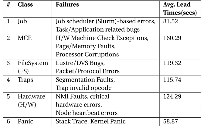
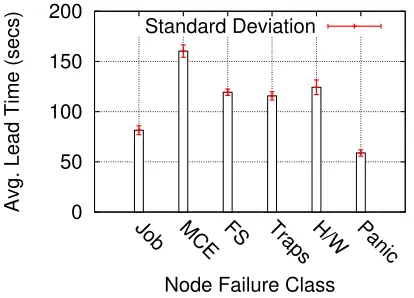
Table 3.8 Node Failure Classes . . . 45

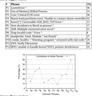
Table 3.9 Unknown Tagged Phrases . . . 48

Table 3.10 Unknown Phrases with and without Node Failures . . . 49

Table 3.11 Desh Comparison . . . 51

Table 3.12 BlueGene/L Log . . . 52

Table 3.13 Desh vs. DeepLog . . . 53

Table 4.1 Log Variations . . . 60

Table 4.2 System Logs . . . 60

Table 4.3 Log Message Processing . . . 61

Table 4.4 Parser Grammar . . . 62

Table 4.5 Multiple Rule Matches . . . 66

Table 4.6 Efficiency Formulae . . . 69

Table 4.7 Speedup . . . 70

Table 4.8 Comparative Analysis of Aarohi . . . 73

Table 4.9 Aarohi Adaptability . . . 74

Table 5.1 HPC System Details . . . 80

Table 5.2 Log Data Details . . . 82

Table 5.3 Fault Breakdown . . . 85

Table 5.4 Root Causes of Failures . . . 92

(10)

(11)

LIST OF FIGURES

Figure 1.1 Lead time to a failure . . . 2

Figure 2.1 Overview of a Cray System . . . 11

Figure 2.2 Correlation with Job Logs . . . 15

Figure 2.3 Time Correlation and Data Integration . . . 16

Figure 2.4 TBP Framework . . . 17

Figure 2.5 TBP Prediction: Topic Modeling for Node Failure Prediction . . . 19

Figure 2.6 Estimate of Node Failures . . . 20

Figure 2.7 Phrase Likelihood . . . 21

Figure 2.8 Mean and Std. Deviation . . . 21

Figure 2.9 Sensitivity of Lead Times . . . 23

Figure 2.10 Recall/Precision/FNR Rates . . . 23

Figure 2.11 Failure Categories . . . 24

Figure 2.12 Lead Times+False Positives . . . 24

Figure 2.13 Phrase Reduction and Order . . . 25

Figure 2.14 False Positive Rate . . . 26

Figure 2.15 TBP Scalability . . . 26

Figure 3.1 Desh with LSTM . . . 35

Figure 3.2 Desh Overview . . . 36

Figure 3.3 LSTM Phases . . . 40

Figure 3.4 Prediction Rates . . . 43

Figure 3.5 FP Rate and FN Rate . . . 43

Figure 3.6 Lead Times+Failure Classes . . . 46

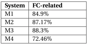
Figure 3.7 Avg. Lead Times of Systems . . . 46

Figure 3.8 Lead Times and FP Rate . . . 47

Figure 3.9 Unknown Phrase Analysis . . . 48

Figure 3.10 Cost Analysis . . . 50

Figure 4.1 Two Phase Failure Prediction . . . 58

Figure 4.2 Overall Design . . . 59

Figure 4.3 Aarohi Design . . . 59

Figure 4.4 Phrase Chains . . . 63

Figure 4.5 ∆Times . . . 64

Figure 4.6 Offline Training to Online Testing . . . 68

Figure 4.7 Phase 1 Efficiency . . . 69

Figure 4.8 W/O Benign Phrases . . . 69

Figure 4.9 With Benign Phrases . . . 69

Figure 4.10 Diverse Platforms . . . 70

Figure 4.11 O3 Optimization . . . 70

Figure 4.12 Token Fraction . . . 71

Figure 4.13 Lead Times to Failures . . . 71

(12)

Figure 4.15 System Prediction Times . . . 72

Figure 4.16 Predictor Placement . . . 76

Figure 5.1 Cray System1 . . . 83

Figure 5.2 Methodology . . . 83

Figure 5.3 Failure Times . . . 84

Figure 5.4 Dominant Cause . . . 84

Figure 5.5 Failure Reasons . . . 84

Figure 5.6 Node Faults . . . 86

Figure 5.7 Heartbeat Faults . . . 86

Figure 5.8 Blade/Cabinet Faults . . . 86

Figure 5.9 Blade Counts . . . 87

Figure 5.10 SEDC Warnings . . . 87

Figure 5.11 Cabinet RPM Faults . . . 87

Figure 5.12 Lead Times . . . 88

Figure 5.13 Lead Times with FP . . . 88

Figure 5.14 External Influence . . . 88

Figure 5.15 Job Failures in S5 . . . 90

Figure 5.16 Job Failures in S2 . . . 90

Figure 5.17 Resource Overallocation . . . 90

Figure 5.18 Root Causes . . . 92

Figure 5.19 Blade Failures . . . 92

Figure 5.20 Temporal Locality . . . 92

Figure 6.1 Improved System Reliability . . . 101

(13)

CHAPTER

1 INTRODUCTION

The past decade has contributed resilience to HPC (High Performance Computing) by proposing

fault tolerant solutions for applications[Vis16; Cha06], reactive recovery approaches such as check-point/restart[Ell12; Tiw14], gaining a better understanding of system logs[Wan17a; Gup15], and comprehending the requirements in terms of performance, resilience and power trade-offs[ El-12a; Nie17]. While computing systems have matured in computing efficiency (operations/second), scale, and evolved architectures, fault manifestation has become complex. Faults are frequent and

are expected to increase with shorter mean time between failures (MTBF) in the next generation

systems[Eln08]. Currently, substantial compute capacity and power is wasted in recovering failed components[ES18]. Failure prediction with defined lead times is the need of the hour to combat such unprecedented faults and failing components.

1.1 Supercomputing Systems

As of November 2018, 28% of the top 100 supercomputers are Cray machines[Top]. In such systems, hardware, software, or application malfunctioning give rise to errors. Errors propagate as faults leading to failures. This work develops a better understanding of failure manifestations in the

current systems and proposes efficient techniques to predict node failures before an unhealthy

(14)

Figure 1.1Lead time to a failure

the following terminologies:

• Phrase: A phrase refers to an event or a log message in any log file obtained from a computing system. Usually, log messages are timestamped, however, they need not necessarily be so.

• Lead Time: The messages or phrases are logged at some timestamp. Lead time is the time difference between the time at which a component became unresponsive and the time at which an impeding failure is flagged proactively at a precursor phrase. This precursor phrase

may or may not be indicative of any error and precedes the terminal messages leading to a

failure. Figure 1.1 illustrates the definition of lead time. Suppose a terminal message indicating a confirmed node failure appears in log message P21 at time T21. If our failure prediction

framework flags this failure after checking phrase P5, the calculated lead time is∆T=(T21 -T5). If it is flagged earlier after checking phrase P4 then the lead time increases to∆T=(T21 - T4), the increase being (T5 - T4). The higher the lead time, the more time remains to take

suitable recovery actions. However, flagging potential failures at much earlier precursor events

may also lead to incorrect predictions (false negatives and false positives), thereby decreasing the accuracy. This makes a lead time sensitivity study essential.

• Prediction Time: Prediction time refers to the time taken to infer whether an incoming se-quence of phrases will lead to a node failure or not. This is also referred to as the inference

time during testing. Prediction time is decoupled from the offline training time.

• Failure: Failures can be in hardware, software or application unless explicitly mentioned. This dissertation focuses on compute node failures.

Supercomputers help conduct intensive scientific simulations and computing. However, their

evolv-ing complex system design and voluminous logs have made data minevolv-ing-based failure diagnosis

non-trivial. In that sense, most technical enhancements become a double-edged sword over a period of time. With applied machine learning-based fault tolerant solutions on the rise, log

(15)

failure prediction solutions for improved resilience. This can avoid expensive checkpoint/restarts saving compute capacity and energy. This dissertation contributes methods for achieving lead times to node failures for predictive localization of anomalies for large-scale computing infrastructures.

1.2 Challenges in Proactive Failure Management

In spite of the fact that a substantial amount of research has been conducted in the context of

anomaly detection[Lan10b; Du17; Sal10], log characterization[Gup15; Gup17; Nie17]and root cause diagnosis[Zhe12; Fu14], failure prediction still requires additional research efforts because of the following concerns:

1. The existing approaches do not evaluate lead times to failures, an indispensable requirement

for proactive actions. Post-mortem diagnosis is not helpful even if accurate. This requires

scalable unsupervised solutions, which can be made to work with noisy unstructured system logs.

2. Online failure prediction necessitates even more stringent timing requirements. Offline

train-ing and event correlation plus validation, even with improved recall and accuracy, do not ensure rapid anomaly prediction. The missing link is quick inference during testing so that the

prediction time is minimal. This then allows a significant fraction of the remaining time before

the component fails to be spent on taking recovery actions such as migration or rescheduling of jobs.

3. Root cause diagnosis considering diverse system conditions across time and space needs

further investigation. Spatial and temporal analysis of different events in an HPC system reveal insights to failure patterns and their characterization. There are many internal as well as

exter-nal conditions and diverse components to consider for resilience actions. Determining what faults and environmental conditions lead to failures in the operational context is challenging.

The next step would be to build frameworks that can propose effective solutions to prevent

failures based on the outcome of such characterizations.

The road blocks to answering the above questions have been that, the past researchers heavily relied on:

• Fatal severity levels to classify anomalies[Fu14]. In older HPC systems, logs were comparatively more structured than Cray systems. Fatal events served as indicators for feature extraction.

• Techniques of Principal/Independent Component Analysis (PCA/ICA)[Lan10a], Support Vec-tor Machines (SVM), Decision trees, Markov chains, and Bayesian models have been applied

for log mining-based anomaly detection. These methods are computationally expensive with

(16)

In recent times, system logs have become more complex and dense because of component scaling

and diverse log sources. New data mining techniques have also been developed such as deep learning[Chi14; Du17]. With the upcoming exascale1_{era, scalable solutions are required for log} analysis unlike prior approaches such as PCA or SVM, which become intractable with scale.

Another concern is the expected short lead time in large-scale computing systems, with MTBFs being reduced originally from hours to a few minutes. It is challenging to obtain short lead times

before a failure happens since the major indicators are prior to the terminal failure messages.

Analysis of a sequence of events over time and space irrespective of log-severity levels is required for accurate failure prediction. A fatal message could be fatal for a component failure during a specific

time frame but benign in another context. Such fine-grained analysis needs a slightly different

approach to failure prediction.

Besides the focus on time sensitivity, tracking the location of failure is also important so that

recovery actions can be taken assuming system logs are vendor controlled and cannot be modified

as per our convenience. Moreover, anomaly injection[Yu16], source code reference[Xu10], and binary instrumentation have been applied in several anomaly detection works in distributed systems

but are inappropriate for HPC systems. Supercomputing systems produce lower-level Linux-style

logs, which are not application centric. Instead, they consist of OS-level timestamped events. Low level hardware and software malfunctioning is a concern in addition to application bugs. Hence,

HPC systems require extensive data correlation and integration to understand the intricacies of anomalies at the lower systems level.

It is time we investigate failure prediction in the light of the above concerns to improve the

reliability of the current and next generation computing systems.

1.3 Problem Statement

This dissertation aims to answer the following questions:

“Can we predict that a node is about to fail before it stops responding? If so, how much ahead of

time can this prediction be done and with what level of accuracy?"

It should be noted that we want to use the nodes exhaustively before any one node fails, i.e.,

we do not want to flag an impending failure too early when the node is functioning without any

anomalies. In that sense,just enoughlead time is essential in the context of finishing any feasible proactive action (e.g., live migration within 30 seconds). Otherwise, if a failure was flagged late, just

(17)

before the failure manifests (e.g., 10 seconds), proactive resilience may no longer be feasible, i.e., the

node’s state can no longer be migrated or saved by any means before the failure occurs. However, it may or may not be always feasible to procuresufficientlead times to failures, i.e., flag a failure in a

timely manner. How much lead time can be achieved depends on how the nodes fail in different

systems over different time frames. How similar or dissimilar the sequence of phrases are in the logs leading to a failure versus healthy logs influences the prediction accuracy. In this context, we

wish to achieve sufficient lead time with an acceptable false positive rate.Acceptableindicates the

fact that the majority of the failures can be predicted with minor prediction inaccuracies. We do not put a singular lower bound on the lead time, as different failures pertain to different patterns.

Depending on an immanent failure, diverse lead times may be obtained with a limit on the false

positive rate. This dissertation addresses this problem of lead time estimation for failing nodes in production systems.

1.4 Hypothesis

We have identified the prerequisites to enable practical failure management in computing systems

(Section 1.2), i.e., scalable semi-supervised log mining solutions with defined lead times. The

con-jecture is that feature extraction from and dimensionality reduction on contemporary system logs is difficult. But, at the same time, sufficient numerical and textual information is contained in these

logs to take timely precautionary actions. We may not be able to avoid inaccurate predictions at all

times but lowering the false positives and false negatives will contribute to making systems more resilient and to saving compute resources. The challenge is to gain clarity in understanding how

faults propagate in the system causing component failures and finding the middle ground where

failures can be flagged with sufficient lead time, yet an acceptable false positive rate. We state the following hypothesis for developing failure prediction techniques:

“The majority of node failures in HPC systems can be predicted via machine learning thereby

identify-ing the precise node location and with sufficient lead time to engage in proactive actions for fault

mitigation".

1.5 Thesis Contributions

This dissertation contributes a characterization of achievable lead times to node failures in HPC systems by exploring contemporary machine learning/deep learning techniques. This can aid in assessing the potential for proactive failure management through a time sensitive study involving

(18)

following specific contributions:

1. Chapter 2 describes TBP (Time-Based Phrase), a topic modeling-based approach for

produc-ing lead times to node failures. This scheme demonstrates the requirement of continuous time probabilistic likelihood estimation to decipher emerging event phrases over diverse time

intervals. The job logs and system logs are correlated before training. Trained node failure

chains are formulated with the help of terminal messages and confirmed in consultation with the system administrators of the facility. TBP checks for impending failures in the test data

by comparing with the trained failure chains. Depending on the phrases that form a failure

chain, lead time is calculated from the terminal message to the specific phrase where a failure is flagged. TBP achieves as high as 86% recall and 16.66% false negative rate. With 2 minutes

average lead time, the false positive rate does not exceed 23%. Additionally, this study shows

that 15 to 20% of the nodes fail due to hardware errors, machine check exceptions (MCEs). and kernel panics, while bit errors and application-caused errors are minor contributors.

2. Chapter 3 proposes Deep Learning for System Health (Desh), a deep learning-based method

to predict lead times to node failures. Desh uses long short-term memory (LSTM) to train

events to form failure chains, re-train chains of events augmented with time differences to learn expected lead times, and eventually predict lead times during testing. Desh obtains at

least 83.6% accuracy and 85.7% F1 score along with as high as 87.5% recall rates. It obtains on average 2 minutes lead times with no more than 25% false positives. Desh illustrates the

importance of examining a timed sequence of events for anomaly prediction over a single log

message, since a message may be fatal in one but benign in another context. Thus, log-severity levels are inaccurate indicators for failure prediction. Furthermore, this work finds that lead

times of similar failure classes are comparable with insignificant variability while the lead

times tend to vary over diverse classes of a specific system.

3. Chapter 4 contributes a fast node failure predictor calledAarohi. It is designed to be generic and scalable to effectively infer failures online through context free grammar-based rapid

event analysis. Aarohi obtains more than 3 minutes effective lead times to failures with an

average of 0.31 msecs prediction time for a chain length of 18. The overall improvement in inference speedup obtained w.r.t. the existing state-of-the-art is over a factor of 27.4x. This

compiler-based approach depicts the merits of leveraging an efficient parser suitable for

real-time streaming logs.

4. Chapter 5 explores holistic root cause diagnosis of node failures using a measurement-driven approach on contemporary system logs that can help vendors and system administrators

support exascale resilience. Empirical evidence suggests that environmental influence is not

(19)

faults trigger failures, the underlying root cause often lies in the application malfunctioning.

Lead time enhancements are feasible for nodes showing fail slow characteristics. This study excavates such helpful insights, which can facilitate better failure handling in production

systems.

1.6 Dissertation Organization

This dissertation is organized as follows. Chapter 2 presents a node failure prediction framework

using topic modeling, an NLP-based approach for supercomputing systems. Chapter 3 contributes a deep learning-based mechanism to predict lead times to potential node failures in HPC systems.

Chapter 4 proposes a compiler-based failure predictor to infer imminent failures with enhanced

speedup. Chapter 5 describes root cause analysis of node failures adopting a holistic approach considering external and internal event correlations. Chapter 6 discusses the deployment efforts of

the developed failure prediction solutions and concludes with potential future work in the context

(20)

CHAPTER

2 PREDICTING WHICH NODE WILL FAIL

WHEN ON SUPERCOMPUTERS?

2.1 Introduction

Significant efforts have been made to improve the resilience of HPC systems in recent times. Existing health check monitors and techniques such as root cause diagnosis and failure detection use diverse

log sources to combat failures. However, they still fall short of strong means to handle node failures

proactivelyin complex, large scale computing systems. First, supercomputing systems are constantly changing due to novel architectures, design, upgraded applications and logging mechanisms. Prior

techniques of automated fault diagnosis do not suffice for the evolving changes[Bra15].

Second, existing HPC infrastructures with their increasing component count required for ex-ascale (≈106_{nodes) make accurate fault prediction hard. Aborted jobs due to node failures inflict} significant energy costs[Mar15b]. More than 20% of the compute capacity is wasted in failures and recovery, as reported by DARPA[Eln08]. With increasing number of nodes, the mean time between failures (MTBF) reduces for a node, making fault identification and resolution even more difficult.

Increasing complexity in emerging next generation systems obviates the need for adaptive fault aware solutions to address this critical reliability challenge.

To address this challenge, we present a fault-tolerant solution to pin-point potential node failures

(21)

techniques such as checkpoint/restart and redundancy/replication incur additional costs[Ell12]. Our methodology to identifywhich nodesare likely to fail (location information) prior to actual fail-stop behavior can reduce the overhead of failure recovery.

HPC resilience has been investigated extensively. Prior work has characterized system logs in

the context of fault detection and prediction. While most work focused on anomaly detection in BlueGene systems[Fu14; Yu12; Ber14; Lan10a], time sensitive failure prediction in the context of Cray supercomputers with their lower-level Linux-style raw logs has not been researched exhaustively

yet. As of November 2017, 29% of the top 100 and 40% of the top 10 supercomputers (e.g., Titan, Cori, Trinity)[Nov]were Cray machines. It is important to investigate Cray machines more closely to explore techniques that increase reliability. This paper discusses the inherent challenges of Cray

systems and proposes a mechanism to predict node failures.

Motivation

From log data analysis to root cause diagnosis across various levels (hardware, system, application)

researchers have studied failure manifestations in HPC systems and devised ways to improve recall

rates[Gai13]. In spite of such a large body of work on resilience, further investigation is required for the following reasons:

1. Existing work performs prediction and diagnosis without sufficient emphasis on lead time requirements. Pin-pointing which nodes will fail well ahead in time to proactively counter

performance disruptions still remains a challenge. Optimal learning window interval selection

and determining appropriate lead times are important considerations for successful prediction of node failures.

2. Most prior studies[Yu12; Zhe12; FX07]use the same training data for future predictions over a long time frame. As hinted by Gainaru et al.[Gai13], correlations determined off-line are dynamically adapted, having limitations when using a short training set for a long

future time window. This limitation makes prediction impractical on real production systems.

Investigations of dynamic learning and scalable online prediction techniques are required to improve prediction efficiency.

3. There exist unpredictable failures[Gai13], and we need to understand HPC Linux/Cray systems in finer detail to determine where correlation extraction from system logs is hard.

4. Validation of predicted faults is commonly done through comparison with event logs

(some-times with identical training and testing data) or by consulting system administrators. Relying on manual human expertise or system administrator’s knowledge is difficult at times. It is

important to explore if alternate validation schemes could be formulated for good prediction

(22)

We focus on the 1st and 3rd aspects in this paper. This work is a step forward to address the above

mentioned hurdles in locating node failures in HPC systems.

Contributions

This paper shows a novel way to extract failure messages indicative of compute node failures for Cray systems. First, we provide an analysis of Cray system logs and job logs and show how failure

prediction in such systems poses additional challenges compared to systems such as BlueGene. Second, we discuss what node failure exactly means in the context of Cray systems, what traits

govern normal shutdowns and abnormal reboots and how we can avoid trivial pitfalls in node failure

detection. We provide frequency estimates of compute and service node failures highlighting their potential consequences on systems and user applications.

Finally, we propose a novel prediction scheme, TBP (time-based phrase), to extract relevant

log messages indicative of node failures from noisy data. This scheme relies on phrase likelihood estimation considering continuous time-series data to elicit out useful messages. These events help

forecast future failures with lead times ranging from 20 secs to 2 minutes.

2.2 Background

Let us provide a brief overview of the system logs studied highlighting the main components of

such logs used for analysis. Table 2.1 summarizes the system and job logs collected from three contemporary systems, namely: SC1, SC2 and SC3. The timespan of SC1 and SC2 logs exceeds a

year, SC3 logs cover less than a year. Size refers to the log data size and scale indicates the cluster

size in terms of the number of compute and service nodes. Most of the systems belong to the Cray XC series that have been widely deployed and typically run more than 1,400,000 jobs/year.

Table 2.1System Details

System Duration Size Scale Type

SC1 14 months 573GB 5600 nodes Cray XC30 SC2 18 months 450GB 6400 nodes Cray XE6 SC3 8 months 39GB 2100 nodes Cray XC40

Cray System Architecture

Figure 2.1 shows a high-level overview of a Cray system. A job scheduler distributes user jobs on the

allocated compute nodes. Production jobs are executed on the compute nodes and external clients access the cluster through the login nodes. The parallel file system (e.g.Lustre) and a network server

(23)

nodes and compute nodes. TheSystemManagementWorkstation (SMW) administers and logs various cluster components and monitors resource usage. TheServiceDatabase Node (SDB) stores information of all the service nodes. The boot node manages the shared file system with service

nodes. Login, boot and SDB are some of the service nodes of the system in addition to syslog, I/O and networking nodes. TheApplicationLevelPlacementScheduler (ALPS) processes such as

aprun

,

apbridge

,

apshed

,

apinit

etc. are responsible for user application submission and monitoring and run on both service and compute nodes.

Figure 2.1Overview of a Cray System

Table 2.2 indicates the major log sources. From these archived logs, we consulted p0-directories

that contain comprehensive logs of the entire system with information pertaining to the internals of compute nodes including system and environment data. We use the acronymidto refer to

node or job identifiers. The files (console/message) in these directories contain timestamped event logs including node ids (cX-cYcCsSnN) per line. We track the node ids per log line (event) while correlating and integrating data. Logs can contain extended node ids (nids), which can be converted

to the cX-cYcCsSnN format to identify a node’s location such as blade(S), chassis(C), cabinet(XY)

and the node (N). Additional references to boot messages and job logs aid the prediction scheme since they provide the status of nodes and jobs over time.

Table 2.2Data Details

Source Content

p0 directory Internals of compute nodes Boot Manager Boot node messages Log System

rsyslog

messages

Power/State Logs Component power and state information Event Messages Event router records

(24)

We found that noisy information pertaining to power management, SMW, the log system,

net-work interconnect logs, events, and the state manager, are not very useful for node failures and, hence, have not been considered. These lower-level logs did not reveal significant textual indicators

related to node failures. Manuals/system administrators help to understand logs, but even then post-mortem analysis for unsupervised information extraction remains non-trivial from such data.

Technical Challenges

The challenges of data diversity, system complexity, and overwhelming logging volume have been

in-vestigated in the context of failure detection[Lan10b; Zhe12]. Furthermore, Cray systems specifically have the following additional challenges:

1. BlueGene systems have Node Card, Service Card, Link Card and Clock Card components, each

of which provide current, voltage, temperature data etc. In Crays, failure needs to be discovered

by integrating a distributed set of events in space and time, coming from different system components, some of which are replicated. Feature identification even before dimensionality

reduction is hard.

2. Binary or numeric values (normalized or mapped) of features as considered in prior work[Yu11; Yu12]do not suffice. Simple absence or presence of an event is not enough. Which event, when did it happen, is it related to the node under consideration and similar factors are also

of importance here.

3. RAS logs in BlueGene systems contain fatal and warning flags indicating the severity levels

with the log messages[Zhe11; Zhe09; Hac09]aiding researchers to segregate between failures and benign events. Critical and warning flags are present in Crays as well pertaining to certain

components such as

netwatch

,

pcimon

etc. However, direct classification of log messages

based on occasionally appearing flags is ineffective[Zhe09]for long-term time sensitive data since several non-critical messages could be a better indicator of failures over time. Besides,

seemingly benign events in one context may lead to fatal events in another, which means

BlueGene logs may result in shorter lead times. Hence, we consider phrases irrespective of flags/severity-levels.

4. There exists unsteadiness in timestamps between service nodes, job schedulers (Slurm/Torque) and compute nodes making time-based correlation non-trivial. Time-series analysis handles

(25)

Node Failure

The boot log reveals several clustered node failures caused by problems ranging from

communica-tion failures, network-interconnect and applicacommunica-tion-based errors, resource-contencommunica-tion, file system or hardware errors. Further study revealed certain patterns in the context of node failures. If nodes

shut down in bulk (multiple blades) within a few seconds, the root cause tends to be maintenance.

Such shutdowns often are massive (e.g., 98 or 126 nodes going down at once). But even in case of single compute node failures, the culprit could be either external or internal events (see Table 2.3).

Table 2.3Node Shutdown Events

Internal Failures External Failures Normal Shutdowns

Application Bugs Blade or Cabinet Controller Issues Massive shutdown Node System Bugs File system or Network Server Issues Maintenance Reboots Node Hardware Issues Router or other Hardware Issues Periodic Node Reboots

• Internal Events are compute node specific events either caused by applications running on that node or hardware/software problems related to memory, kernel etc. pertaining to that node.

• External Events are events that occur outside a specific compute node such as Lustre

server-related errors, a Link Control Block (LCB) failure, or a network interconnect failure causing multiple chassis to shutdown. Cabinet- or blade-controller problems can also manifest as

massive node failures.

Node Failure Definition:Not every node unavailability indicates an anomaly. Power outages,

maintenance and deliberate shutdowns have been eliminated in our study. Cases related to the internal and external events (discussed above) are considered as node failures since they manifest

as anomalies.

Periodic service reboots are common in Cray nodes. Nodes are rebooted several times before they

come up as part of regular maintenance. Such spurious cases are not counted as node failures since

these are not caused by any faults in the system. Counts of node failures do not consider unique nodes since a specific node can fail multiple times at different timestamps. Unresponsive nodes, stress

testing, and changing power cooling conditions manifest in log messages and have been considered in our study; a failed heartbeat indicates failure with unknown root cause (network/OS/hardware failures resulting in lost connection) and are indistinguishable from anomalous node failures in

terms of manifestation. We have timestamped logs, and based on the time and scale of shutdowns,

we segregate failures. In many instances, service node failures impact compute node failures (see Sec. 2.5).

(26)

Table 2.4Examples of Node Failures

bit flips caused failure hardware caused failure app. caused failure

4.25.30 pm 8.44.12 pm 2:44:49 am

LCB on and Ready Hardware Overflow Error Matlab invoked oom killer

4.30.33 pm 8.46.09 pm 2:54:14 am

Micropacket CRC Error Messages Lnet errors Recvd down event Out of memory: Kill process

4.35.29 pm 8.47.45 pm 2:58:14 am

Network chip failed due to too many soft errors

Lustre Errors Binary changed Killed process

4.36.42 pm 8.48.06 pm 2:59:40 am

Aries LCB operating badly, will be shutdown

Bad RX packet error Kernel panic not syncing:

4.37.31 pm 8.52.37 pm 3:00:00 am

Failed LCB components Out of memory/Killed processes page_fault+0x1f/0x30

4.37.39 pm 8.55.13 pm 3:00:03 am

2 nodes unavailable Node unavailable Node unavailable Failed within12 min. Failed within11 min. Failed within16 min.

chains of time-based events, which eventually led to a failed node. The actual cause and the location

of a root cause may not be indicated by our prediction methodology. E.g., in Table 2.4 column 1 (bit

flips), after repeated soft errors a Link Control Block (LCB) went down. The cause of

CRC error

messages

may range from hardware (link/NIC) problems to silent data corruption, but this cause is of no concern for our analysis.

Illustrative Examples:Table 2.4 shows three cases of node failures. The first column shows a

case of a failure caused by soft errors (bit flips) detected by the LCB. Due to too many errors the LCB

went down after which 2 nodes of a blade went down within 12 minutes. The second column shows

the case of a hardware error caused by the network interconnect. This triggered Lnet and Lustre errors followed by memory problems, and the node went down within 11 minutes. The third column

shows an application (Matlab) failure caused by excessive memory allocation. This killed several tasks, followed by a kernel panic, failing this specific node. In these cases, if prediction happens a

few minutes before the actual shutdown, some proactive measures can be taken.

2.3 Predictor Design

We model our method after unstructured phrase mining approaches applied in the context of

Natural Language Processing (NLP) research. Our study shows that Topics over Time (TOT)[WM06] (an LDA-style[Ble03]unsupervised topic model) based learning can help pin-point faulty nodes. Identifying rare compute node failures by relating job ids, which arere-runseveral times on the

(27)

Figure 2.2Correlation with Job Logs

Job Logs

Figure 2.2 demonstrates how jobs scheduled on allocated nodes are identified in the ALPS logs

inside the p0-directories. The job server such as Torque provides information about job id, the allocated nodes for that job and the status. These can be referenced in the ALPS logs through a

mapping conversion. The job ids map to batch ids. The node naming convention is derived from

the boot logs, which provide the required id for system logs, and the job information is referenced using

res

,

app

and

pagg

like tags added by ALPS. The timestamp is considered for correlation

by checking the amount of slack in logs from different sources (job, server/compute node). If it is within a given threshold (we observed 15 seconds to be appropriate), it is considered. This did not cause any correlation errors since the ids were matched correctly over time. In our experience,

missing data in log archives and MOM (machine-oriented miniserver) node failures (see Figure 5.1) affecting job data complicates this correlation across the available logs. This arises due to stopped

daemons/logging, with or without upgrades. Nonetheless, this presents a legitimate way to track the behavior of jobs running on nodes. However, upgrades and changes in job schedulers (ALPS-Torque, ALPS-Slurm) can create inconsistencies in the available data. But this does not hamper the

prediction mechanism since the correlation has been confirmed by prior offline manual validation

with system administrators, and only complete and consistent data is used for evaluation.

Data Integration

After successful correlation, a text document with timestamps, node ids and filtered log messages is

formed to generate a viable input for the statistical probabilistic model (Figure 2.3). We do not use

any particular environmental data, such asSystemEnvironmentDataCollection (SEDC) logs, since such information predominantly does not aid in phrase extraction. Temperature and voltage values

may indicate an anomaly but our work intends to discover salient phrases providing symptoms of

(28)

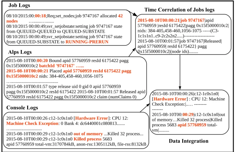
Figure 2.3Time Correlation and Data Integration

Phrase Likelihood Estimation

One primary tendency observed in the available logs is the recurrence of failure messages over

time and changing patterns that continuously evolve over time. A phrase is defined as an event log

message corresponding to a specific node at a certain timestamp. This trend of time-based evolution prompted us to leverage a well known machine learning technique called Latent Dirichlit Allocation

(LDA)[Ble03], a probabilistic model on discrete data. One important factor for log analysis targeting prediction is time. Hence, continuous time series-based evolution is required to extract patterns

from the integrated document. To address this, we utilize theTopicsoverTime (TOT)[WM06] algorithm to identify the top

N

topics (i.e., phrases or log messages) over a period of time and track how the topics change over time. TOT employs Gibbs Sampling and is useful for dynamic

co-occurrence of patterns when an upsurge and downfall of phrases exists over time. Since TOT

models time in conjunction with frequency of phrases, which is analogous to the case in temporal logs, TOT is a good choice for our study in contrast to other existing competitive approaches such

as[Nak11; Zhe09; Hac09; Zhe10; Yu16].

On similar grounds, discrete-timeDynamicTopicModeling (dDTM)[BL06]is inappropriate since there is a significant variation in occurrence of events (at the granularity of milliseconds)

so that several chunks of logs cannot be clustered under a single time instance. Coarse-level time

(29)

Figure 2.4TBP Framework

assigned a topic. Multiple phrases can be assigned the same topic (see Table 2.5). We have finite

number of topics for an integrated document. During the training phase, TOT learns top

N

topics

referring to phrases. TBP forms sequences of phrases that correspond to failures in the past referring to the data. We use them to forecast future failures when those phrases reappear in the test data.

Once we know the significant phrases, we denormalize their timestamps and refer to the nodes associated with them to identify nodes subject to future failures. We name our prediction mechanism

“time-based phrases” (TBP).

Table 2.5Topic Assignment

# Event Phrase Topic

1 Lnet: waiting for hardware.. Lnet

2 Lnet: Quiesce start.. Lnet

3 Debug NMI detected NMI

4 DVS: uwrite2: returning error DVSBug 5 Kernel panic/not syncing/Fatal Machine check Panic

6 MCE threshold of fff.. MCE

2.4 TBP Framework

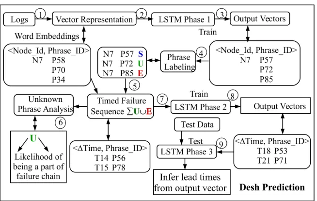
Figure 2.4 shows the work-flow diagram of our approach. After job and system data correlation and

formation of an integrated document, we obtain the top ranked phrases over time and determine the nodes corresponding to them (Box A). Then, based on the time series, TBP obtains a chain of

messages leading to the node failures. We use them on test data to compute recall rates and lead

(30)

Time Correlation

Figure 2.3 illustrates the idea of time correlation. The job log indicates that at

00:18

a job with id

9747167

is allocated 42 nodes. This job is correlated with its corresponding ALPS message

apid

57760959

,

resId 6175422

,

pagg 0x15f5000010c2

logged at

00:20

, just 2 seconds later. Since 2 seconds are within the threshold (15 seconds), these become correlated. Simultaneously, we obtain

the ids of nodes allocated to this job by converting from

nid

(extended node id) to the

cX-cYcCsSnN

format. These node ids and job ids can be time correlated to the rest of the logs (e.g., console logs)

in a similar fashion as shown in Figure 2.3.

TBP Learning

TBP uses TOT to learn the failure chains from the training data. Topic assignment assigns a relevant topic to every phrase pertaining to that topic as shown in Table 2.5. We have used more than 100

topics in our training data. Multiple phrases can be assigned the same topic if the content of that

phrase is not anomalous or if they have similar system event context (e.g., 1 & 2). A distinct phrase can also be assigned a topic if it indicates a unique event (e.g., 3 & 5). TOT chooses top

N

topics (i.e.,

phrases) as shown in Figure 2.5.

Let us explain how TOT picks the top

N

topics. The basic idea is that phrases chosen are localized in time. As the distribution of phrases changes over a continuous time frame, top phrases evolve

since the phrase co-occurrence changes[WM06]. The 8 topics (firmware bug, ec_node_info, Lustre, DVS, LNet, hwerr, apic_timer_irqs and krsip) shown in the illustration Figure 2.5 (box 1) pertain to phrases containing that topic. TBP uses the top picked phrases over time to formulate the failure

chains. Topic-based training helps to extract only the significant phrases relevant to failures (boxes 2+3).

We varied the value of

N

in different data sets to ensure that we are not missing relevant phrases.

In our experiments,

N

ranges from 50 to 80 based on the amount of data considered. We manually inspected the output of TOT while choosing a subset of

N

considering time and space constraints.

To clarify,

N

has been varied but it is impractical and inefficient to inspect too large of an

N

value.

TBP has chosen a smaller subset (smaller

N

) at times to effectively collect indicative phrases.

Node Failure Prediction

How does TBP predict node failures based on top

N

? Figure 2.5 illustrates the key idea of prediction.

T denotes timestamps, N stands for node ids, and P for phrase ids (for brevity we omitted job ids

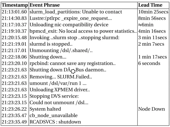
in the figure). The integrated document (Figure 2.3) is trained using TOT. We know the terminal node shutdown messages from sysadmins (e.g.,

System halted, cb_node_unavailable

, see

Table 2.10, last 10 phrases). TBP forms failure chains linking phrases among the top

N

with

(31)

Figure 2.5TBP Prediction: Topic Modeling for Node Failure Prediction

failure chains as shown by C1, C2 and C3. During testing, no top phrases are generated. TBP compares

the incoming phrases with those in the failure chains. If chains with at least 50% similarity in log messages are formed, the corresponding node is likely to fail in the future. E.g.,

p98

and

p36

are

rejected since these were not seen in the training data, and the remaining phrases match with C1 till

P78

. In the test data, before

N12

fails, we compare and predict it to be a potential failure. From

N12

(i.e.

cX-cYcCsSnN

) we can easily derive the node’s exact location in the blade(

S

), chassis(

C

) and the

cabinet(

XY

) to potentially trigger proactive resilience actions before it fails at a future timestamp (

T44

). About 1 month’s data is used for training. The test data is comprised of a moving time window

of 3 days to 1 week for generating better lead times.

2.5 Experimental Evaluation

We have implemented a prototype of the TBP predictor using the factorie[McC09]library and python. We use TBP on 3 datasets from SC1, SC2 and SC3 supercomputers (Table 2.1) for evaluation.

TBP achieves as high as 86% recall rates with acceptable lead times in predictive fault localization of nodes. Our time-series based phrase mining approach works for any HPC system with “text-based”

logs. The evaluation focuses on Cray logs, but the approach is generic to modern HPC systems (see

discussion at the end of this section).

Average Node Failure Estimate

Figure 2.6 shows an estimate of service and compute node failures over 4 months of the data in

(32)

0 10 20 30 40 50 60 70 80 90

SC1 SC2 SC3

#Node Failures

Systems Failures/Mon

Std. Dev

Service Compute

Figure 2.6Estimate of Node Failures

number of service node failures. Our observation indicates that both service and compute node

failures are randomly distributed over time. Hence, this could be misleading in terms of estimating

failure rates over longer periods of time. E.g., over a period of 3 weeks, SC3 encountered 10 service node failures, but the subsequent time periods of 9 days and 2 weeks had 0 and 1 service node

failures, respectively. There exists sufficient variability of failures over time across the three systems.

This explains the standard deviation of the frequency ranging from±6 to±11. Nonetheless, this gives us an idea of the number of failures encountered in such systems.

One might argue, if node failure events are relatively rare compared to the overall scale of

anomalies in the system, why do we need to predict them and take proactive actions? In this regard, we have summarized two main takeaways:

1. The number of compute node failures increases dramatically with an increase in service node

failures. On multiple occasions, time periods with high service node failures have affected

a large number of compute nodes around the same time due to external failures. We did not investigate further the exact root cause of each failed compute node, but in addition

to maintenance related shutdowns, controlled service node failures can definitely prevent

compute node failures, which benefits jobs of users running on them.

2. Rescheduling a job after a node failure delays the overall job execution time and utilizes additional resources. A single job, on average, is generally allocated to many compute nodes

(up to tens of thousands for peta-/exascale capability jobs). If blades fail repeatedly, the effect is logged as independent job failures, which are rescheduled. Past work has observed that a significant fraction of applications fail due to system problems apart from user-related

(33)

Table 2.6Phrase Extraction

# Phrases Probability

1 Ensure file system is mounted on the server and then restart DVS

0.0214

2 LNET: waiting for hardware quiesce flag to clear

0.0145

3 nscd: nss_ldap: failed to bind to LDAP server

0.0167

4 LustreError: *:*:...unable to mount 0.0298 5 startproc: nss_ldap: failed to

bind/reconnecting to LDAP server

0.0302

6 Error: No data from cname 0.0178 7 Lustre: skipped * previous similar

mes-sages

0.0119

8 Lustre:*:*:vvp_io.c:*: vvp_io_fault_start 0.0176 9 reconnected to LDAP server 0.0247 10 Lnet: * Dropping PUT from * .... 0.0218

Phrase Distribution

Table 2.6 shows a sample snippet of 10 phrases over a time window of 2 weeks with their probability

distributions depicting a compute node failure case caused by Lustre server-based errors. The

table shows that Lustre, Lnet and filesystem-related messages are produced by TBP with higher probability than other system messages. These phrases are related to filesystem problems impacting

the node. We do not care about individual probabilities as long as the top

n

phrases are of interest

in the context of node failures.

0 0.05 0.1 0.15 0.2 0.25 0.3 0.35

0 p1 p2 p3 p4 p5 p6 p7 p8 p9 p10 p11 p12 p13 p14 p15

Probability

Phrases from Logs 6 hours

12 hours 21 days8 days

Figure 2.7Phrase Likelihood

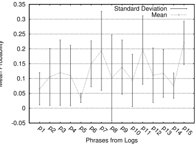
-0.05 0 0.05 0.1 0.15 0.2 0.25 0.3 0.35

p1 p2 p3 p4 p5 p6 p7 p8 p9 p10 p11 p12 p13 p14 p15

Mean Probability

Phrases from Logs Standard Deviation

Mean

(34)

Table 2.7Recurring Phrases

No. Phrases

P1 crms_wait_for_linux_boot: nodelist: * P2 Lnet: Quiesce start: hardware quiesce P3 Wait4Boot: JUMP:KernelStart * P4 krsip:RSIP server * not responding P5 startproc: nss_ldap: failed to bind P6 checking on pid *

P7 LustreError: *:*:...can’t find the device name

P8 GNII_SMSG_SEND+* P9 No ...bios_settings file found P10 Lnet: Added LNI *

P11 DVS: file_node_down: removing * P12 Lustre: skipped * previous similar

mes-sages

P13 Lnet: skipped

P14 <node_health:*> RESID* xtnhc FAIL-URES

P15 Bad RX packet error

Table 2.8Evaluation Metrics

Metric Formula & Implication

Recall TP/(TP+FN) # Node failures, TBP

correctlypredicted

Precision TP/(TP+FP) # Total node failures, TBP predicted

FP Rate FP/(FP+TN) # False Positive Rate True Positive

(TP)

# Actual node failures, TBP suc-cessfully predicted

True Negative (TN)

# Nodes actually didn’t fail, TBP did not predict as failure

False Positive (FP)

# Nodes actually didn’t fail, TBP predicted as failure

False Negative (FN)

# Actual node failures, TBP failed to predict

Observation 1:Significant phrase variation exists over short time intervals. HPC logs indicate event changes at a high frequency, which calls for continuous-time statistical models that can handle this

variability prior to identifying phrase relevance for node resilience.

Figure 2.7 and Table 2.7 illustrate the variation in probability of occurrence for the same 15 phrases

over four continuous time intervals (6 hours, 12 hours, 8 days and 21 days) for SC3 data. The 4 disjoint time frames have been selected from over 3 months of data and illustrate the lack of a

uni-form distribution. Table 2.7 depicts frequently occurring system log messages pertaining to Lustre,

Lnet etc. Figure 2.7 shows the fluctuations of phrase probabilities over different time intervals. We provide a quantitative analysis of such variations to signify the lack of discernible features. Pattern

extraction with such non-uniform distribution of unstructured log messages but without clearly

flagged errors is hard.

Figure 2.8 quantifies this variance through mean (curve) and standard deviation (indicated by the

error bars). The standard deviation for most phrases is high (e.g., for

p7

,

p8

and

p11

), except for

p5

.

As an example, message

p7

is emitted by Lustre for an unmounted device with a higher probability distribution in the 2nd (12 hours) and 4th (21 days) time intervals, but the device was mounted and

the message occurred less in the 1st (6 hours) and 3rd (8 days) time intervals. Similarly,

p11

indicates

a Data Virtualization Service (DVS) server failure, which is removed from the available mountpoint list. The failover event occurred with a different magnitude over the intervals for multiple nodes.

(35)

0 20 40 60 80 100 120 140 160

0 5 10 15 20 25

Lead Time in Seconds

Node Failures 20% Reduction

30% Reduction

Base Lead Time

Figure 2.9Sensitivity of Lead Times

0 20 40 60 80 100 120

SC1 SC2 SC3

Percentage (%)

Systems Recall

Precision False Negative

Figure 2.10Recall/Precision/FNR Rates

was successful after a few attempts in those time intervals. Discrete-time statistical methods[Hac09] are ineffective under such variability.

Prediction and Lead Time Analysis

Phrases detected during the learning phase of around 4 weeks help in node failure prediction on

new test data. TBP checks the test data for phrase similarity relative to the training data (Figure 2.5). If similar, we obtain the node ids corresponding to those phrases and compute recall rates. N-fold

cross validation is less effective for time-series data. Our train and test data split respects temporal

event ordering, (lower-order time-series training, higher-order testing). TBP uses the standard eval-uation metrics of Recall and Precision to estimate prediction efficacy. Table 2.8 enumerates their

formulae and the implications in the context of node failure prediction. The recall rate is defined

as the fraction of node failures that are correctly predicted by TBP, and precision rate as the total fraction of node failures predicted by TBP (need not be correct). The FP rate is the false alarm rate,

the ratio of actual failures missed by TBP. Validation is performed by manually checking the logs

with the timestamps of actual failures. In the test phase, we consider 3 days’ to 1 week’s data, and compare the phrases with the obtained trained data. We re-train (4 weeks data) and move the test

data time interval with shifts of 1 week to predict impeding failures and procure lead times. The base

lead times in Figure 2.9 considering the trained failure chains are in the range of 20 to 60 seconds without any phrase reduction. We have optimized TBP’s lead time sensitivity further through phrase

pruning.

Observation 2:TBP achieves high recall and precision with a modest number of false negatives and as high as 1 minute base lead time.

(36)

0 5 10 15 20 25

Kernel MCE FS SWERR Soft App HWERR

Percentage (%)

Failure Types Failures

Figure 2.11Failure Categories

0 5 10 15 20 25 30 35 40

0 1 2 3 4 5

Percentage

Lead Times (mins) False Postive Rate

Figure 2.12Lead Times+False Positives

Table 2.9Major Failure Categories

# Failure Type Class

1 Trap invalid opcode/Segfaults, File System Bugs Software 2 cb_hw_error: failed_component, Firmware Bugs, NMI Faults Hardware 3 [hwerr]: Machine Check Exception (MCEs), Memory faults Hardware 4 RCU CPU Stalls/Hangs, Kernel Panic/Fatal Exception, Stack Trace Software 5 Bit/Packet Errors (dla_overflow error. Msg protocol error) Soft Errors 6 Machine Check Events (Node heartbeat faults) Hardware

7 Job Server/Task related errors Application

up to 99%, which indicates a low rate of false positives. This indicates that the trained failure chains were indeed indicative of node failures. The recall rates are 86% or lower. TBP aims not to miss

actual node failures irrespective of the causes and correlations between them. Even if correlated

failures are removed, precision and recall exceed 80%. Across all the 3 systems the false negative rate is as high as 16.66%. This is partly because of the new phrases seen while testing and partly

due to the corner cases where phrase extraction is difficult. SC2 has a relatively low false negative

rate since failure events learned during training were mostly seen during testing with similar failure types (e.g., networking problems). Figure 2.10 rates correspond to the base lead time without any

phrase pruning.

Observation 3:Hardware errors, MCEs and kernel panics often cause node failures. Minor causes are failed components in the network interconnect, bit errors, filesystem caused errors and application based errors.

Figure 2.11 shows the proportion of different types of failures observed in the data, namely Kernel

(37)

Figure 2.13Phrase Reduction and Order

(bit/packet/protocol related soft errors), App (application errors), and HWERR (hardware node heartbeat faults), respectively. Table 2.9 lists the major classes of anomalies manifesting in node disruption in such systems. While 15 to 20% of the nodes fail due to H/W errors, MCEs and kernel panics, bit errors and application caused errors are minor contributors. Our observations conform

to failures reported by Gupta et al.[Gup17].

We predict node failures on average a minute in advance; this is an improvement over scenarios where nodes fail within 20-30 seconds of the occurrence of the first reported event that can be linked

to a later failure by system administrators. However, certain failures such as NMI faults cause instant failures without a chance to communicate anymore. It is impossible to take proactive actions in

those cases. Moreover, many indicative messages occur just prior to the failure.

Lead Time Improvements

Starting from the last phrase considered from prior learning, we prune backwards by omitting

additional phrases to increase lead times and assess the impact on false positives. Figure 2.13 (left) depicts backward pruning as an example. Suppose 10 phrases are considered named P1, P2...P10

with increasing timestamps T1, T2,..T10. A node failure occurred at TF. When 20% phrases are

pruned, the last 2 phrases with ordered timestamps are removed from consideration, i.e., those phrases are not checked in the test data to qualify as a failure chain. The percentage of reduction

is increased to gain longer lead times. The earlier correct failures are flagged, the higher the lead time will be. Lead times improve from (TF-T10) to (TF-T7) with 30% phrase reduction as shown in

Figure 2.13 (left). In reality, the number of phrases considered are higher than 10 (30-50). Figure 2.13

(right) depicts cases of phrase mismatches. Observed phrases in the test data may not be in the same order as the trained phrase set under consideration. E.g.,

P2

&

P3

or unseen phrases (e.g.,

(38)

0 5 10 15 20 25 30 35 40 45

SC1 SC2 SC3

Percentage

Systems No reduction

20% Reduction 30% Reduction40% Reduction

Figure 2.14False Positive Rate

10-1 100 101 102 103 104 105

0.1 128K 320M 800M 1G 2G

Time (secs) log scale

Size of Text Document Phrase Extraction time

Figure 2.15TBP Scalability

interval. In such cases, TBP ensures a similarity of 50% or higher and otherwise discards phrases as

unmatched. Figure 2.9 illustrates the increased lead times with 20% and 30% phrase reduction for

each of the 26 node failures across different machines. (The rest of the failures have similar lead times). With phrase pruning lead times increase. Corresponding to a specific average lead time, we

calculate the false positive rate from the data set.

Observation 4:In general, lead times are as high as 2 minutes, with most of them higher than 1 minute after a 20% reduction, not exceeding a 23% false positive rate.

With a 30% reduction, a few lead times exceed 2 minutes. After phrase reduction, few sequences of

phrases were incorrectly identified as failures. Figure 2.12 illustrates the rise in average false positive

rate as average lead times prior to node failures increase over the three systems. The average lead times of 0.5, 1.1, 1.6, 4.2 minutes are calculated for the cases of no phrase reduction, 20%, 30% and

40% phrase reduction, respectively. Figure 2.14 shows an increase in the false positive rate in the

test data as the amount of phrases pruned is increased from 20% to 40%. Since the false positive rate is more than 30% with 40% tail reduction, even though we could procure lead times as high as

4 minutes in certain failures, we restricted our experiments to 30% tail reduction. Most indicative

logs appear just prior to the failure, and backward pruning at times increases the false positives by 5%, as seen in Figure 2.14. Presence of false positives may cause unnecessary migration, but this is

much cheaper than costlier checkpoint/restarts without predicted node failures. Table 2.10 shows a partial example where 3 min. 11 sec. lead time could be procured before the node failed at 21:23:26. This is because none of the previous messages were indicative of a failure w.r.t. the learned failure