ABSTRACT
WANG, ZHI. Module-based Analysis for “Omics” Data. (Under the direction of Dr. Jung-Ying Tzeng).
This thesis focuses on methodologies and applications of module-based analysis (MBA) in omics studies to investigate the relationships of phenotypes and biomarkers, e.g., SNPs, genes, and metabolites. As an alternative to traditional single–biomarker approaches, MBA may increase the detectability and reproducibility of results because biomarkers tend to have moderate individual effects but significant aggregate effect; it may improve the interpretability of findings and facilitate the construction of follow-up biological hypotheses because MBA assesses biomarker effects in a functional context, e.g., pathways and biological processes. Finally, for exploratory “omics” studies, which usually begin with a full scan of a long list of candidate biomarkers, MBA provides a natural way to reduce the total number of tests, and hence relax the multiple-testing burdens and improve power.
involved complex GE interactions, suggesting that the proposed method could be a useful and powerful tool for performing exploratory or confirmatory analyses in GxE-GWAS.
In the second MBA project, we extend the kernel machine framework developed in the first project to model biomarkers with network structure. Network summarizes the functional interplay among biological units; incorporating network information can more precisely model the biological effects, enhance the ability to detect true signals, and facilitate our understanding of the underlying biological mechanisms. In the work, we develop two kernel functions to capture different network structure information. Through simulations and metabolomics study, we show that the proposed network-based methods can have markedly improved power over the approaches ignoring network information.
Module-Based Analysis for “Omics” Data
by Zhi Wang
A dissertation submitted to the Graduate Faculty of North Carolina State University
in partial fulfillment of the requirements for the degree of
Doctor of Philosophy
Bioinformatics
Raleigh, North Carolina 2013
APPROVED BY:
_______________________________ ______________________________ Jung-Ying Tzeng Arnab Maity
DEDICATION
BIOGRAPHY
ACKNOWLEDGMENTS
First and foremost, I would like to express my sincere gratitude to my PhD advisor Dr. Jung-Ying Tzeng for her tremendous support and guidance throughout the research of this thesis. Without her enlightened advice and assistance, this work would not have been possible. Working with her has been a fantastic experience. I simple could not wish for a better advisor.
My gratitude goes out as well to my committee members, Dr. Arnab Maity, who provides practical and helpful suggestion for my research problems with great patience, Dr. Alison Motsinger-Reif, who was always available to give me the strongest help whenever I needed, and Dr. Robert Smart, whose strong responsibility and timely help I will never forget.
I would also like to express my gratitude to Dr. Zhaobang Zeng for his guidance of my master study and introducing me to the field of Bioinformatics and Pharmacometabolomics. My collaborators from the Pharmacomatabolomics Research Network also deserve my sincerest thanks. I thank Dr. Rima Kaddurah-Daouk for supporting my research in Pharmacometabolomics and sharing thoughtful biochemical insight with me. I thank Drs. Hongjie Zhu and Anastasia Georgiades for fruitful discussion and their contribution to project.
Zhao, for their help and advice, and Kuangyu Wang, Yuelong Guo, Ronglin Che, Wenjin Lu, Jing Zhao. They are the important source of joy.
TABLE OF CONTENTS
LIST OF TABLES ... ix
LIST OF FIGURES ... x
Chapter 1 Introduction ... 1
1.1 Omics studies with features and challenges ... 1
1.1.1 Genomics, Transcriptomics and Metabolomics ... 2
1.1.2 Features ... 5
1.1.3 Challenges ... 7
1.2 Module based analysis in omics data... 8
1.2.1 Module construction... 9
1.2.2 Module effects assessment ... 12
1.3 Dissertations contributions and organization ... 23
1.3.1 Complete effect-profile assessment in association studies with multiple genetic and multiple environmental factors ... 23
1.3.2 Module-based association analysis for evaluating effects of biomarkers with Network Structures ... 24
1.3.3 A module-based pipeline for mining of Pharmacometabolomics data ... 25
1.3.4 Pharmacometabolomics studies of major depressive disorder (MDD) ... 26
1.4 References ... 26
Chapter 2 Complete Effect-Profile Assessment in Association Studies with Multiple Genetic and Multiple Environmental Factors ... 37
2.1 Abstract ... 38
2.2 Introduction... 39
2.3 Methods ... 43
2.3.1 GE interaction kernel ... 44
2.3.2 Score tests for assessing Multi-G-Multi-E effects ... 47
2.4 Simulation studies ... 50
2.5 Results ... 53
2.6 Real data example: application to the CoLaus study data ... 56
2.7 Discussion ... 59
2.9 References ... 78
Chapter 3 Module-based Association Analysis for Evaluating Effects of Biomarkers with Network Structures ... 83
3.1 Introduction ... 84
3.2 Method ... 87
3.2.1 Kernel machine regression model ... 87
3.2.2 Kernel functions incorporating network information ... 88
3.2.3 Kernel functions for interaction effects ... 91
3.2.4 Testing module effects... 92
3.3 Simulation ... 94
3.3.1 Design ... 94
3.3.2 Simulation results ... 96
3.4 Real data application ... 99
3.5 Discussion ... 102
3.6 References ... 114
Chapter 4 A Module Based Pipeline For Pharmacometabolomics Data Analysis ... 120
4.1 Introduction... 120
4.2 Module-based Pipeline ... 122
4.2.1 Module discovery ... 122
4.2.2 Module filter (optional) ... 125
4.2.3 Module testing ... 127
4.2.4 Module ORA ... 128
4.2.5 Key metabolites identification ... 130
4.3 Aspirin Study ... 130
4.3.1 Identification of metabolic alternations that associate with drug response . 132 4.3.2 Identification of baseline metabolic signatures ... 134
4.4 Discussion ... 135
4.5 References ... 142
Chapter 5 Pharmacometabolomics Studies of Major Depressive Disorder (MDD) ... 147
5.2 Pharmacometabolomic mapping of early biochemical changes induced by
sertraline and placebo in patients with major depressive disorder (MDD) ... 150
5.3 References ... 157
APPENDICES ... 160
Appendix A ... 161
Appendix B ... 162
Appendix C ... 167
LIST OF TABLES
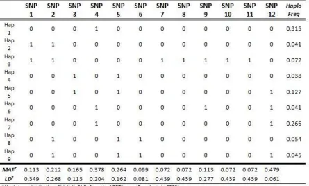
Table 2.1: Haplotype distribution with estimated SNP minor allele frequencies and linkage
disequilibrium coefficients. ... 70
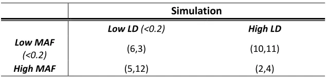
Table 2.2: Causal SNPs used in the simulation studies ... 71
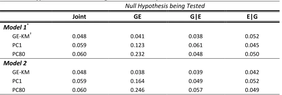
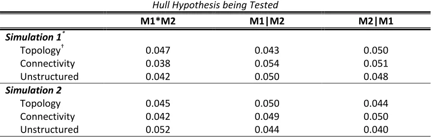
Table 2.3: Type I error rates averaged over 1000 replicate data sets ... 72
Table 2.4: Testing results from the analysis of the CoLaus Study Data ... 73
Table 3.1: Type I error rates averaged over 1000 replicate data sets ... 105
Table 3.2: Testing results from the baseline analysis of the Aspirin Data ... 106
Table 3.3: Testing results from the differential analysis of the Aspirin Data ... 107
Table 4.1: Correlation analysis between metabolic changes and drug response ... 137
Table 4.2: Pathway analysis through MetaboAnalyst 2.0 ... 138
Table 5.1: Pathway enrichment analysis of the effect of sertraline exposure from baseline to week four ... 153
Table 5.2: Correlations with treatment outcomes: correlations between biochemical ... 154
LIST OF FIGURES
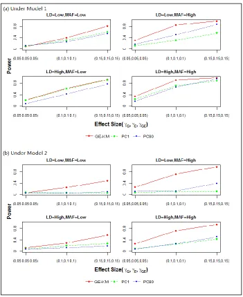
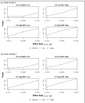
Figure 2.1: Power results for the Joint Test ... 74
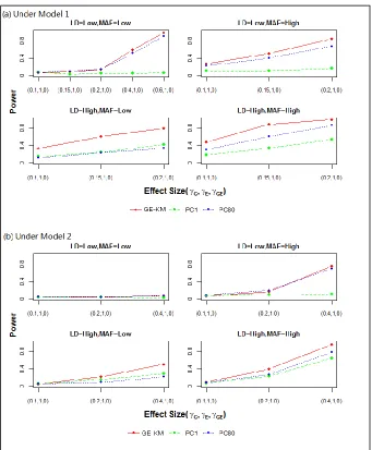
Figure 2.2: Power results for the GE Test ... 75
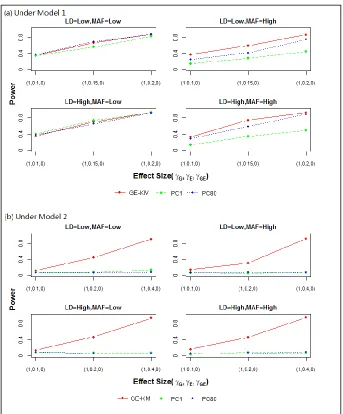
Figure 2.3: Power results for the G|E Test ... 76
Figure 2.4: Power results for the E|G Test ... 77
Figure 3.1: Modules with sale-free structures in Simulation I... 108
Figure 3.2: Modules with Non-scale-free structures in Simulation II ... 109
Figure 3.3: Power results for Simulation I (scale-free structure) when causal nodes are hub nodes ... 110
Figure 3.4: Power results for simulation I (scale-free structure) when causal nodes are random nodes ... 111
Figure 3.5: Power results for simulation II (non-scale-free structure) when causal nodes are hub nodes ... 112
Figure 3.6: Power results for simulation II (non-scale-free) when causal nodes are random nodes ... 113
Figure 4.1: The overview of module based pipeline... 139
Figure 4.2: Cluster dendrogram of metabolic changes ... 140
Figure 4.3: Pathway analysis through KEGG Mapper. ... 141
Chapter 1
Introduction
1.1 Omics studies with features and challenges
In this section, we briefly introduce three major omics disciplines, genomics, transcriptomics and metabolomics, focusing on their scientific goals, and discuss common features and challenges in these omic studies.
1.1.1 Genomics, Transcriptomics and Metabolomics
As the whole genome sequencing technology evolves and the next generation sequencing (NGS) becomes available, denser genetic markers are able to be genotyped in high efficiency and low cost. The technology improvement permits the genomic interrogations to be extended from common SNPs to rare SNPs and other types of variants including INDELs and copy number variants (CNVs). Several diseases, e.g., epilepsy (Mefford et al., 2010), autism (Pinto et al., 2010), and schizophrenia (Stone et al., 2008), have been found to be associated with rare variants that influence gene functions.
Transcriptomic and prteomic studies. Although genome, as a complete set of DNA, contains all genetic information needed to develop and maintain the organism, it is only one component responsible for the final physical appearance of the organism (i.e., phenotypes). Therefore, researches also focus on the end products of transcriptions (i.e., transcriptome) and the end products of translations (i.e., proteome). As the products of genome, Transcriptome and proteome contain the regulatory information and can serve as indicative of gene function and activity that responsible for the phenotypes, and understanding how they are related to phenotypes can great facilitate the understanding of the biological mechanism and process. One feature that makes the studies of transcriptomics and proteomics more complicated than genomics is that their expressions changes temporally and spatially, which means the performances may differ from time to time and from cell to cell.
genes is measured and can be compared among different samples in order to detect differential expressed genes. Similarly, in proteomics, protein can also be profiled, through immunoarrays, mass spectrometry and various antibody technologies, to identify variations associated with different class of subjects or treatment groups.
Metabolomic studies. Comparing to genomic, transcriptomic and proteomic information, metabolomics, provides the closest link to phenotypes because metabolites are the end products of cellular processes and reflect the ultimate response of biology system to genetic or environment changes (Fiehn, 2002). With the aid of fast development of analytical technologies, such as mass spectrometry (MS), high-resolution nuclear magnetic resonance (NMR) spectroscopy and various compound separation techniques (Dunn and Ellis, 2005; Wishart, 2008), the compound identification becomes a straightforward and fast routine. Metabolomic studies have emerged to be the newest omics sciences, with complementary role with transcriptomics and proteomics, to understand the complex mechanisms under phenotypes.
more popular today with growing demands for deep understanding of complex diseases and related biology system.
1.1.2 Features
Omics studies share three common features. First, since omics studies aim to study the complete set of biological units including genes, proteins and metabolites, they usually deal with a very large amount of variables with relative small sample size. For example, in GWAS, the number of SNPs is typically over one million. In gene expression profiling, DNA microarray can produce about ten thousands gene expression data. In proteomics and metabolomics, a single mass spectrometry experiment can identify over one thousand proteins and metabolites.
Third, the omics variables are connected functionally via a complex network. System biology studies (Barabási and Oltvai, 2004) showed that the biological units under omics studies are connected and regulate each other as part of network. In gene regulatory network, target gene and transcriptional factor interact with each other to regulate gene expression and change cell behavior. In protein network, proteins interact with each other through physical interaction to carry out important functions in many molecule processes in the cell such as DNA replication. In metabolic network, metabolites interact with each other through enzymatic conversion to fulfill metabolism and determine cell biochemical properties. This complex network structures can be regarded as one source for the nonlinear effect of biological units discussed above.
Incorporating network structure information may also increase detectability of real association and uncover potential pathway activities.
1.1.3 Challenges
Along with opportunities, the above mentioned features of omics studies also bring several significant challenges. First, the big volume of data obtained from high-throughput profiling techniques in omics studies encounter challenges in statistical analyses and computational burdens. For example, in a typical GWAS, researchers usually begin with a whole genome scan using single SNP tests. The statistical significance level after multiple testing adjustment becomes extremely stringent and limits the power of the study. The high dimension data also impacts the performance of many classical multivariate methods. For the local methods, e.g., k-nearest neighbor and local regression, which attempt to model in small neighborhoods, will run into problems in high dimension due to very sparse density of samples in the input space (Trevor et al., 2001). For the global methods, e.g., the standard least squares regression, the overcome of high dimension usually requires a sufficient large sample size which is not applicable in practice as features p is larger than the number of observations n (p>>n).
require implicit specification of the relationship between basic bio-units and the phenotypes. These methods have limited power when a model is not correctly specified to capture the underlying effects, or encounter the curse of dimensionality when include higher order terms to model complex effects.
The third challenge in omics data for utilizing network information remains in two aspects, network reconstruction and incorporation. For network reconstruction, although network structure can be reconstructed from existing biological knowledge (e.g., KEGG) or from the data (e.g., co-expressed gene modules), enormous number of potential network structures generated by network reconstruction methods tends to provide inconsistent and misleading information. For network incorporation, many methods, such as gene set enrichment analysis, have been developed to incorporate the “membership” of pathway information (i.e., belonging or not to a pathway) and demonstrated their usefulness. However, these methods do not consider the structure information that depicts the specific functional relationships among biological units.
1.2 Module based analysis in omics data
The biomarkers work jointly or even interact with each other within a complex network (Zhu et al., 2007). Consequently, biomarkers tend to have moderate individual effects but significant aggregate effect, and performing analysis at module level can increase the detectability and reproducibility of association findings. By assessing biomarker effects in a functional context, e.g., pathways and biological processes, MBA also improves the interpretability of findings and facilitates the construction of follow-up biological hypotheses. Finally, for exploratory “omics” studies, which usually begin with a full scan of a long list of candidate biomarkers, MBA provides a natural way to reduce the total number of tests, and hence relax the multiple-testing burdens and improve power.
Module based analysis is a two-step procedure including module construction and assessing module effect. We briefly discuss each step in the next sections.
1.2.1 Module construction
Module construction approaches can be generally classified into two types depending on whether or not to use prior biological knowledge. We refer the two types as expert-defined module construction and data-driven module construction approach.
elements that are known to be related to the phenotype of interest, e.g. diseases, are important targets and worth more attention. Although the field of metabolomics is relatively new, there already exist abundant databases storing hundreds of known metabolomic sets and pathways including Human Metabolome Database (HMDB) (Wishart et al., 2009), Metabolic Information Center (MIC), Specialized Metabolic Pathway Databases (SMPDB) (Frolkis et al., 2010), and Kyoto Encyclopedia of Genes and Genomes (KEGG) (Kanehisa and Goto, 1998). Additionally, tens of initial metabolomic signatures have been reported for many diseases as well, including Alzheimer’s disease (Han et al., 2002), hypertension (Brindle et al., 2003), motor neuron disease (Rozen et al., 2005), depression (Paige et al., 2006), schizophrenia (Holmes et al., 2006; Kaddurah-Daouk et al., 2007), cardiovascular and coronary artery disease (Sabatine et al., 2005), Huntington’s disease (Underwood et al., 2006), subarachnoid hemorrhage (Dunne et al., 2005), preeclampsia (Kenny et al., 2005), type 2 diabetes (Wang et al., 2005; Yuan et al., 2007), liver cancer (Yang et al., 2004), ovarian cancer (Odunsi et al., 2004), and breast cancer (Fang et al., 2005).
with the aid of known biological context, it greatly facilitates functional interpretation of testing results as well as further hypotheses generation for understanding underlying system. For example, finding a module grouping form the GO consortium (Harris et al. 2004) with clear defined attributes, such as signal transduction, not only implies a direct association between a specific biological process and the phenotype, but also provides great recourses, such as the concrete multi-level information, for understanding the biology system and generating further meaningful hypotheses.
1.2.2 Module effects assessment
In this section, we will review methods that are available for detecting module association in the context of gene-set analysis and discuss their pros and cons. We note that in this dissertation, modules are not limited to gene sets and can be any predefined sets of biological units in the omics studies.
Over-representation analysis
This approach is widely used because its simplicity and reasonability. Many authors have presented it with minor differences (Khatri and Draghici, 2005). However it has three major drawbacks. First, the chosen of top genes is based on an arbitrary threshold, which distinguishes associated genes from the rest. It’s demonstrated that different thresholds may lead to inconsistent results. Besides, the arbitrary threshold also prevents many causal genes with moderate level of association from being used to identify significant gene sets. Second, genes with different levels of association are equally treated. It causes loss of information, especially, when the levels have a wide range. Third, this method doesn’t consider the correlation structure of metabolite sets, which is important for estimating statistical significance and increasing power.
Gene set enrichment analysis (GSEA)
particular, Instead of just counting the number of set involved genes at the top of the list, ES is calculated by walking down the entire ranked list. When encountering a gene in set, the ES is increased. Otherwise, ES is decreased. The increasing amount depends on the previous calculated correlation of the gene with the phenotype. This enrichment score essentially corresponds to a weighted Kolmogorov-Smirnov-like statistic (Hollander and Wolfe, 1999); third, a null distribution of ES is generated based on the permutation of phenotype labels. And the empirical, nominal P value is then calculated; finally, the adjustment is applied to account for multiple testing of an entire database of gene sets. The size of the set has been accounted which leads to a normalized enrichment score (NSE). False discovery rate (FDR) (Benjamini et al., 2001) is estimated based on each NSE.
Several methods similar to GSEA have also been developed based on different enrichment scores. For example, Efron and Tibshirani (2007) developed a Gene Set Analysis (GSA) using a “maxmean” statistics and Smythe (2004) and Tian et al. (2005) introduced the averaged t-statistic for the enrichment score. Moreover, with the specific aim of discovering differential expression sets, PAGE, known as parametric analysis of gene set enrichment (Kim and Volsky, 2005), is developed for gene set enrichment analysis. It calculated fold change for genes between experimental groups at the beginning. Then, Z scores based on fold change are produced for each predefined gene sets as: , where
is the mean of fold change values of genes within predefined gene set, s the mean of total fold change values, is the size of a given gene set and is the standard deviation of total fold change values. Normal distribution is presumed for statistical inference based on Z score. Since PAGE doesn’t need permutation distribution, it requires much less computational effort. Additionally, simulations in their study showed PAGE was statistically more sensitive than GSEA.
Combined statistic
of individual p-values. In order to improve the power, two concepts can be incorporated into to the combined statistic: truncation and weighting. Truncation indicates pre-selection of genes based on their p values, for example, using all genes with p values below a threshold or top genes with smallest p values. Weighting indicates the weight given to each p value when combing them to the combined statistic. Since, in practice, the assumption that each gene in the set is exchangeable is always violated, these weights can be used to include the prior information about the correlation of these genes or their relative functional importance. After the combined statistic is calculated, the set-specific p-value is obtained through permutation. For the details of implementation, see De la Cruz et al. (2010).
permutation of phenotype labels. And the P value is then calculated. In case of multiple gene sets, q-values based on false discovery rates (FDRs) can be used in SAMGS.
One major disadvantage of approaches based on combined statistics is they only use all marginal effects of genes without account for the interaction effects within the gene set.
Methods using linear models
Followings are another set of approaches, which don’t rely on the individual gene tests, to jointly model the effect of all genes within a set.
One simple implementation to assess the gene-set effect is using a traditional multiple regression. Regressing phenotype (Y) on genes within given set. Then a joint test of the null hypothesis H0: reflects the association of the phenotype with given set, where m is the number of genes within given set, and β is regression coefficient. The alternative hypothesis is at least one of the coefficients differs from zero. However, in most cases, it’s unable to test the hypothesis because m might be large relative to the sample size. So the global test using random effects to fit genes within a given set is proposed by Goeman et al. (2004). Using the random linear model, Y is modeled as
When the number of genes in gene set exceeds the sample size, principal component based regression (PCR) is another commonly used approach (Tomfohr et al., 2007). It’s a two-stage approach. First, principal component analysis (PCA) is applied on target gene set to generate principal components that are linear combinations of the original variables. In common practice (Chen et al., 2008; Ma and Kosorok, 2009), either the first principle component or components exceeding certain threshold in terms of explained variance is chosen. Other rules are also developed for choosing the number of components, p, including Zhu’s method (Zhu and Ghodsi, 2006), Average Eigenvalue Rules (Peres-Neto et al., 2005) and Bartlett’s test (Bartlett, 1954; Jackson, 1993). Next, these reduced components are fitted in a regression model. Similar hypothesis testing for the effect of all the principle components, which indicates association between gene set and phenotype, is performed. One advantage of PCR is that it solves the m>n problem by choosing p where p<<m. Another advantage is when strong correlations exist among genes (predictor variables), PCR achieves better performance than ordinary linear regression.
removing variance in the X matrix not correlated to Y. However, some studies (Tapp and Kemsley, 2009) showed OPLS methods will never outperform PLS methods in terms of prediction. PCA and PLS based methods is the most widely used approaches in metabolomics data analysis. And SIMCA-P (Umetrics) implementing these methods with a very nicely designed graphical user interface and visualizations is also becoming the most widely used tool in metabolomics community.
Discussion
Numerous methods have been developed for testing the association of the gene set with phenotypes of interest. However, according to Tian et al. (2005), two distinctive null hypotheses are formulated. The first null hypothesis (Q1) is assuming the genes in the gene set show the same pattern of associations with the phenotype compared with the rest of the genes. The second hull hypothesis (Q2) is assuming no genes in the gene set associated with phenotype, which doesn’t consider the genes outside the gene set. Geoman and Buhlmann (2007) termed methods based on Q1 and Q2 as competitive and self-contained methods. According to this classification, ORA and PAGE are competitive methods while combined statistic methods including SAMGS and methods based on linear models are self-contained methods. Because of the strong null hypothesis of self-self-contained methods, only a single significantly associated gene (SAG) can cause the whole gene set significant. Consequently, they usually have more power than competitive test and can provide very powerful predictions. However, this significant gene set may not be really enriched with SAGs. Therefore, Nam and Kim (2008) confirmed a ground rule for choosing gene set methods. If the goal is to find gene sets enriched with SAGs, a competitive method fits better. Otherwise, if the goal is to find gene sets associated with phenotype, a self-contained method should be used.
different type of method as it tests another kind of hypothesis that there is no gene sets associated with the phenotype (Q3) (Nam and Kim, 2008). It targets the entire dataset and tests if any gene set in the whole dataset is associated with phenotype. In the GSEA, the enrichment score (ES) for each gene set is a competitive statistic as it summarized the relative enrichment considering genes both within predefined gene set and the rest of genes. Then, the step of sample permutation to test the significant of the entire dataset is self-contained as it assumes no gene sets in the entire dataset (set of gene sets) associated with phenotype.
One extension of traditional gene-set methods can be achieved by incorporating network structure information in order to increase the efficiency in estimation and inference on gene sets. The sensitivity of detecting relevant gene sets/pathways can be improved by incorporating pathway topology information, demonstrated by Rahnenhurer et al. (2004). SAFE, significance analysis of function and expression, presented by Barry et al. (2005), is a permutation based procedure and considers the underlying network structure. Wei and Li (2007) proposed a Markov random field model incorporating the information on the gene network in the analysis. In proteomic data, Sanguinetti et al. (2008) presented a mixture model on graphs (MMG) to account for network information and used a simple percolation algorithm to search for sub-networks of significant components. Shojaie and Michailidis (2009) used a latent variable model to incorporate network information and test whether a priori defined gene sets are differentially expressed by mixed linear models (MLM).
Thus, identifying gene-set interaction and its association with complex phenotype is crucial for characterizing underlying biological mechanisms in system biology.
1.3 Dissertations contributions and organization
1.3.1 Complete Effect-Profile Assessment in Association Studies with
Multiple Genetic and Multiple Environmental Factors
currently available across a wide range of scenarios, including varying effect size, mean model structure, and interaction complexity, which could be encountered in a Multi-G-Multi-E setting. The largest gain in power was observed when the underlying effect structure was involved complex GE interactions, suggesting that the proposed method could be a useful and powerful tool for performing exploratory or confirmatory analyses in GE-GWAS.
1.3.2 Module-based Association Analysis for Evaluating Effects of
Biomarkers with Network Structures
effects of multiple modules and their interactions with incorporating the network structure information of each module. Specifically, we developed two versions of network kernels through a unified procedure to incorporate the network structure information from different aspects. Simulation studies and an analysis of metabolic data demonstrate that our proposed methods with network information can have markedly improved power over the approach ignoring network information for investigating module effects as well as their interactions.
1.3.3 A Module-based Pipeline for Mining of Pharmacometabolomics
Data
pharmacometabolomics including identification of drug-related alternations in metabolic pathways and baseline drug response predictive signatures.
1.3.4 Pharmacometabolomics Studies of Major Depressive Disorder
(MDD)
In Chapter 5, we introduce two pharmacometabolomics studies related to major depressive disorder (MDD), in which we have been involved and identified preliminary biological signatures for the disease and drug response mechanisms.
1.4 References
Altshuler, D., Hirschhorn, J. N., Klannemark, M., Lindgren, C. M., Vohl, M. C., Nemesh, J., ... & Lander, E. S. (2000). The common PPARγ Pro12Ala polymorphism is associated with decreased risk of type 2 diabetes. Nature genetics, 26(1), 76-80.
Fridley, B. L., Jenkins, G. D., & Biernacka, J. M. (2010). Self-contained gene-set analysis of expression data: an evaluation of existing and novel methods. PLoS One, 5(9), e12693.
Barabási, A. L., & Oltvai, Z. N. (2004). Network biology: understanding the cell's functional organization. Nature Reviews Genetics, 5(2), 101-113.
Bartlett, M. S. (1954). A note on the multiplying factors for various χ 2 approximations. Journal of the Royal Statistical Society. Series B (Methodological), 296-298.
Bechtel, W., Richardson, R. C., & Sloan, P. R. (1994). Discovering complexity: Decomposition and localization as strategies in scientific research. ISIS-International Review Devoted to the History of Science and its Cultural Influence, 85(4), 746-746.
Benjamini, Y., Drai, D., Elmer, G., Kafkafi, N., & Golani, I. (2001). Controlling the false discovery rate in behavior genetics research. Behavioural brain research, 125(1), 279-284.
Benjamini, Y., & Hochberg, Y. (1995). Controlling the false discovery rate: a practical and powerful approach to multiple testing. Journal of the Royal Statistical Society. Series B (Methodological), 289-300.
Brindle, J. T., Nicholson, J. K., Schofield, P. M., Grainger, D. J., & Holmes, E. (2003). Application of chemometrics to 1H NMR spectroscopic data to investigate a relationship between human serum metabolic profiles and hypertension. Analyst, 128(1), 32-36.
Brindle, J. T., Antti, H., Holmes, E., Tranter, G., Nicholson, J. K., Bethell, H. W., ... & Grainger, D. J. (2002). Rapid and noninvasive diagnosis of the presence and severity of coronary heart disease using 1H-NMR-based metabonomics. Nature medicine, 8(12), 1439-1445.
Cirulli, E. T., & Goldstein, D. B. (2010). Uncovering the roles of rare variants in common disease through whole-genome sequencing. Nature Reviews Genetics,11(6), 415-425.
Liu, D., Lin, X., & Ghosh, D. (2007). Semiparametric Regression of Multidimensional Genetic Pathway Data: Least‐Squares Kernel Machines and Linear Mixed Models. Biometrics, 63(4), 1079-1088.
De la Cruz, O., Wen, X., Ke, B., Song, M., & Nicolae, D. L. (2010). Gene, region and pathway level analyses in whole‐genome studies. Genetic epidemiology, 34(3), 222-231. Dinu, I., Liu, Q., Potter, J. D., Adewale, A. J., Jhangri, G. S., Mueller, T., ... & Yasui, Y. (2008). A
biological evaluation of six gene set analysis methods for identification of differentially expressed pathways in microarray data.Cancer informatics, 6, 357. Dinu, I., Potter, J. D., Mueller, T., Liu, Q., Adewale, A. J., Jhangri, G. S., ... & Yasui, Y. (2007).
Improving gene set analysis of microarray data by SAM-GS. BMC bioinformatics, 8(1), 242.
Doris, P. A. (2002). Hypertension genetics, single nucleotide polymorphisms, and the common disease: common variant hypothesis. Hypertension, 39(2), 323-331.
Dunn, W.B. & Ellis, D.I. (2005). Metabolomics: current analytical platforms and methodologies. Trends Analyt. Chem, 24, 285–294.
Dunne, V. G., Bhattachayya, S., Besser, M., Rae, C., & Griffin, J. L. (2005). Metabolites from cerebrospinal fluid in aneurysmal subarachnoid haemorrhage correlate with vasospasm and clinical outcome: a pattern‐recognition 1H NMR study. NMR in Biomedicine, 18(1), 24-33.
Fan, X., Ba, J., & Shen, P. (2006, January). Diagnosis of breast cancer using HPLC metabonomics fingerprints coupled with computational methods. InEngineering in Medicine and Biology Society, 2005. IEEE-EMBS 2005. 27th Annual International Conference of the (pp. 6081-6084). IEEE.
Fisher, R. A. (1922). On the interpretation of χ 2 from contingency tables, and the calculation of P. Journal of the Royal Statistical Society, 85(1), 87-94.
Fisher, S. R. A. (1970). Statistical methods for research workers (Vol. 14, pp. 140-142). Edinburgh: Oliver and Boyd.
Frazer, K. A., Murray, S. S., Schork, N. J., & Topol, E. J. (2009). Human genetic variation and its contribution to complex traits. Nature Reviews Genetics, 10(4), 241-251.
Frolkis, A., Knox, C., Lim, E., Jewison, T., Law, V., Hau, D. D., ... & Wishart, D. S. (2010). SMPDB: the small molecule pathway database. Nucleic Acids Research, 38(suppl 1), D480-D487.
Geladi, P., & Kowalski, B. R. (1986). Partial least-squares regression: a tutorial. Analytica Chimica acta, 185, 1-17.
Goeman, J. J., & Bühlmann, P. (2007). Analyzing gene expression data in terms of gene sets: methodological issues. Bioinformatics, 23(8), 980-987.
Goeman, J. J., Van De Geer, S. A., De Kort, F., & Van Houwelingen, H. C. (2004). A global test for groups of genes: testing association with a clinical outcome. Bioinformatics, 20(1), 93-99.
Harris, M. A., Clark, J., Ireland, A., Lomax, J., Ashburner, M., Foulger, R., ... & Gwinn, M. (2004). The Gene Ontology (GO) database and informatics resource. Nucleic Acids Research, 32(Database issue), D258-61.
Hollander, M. & Wolfe, D. A. (1999). Nonparametric Statistical Methods. New York: Wiley. Series B (Methodological) ,57 (1), 289–300.
Holmes, E., Tsang, T. M., Huang, J. T. J., Leweke, F. M., Koethe, D., Gerth, C. W., ... & Bahn, S. (2006). Metabolic profiling of CSF: evidence that early intervention may impact on disease progression and outcome in schizophrenia. PLoS medicine, 3(8), e327.
Jackson, D. A. (1993). Stopping rules in principal components analysis: a comparison of heuristical and statistical approaches. Ecology, 2204-2214.
Kaddurah-Daouk, R., McEvoy, J., Baillie, R. A., Lee, D., Yao, J. K., Doraiswamy, P. M., & Krishnan, K. R. R. (2007). Metabolomic mapping of atypical antipsychotic effects in schizophrenia. Molecular psychiatry, 12(10), 934-945.
Kanehisa, M. & Goto, S. KEGG, (1998). Kyoto encyclopedia of genes and genomes. Nucleic Acids Res, 28, 27– 30.
Kenny, L. C., Dunn, W. B., Ellis, D. I., Myers, J., Baker, P. N., & Kell, D. B. (2005). Novel biomarkers for pre-eclampsia detected using metabolomics and machine learning. Metabolomics, 1(3), 227-234.
Khatri, P., & Drăghici, S. (2005). Ontological analysis of gene expression data: current tools, limitations, and open problems. Bioinformatics, 21(18), 3587-3595.
Klein, R. J., Zeiss, C., Chew, E. Y., Tsai, J. Y., Sackler, R. S., Haynes, C., ... & Hoh, J. (2005). Complement factor H polymorphism in age-related macular degeneration. Science, 308(5720), 385-389.
Kraft, P., Yen, Y. C., Stram, D. O., Morrison, J., & Gauderman, W. J. (2007). Exploiting gene-environment interaction to detect genetic associations. Human heredity, 63(2), 111-119.
Kwee, L. C., Liu, D., Lin, X., Ghosh, D., & Epstein, M. P. (2008). A powerful and flexible multilocus association test for quantitative traits. The American Journal of Human Genetics, 82(2), 386-397.Lee, M. L. T., Kuo, F. C., Whitmore, G. A., & Sklar, J. (2000). Importance of replication in microarray gene expression studies: statistical methods and evidence from repetitive cDNA hybridizations. Proceedings of the National Academy of Sciences, 97(18), 9834-9839.
Li, C., & Li, H. (2008). Network-constrained regularization and variable selection for analysis of genomic data. Bioinformatics, 24(9), 1175-1182.
Liu, Q., Dinu, I., Adewale, A., Potter, J., & Yasui, Y. (2007). Comparative evaluation of gene-set analysis methods. BMC bioinformatics, 8(1), 431.
Wu, M. C., Kraft, P., Epstein, M. P., Taylor, D. M., Chanock, S. J., Hunter, D. J., & Lin, X. (2010). Powerful SNP-set analysis for case-control genome-wide association studies. The American Journal of Human Genetics, 86(6), 929-942.
Ma, S., & Kosorok, M. R. (2009). Identification of differential gene pathways with principal component analysis. Bioinformatics, 25(7), 882-889.
Mefford, H. C., Muhle, H., Ostertag, P., von Spiczak, S., Buysse, K., Baker, C., ... & Eichler, E. E. (2010). Genome-wide copy number variation in epilepsy: novel susceptibility loci in idiopathic generalized and focal epilepsies. PLoS Genetics, 6(5), e1000962.
Moore, J. H., Asselbergs, F. W., & Williams, S. M. (2010). Bioinformatics challenges for genome-wide association studies. Bioinformatics, 26(4), 445-455.
Mootha, V. K., Lindgren, C. M., Eriksson, K. F., Subramanian, A., Sihag, S., Lehar, J., ... & Groop, L. C. (2003). PGC-1α-responsive genes involved in oxidative phosphorylation are coordinately downregulated in human diabetes. Nature Genetics, 34(3), 267-273.
Murcray, C. E., Lewinger, J. P., & Gauderman, W. J. (2009). Gene-environment interaction in genome-wide association studies. American journal of epidemiology, 169(2), 219-226.
Naj, A. C., Jun, G., Beecham, G. W., Wang, L. S., Vardarajan, B. N., Buros, J., ... & DeCarli, C. (2011). Common variants at MS4A4/MS4A6E, CD2AP, CD33 and EPHA1 are associated with late-onset Alzheimer's disease. Nature Genetics, 43(5), 436-441. Nam, D., & Kim, S. Y. (2008). Gene-set approach for expression pattern analysis. Briefings in
bioinformatics, 9(3), 189-197.
Fiehn, O. (2002). Metabolomics–the link between genotypes and phenotypes. Plant molecular biology, 48(1-2), 155-171.
Paige, L. A., Mitchell, M. W., Krishnan, K. R. R., Kaddurah‐Daouk, R., & Steffens, D. C. (2007). A preliminary metabolomic analysis of older adults with and without depression. International journal of geriatric psychiatry,22(5), 418-423.
Peres-Neto, P. R., Jackson, D. A., & Somers, K. M. (2005). How many principal components? Stopping rules for determining the number of non-trivial axes revisited. Computational Statistics & Data Analysis, 49(4), 974-997.
Pérez-Enciso, M., & Tenenhaus, M. (2003). Prediction of clinical outcome with microarray data: a partial least squares discriminant analysis (PLS-DA) approach. Human genetics, 112(5-6), 581-592.
Pinto, D., Pagnamenta, A. T., Klei, L., Anney, R., Merico, D., Regan, R., ... & Green, A. (2010). Functional impact of global rare copy number variation in autism spectrum disorders. Nature, 466(7304), 368-372.
Rahnenfuhrer, J., Domingues, F. S., Maydt, J., & Lengauer, T. (2004). Calculating the statistical significance of changes in pathway activity from gene expression data. Statistical Applications in Genetics and Molecular Biology, 3(1), 1055.
Rozen, S., Cudkowicz, M. E., Bogdanov, M., Matson, W. R., Kristal, B. S., Beecher, C., ... & Kaddurah-Daouk, R. (2005). Metabolomic analysis and signatures in motor neuron disease. Metabolomics, 1(2), 101-108.
Sabatine, M. S., Liu, E., Morrow, D. A., Heller, E., McCarroll, R., Wiegand, R., ... & Gerszten, R. E. (2005). Metabolomic identification of novel biomarkers of myocardial ischemia. Circulation, 112(25), 3868-3875.
Shojaie, A., & Michailidis, G. (2009). Analysis of gene sets based on the underlying regulatory network. Journal of Computational Biology, 16(3), 407-426.
Smyth, G. K. (2004). Linear models and empirical bayes methods for assessing differential expression in microarray experiments. Stat Appl Genet Mol Biol, 3(1), 3.
Stone, J. L., O’Donovan, M. C., Gurling, H., Kirov, G. K., Blackwood, D. H., Corvin, A., ... & Kwan, S. L. (2008). Rare chromosomal deletions and duplications increase risk of schizophrenia. Nature, 455(7210), 237-241.
Strange, K. (2005). The end of “naïve reductionism”: rise of systems biology or renaissance of physiology?. American Journal of Physiology-Cell Physiology, 288(5), C968-C974. Subramanian, A., Tamayo, P., Mootha, V. K., Mukherjee, S., Ebert, B. L., Gillette, M. A., ... &
Mesirov, J. P. (2005). Gene set enrichment analysis: a knowledge-based approach for interpreting genome-wide expression profiles. Proceedings of the National Academy of Sciences of the United States of America, 102(43), 15545-15550.
Thomas, D. (2010)a. Gene–environment-wide association studies: emerging approaches. Nature Reviews Genetics, 11(4), 259-272.
Thomas, D. (2010)b. Methods for investigating gene-environment interactions in candidate pathway and genome-wide association studies. Annual review of public health, 31, 21.
Thornton-Wells, T. A., Moore, J. H., & Haines, J. L. (2004). Genetics, statistics and human disease: analytical retooling for complexity. TRENDS in Genetics, 20(12), 640-647. Tian, L., Greenberg, S. A., Kong, S. W., Altschuler, J., Kohane, I. S., & Park, P. J. (2005).
Tomfohr, J., Lu, J., & Kepler, T. B. (2005). Pathway level analysis of gene expression using singular value decomposition. BMC bioinformatics, 6(1), 225.
Trevor. Hastie, Robert. Tibshirani, & Friedman, J. J. H. (2001). The elements of statistical learning (Vol. 1). New York: Springer.
Trygg, J., & Wold, S. (2002). Orthogonal projections to latent structures (O‐PLS). Journal of Chemometrics, 16(3), 119-128.
Underwood, B. R., Broadhurst, D., Dunn, W. B., Ellis, D. I., Michell, A. W., Vacher, C., ... & Rubinsztein, D. C. (2006). Huntington disease patients and transgenic mice have similar pro-catabolic serum metabolite profiles. Brain,129(4), 877-886.
Wang, C., Kong, H., Guan, Y., Yang, J., Gu, J., Yang, S., & Xu, G. (2005). Plasma phospholipid metabolic profiling and biomarkers of type 2 diabetes mellitus based on high-performance liquid chromatography/electrospray mass spectrometry and multivariate statistical analysis. Analytical Chemistry, 77(13), 4108-4116.
Wang, Z., Gerstein, M., & Snyder, M. (2009). RNA-Seq: a revolutionary tool for transcriptomics. Nature Reviews Genetics, 10(1), 57-63.
Wei, Z., & Li, H. (2007). A Markov random field model for network-based analysis of genomic data. Bioinformatics, 23(12), 1537-1544.
Wishart, D. S., Knox, C., Guo, A. C., Eisner, R., Young, N., Gautam, B., ... & Forsythe, I. (2009). HMDB: a knowledgebase for the human metabolome. Nucleic Acids Research, 37(suppl 1), D603-D610.
Wishart, D.S. (2008). Quantitative metabolomics using NMR. Trends Analyt. Chem, 27, 228– 237.
Yang, J., Xu, G., Zheng, Y., Kong, H., Pang, T., Lv, S., & Yang, Q. (2004). Diagnosis of liver cancer using HPLC-based metabonomics avoiding false-positive result from hepatitis and hepatocirrhosis diseases. Journal of Chromatography B, 813(1), 59-65.
Yuan, K., Kong, H., Guan, Y., Yang, J., & Xu, G. (2007). A GC-based metabonomics investigation of type 2 diabetes by organic acids metabolic profile. Journal of Chromatography B, 850(1), 236-240.
Zhu, M., & Ghodsi, A. (2006). Automatic dimensionality selection from the scree plot via the use of profile likelihood. Computational Statistics & Data Analysis, 51(2), 918-930. Zhu, X., Gerstein, M., & Snyder, M. (2007). Getting connected: analysis and principles of
Chapter 2
Complete Effect-Profile Assessment in
Association Studies with Multiple Genetic
and Multiple Environmental Factors
Zhi Wang1,*, Megan L. Neely2,*, Arnab Maity3, Jung-Ying Tzeng1,3,4
1: Bioinformatics Research Center, North Carolina State University, Raleigh NC, 27695, USA 2: Department of Biostatistics and Bioinformatics, Duke University, Durham, NC, 27705, USA 3: Department of Statistics, North Carolina State University, Raleigh NC, 27695, USA
2.1 Abstract
KEYWORDS: factor-set association analysis; kernel machine regression; GWAS; genetic-environmental interactions; joint and conditional tests.
2.2 Introduction
Complex human diseases are influenced not only by genetic and environmental factors but also by the interplay between the two. Investigating gene-environment (GE) interactions can facilitate understanding the etiology of these phenotypes by providing insight into biological mechanisms associated with diseases [Murcray et al., 2009; Mechanic et al., 2012], by explaining heterogeneity across populations, by classifying risk subgroups based on differential environmental exposures [Kraft et al., 2007; Murcary et al., 2009; Thomas, 2010a, 2010b], and by identifying novel genes acting through interactions but exhibiting minimal marginal effects [Thomas, 2010a].
by the emergence of Multi-G-Multi-E studies in the recent literature [Wu et al., 2012; Dai et al. 2013; Edwards et al., 2013; Naj et al., 2013; Patel et al., 2013].
Approaches currently available for examining effect profiles in Multi-G-Multi-E analyses include naïve regression, principal component (PC) regression, and kernel machine (KM) regression. Naïve regression investigates the relationship between the genetic and environmental factor-sets and the response by treating each element of the factor-sets as an individual covariate in a regression model and then performing significance testing. PC regression first performs principal component analysis on the genetic and environmental factor-sets and then uses a subset of the resulting principle components (e.g., the first PC or the top PCs that explain 80% of the variation in the set) in a regression analysis [Gauderman et al., 2007; Wang et al., 2009]. Investigating GE interactions can easily be incorporated into these frameworks, but there are several potential drawbacks to using these approaches in the Multi-G-Multi-E setting. Naïve regression is straight forward and easy to apply, but is usually under powered due to the large number of predictors and the small effect sizes of individual factors [Wu et al., 2010; Lin et al., 2011]. While PC regression typically has better power than naïve regression, its application can be subjective when deciding how many PCs to include in the downstream analyses and valuable information can be lost. Moreover, naïve and PC regression do not incorporate any prior information about the elements of the factor-sets.
function and then performs least squares regression of the response on the similarity measures. Thus, if the number of parameters in the model is more than the number of subjects, KM regression can be thought of as a dimension reduction technique. Even if the actual number of variables (e.g., the number of genetic and environmental factors) is less than the sample size, the number of parameters can still exceed the sample size if higher order main or interaction effects are considered in the mean model. In the KM framework, testing for the factor set effects is reduced to testing for the nullity of the corresponding variance components rather than the actual parameters in the mean model. Typically, the corresponding degrees of freedom used by the KM test are much smaller than the number of model parameters, resulting in increased power [Liu et al., 2007; Kwee et al., 2008; Liu et al., 2008]. KM regression does not suffer from the burden of dimensionality like naïve regression, less information is lost to data-reduction compared to PC regression, and kernels can be constructed to incorporate important biological information [Kwee et al., 2008; Wu et al., 2010]. In addition, KM regression can handle correlated factors like PC regression and allows for the investigation of non-linear effects, which is not practical in naïve regression and not feasible in PC regression.
examines the interaction between a single environmental factor and a set of genetic markers. While this approach can be used to directly test for GE interaction, only a single environmental can be considered at a time rather than an environmental factor-set. Wu and Maity [personal communication] are in the process of developing a KM regression approach that attempts to separate the individual genetic (G) and environmental (E) effects from the combined joint effect through careful modeling. Then, using the remaining signal to capture the GE interaction effect, they attempt to build a test based on this component, avoiding the need to specify any explicit kernel for the GE interaction.
of simulation studies designed to compare its performance to currently available approaches, present an application of our method to data from a cardiovascular disease study, and conclude with a brief discussion of the work’s major findings and connections to the current literature.
2.3 Methods
Let the vector represent the observed data for individual in a sample of size . Let represent the continuous trait value. Let be a vector containing un-phased genotypes at biallelic SNPs. Let be a vector containing environmental factors. Let be a vector containing covariates that are not included in either or .
Using a linear regression model, the relationship between the continuous trait value and the genetic factors , the environmental factors , and their interactions , after adjusting for the additional covariates , can be characterized as
where is a vector of regression coefficients describing the effects of the covariates , ’s are independent random errors that follow a distribution, and
which has been shown to perform well in the Multi-G or Multi-E settings where high-dimensionality and highly correlated covariates are often present [Liu et al., 2007; Kwee et al., 2008; Liu et al., 2008].
Under the KM framework, can be specified through a linear combination of a positive definite kernel function and is assumed to lie in the functional space generated by that kernel [Kimeldorf and Wahba, 1970; Liu et al., 2008]. Following the representation theorem, the functions and in the linear regression model in (1) can be written as ,
, and , respectively, where are the unknown parameters. The kernel function is a distance metric that quantifies the similarity between subject and subject . Some commonly used kernel functions include the linear kernel function, given by
, the IBS kernel for genetic data, given below in (2), and the polynomial kernel function, given by .
2.3.1 GE Interaction Kernel
In this work, we aim to design a kernel function that can be used to model high-dimensional, complex interactions between genetic and environmental factors in a Multi-G-Multi-E setting. We propose that a GE kernel, denoted by , can be appropriately constructed as a function of the chosen genetic and environmental kernels, denoted by
effects) allowing a GE analysis under the KM framework to enjoy the same ease-of-interpretation as a naïve regression or a PC regression analysis where each component of the effect profile can readily be focused on inferentially.
For the genetic kernel, we selected the IBS kernel that is commonly used for genotype data [Kwee et al., 2008] and is given by
where denotes the number of alleles shared by subject and subject at SNP and are SNP-specific weights. The weights are used to incorporate prior information about the genetic variants into the analysis in order to improve performance. Because similarity in rare alleles is more informative than similarity in common alleles, we took the weights to be
as recommended by Pongpanich et al. [2012], where is the minor allele frequency (MAF) of SNP . With this weight, the contribution of rare variants is up-weighted, but not too strongly so that the contribution of common variants can still be retained. For the environmental kernel, we selected the interactive kernel [Maity and Lin, 2011] given by
which explicitly includes two-way interactions along with the main effects of the environmental variables. If one wishes to include quadratic effects in the model, then the 2nd-order polynomial kernel can be specified instead.
Finally, we construct a GE kernel based on the selected genetic and environmental kernels. Direct construction of a GE kernel based on commonly used genetic and environmental kernels is not a straightforward task due to the concern of introducing duplicate terms in the GE kernel. That is, when constructing as a function of and , marginal genetic and environmental effects often appear in that are already captured in or . For example, in our setting, if we constructed as the product of and , the GE kernel would be defined as
The duplicate genetic main effect term is introduced by the constant in the interaction kernel used for the environmental kernel. The presence of duplicate terms in the GE kernel causes colinearity and leads to invalid conclusion about the interaction effects. The overlap in (4) suggests a simple yet effective solution for directly constructing the GE kernel using the genetic and environmental kernels: re-define the environmental kernel as
The approach in (5) can also be used for general kernel specification. For example, if one chooses to use a polynomial kernel for or instead of the IBS or interaction kernel, respectively, one can define for or first, and then construct by taking the element-wise product of and .
2.3.2 Score tests for assessing Multi-G-Multi-E Effects
In a Multi-G-Multi-E setting, there may be several null hypotheses of interest depending on the goal of the analysis. For example, in a confirmatory analysis, the goal may be to replicate a GE interaction signal and the GE effect would be tested individually. However, in an exploratory analysis, the goal maybe to look for any evidence of a relationship between the genetic and environmental factors and the response and the G, E, and GE effects would be tested jointly. To address these needs, we develop a series of tests based on the linear regression model in (1).
genes can exhibit negligible marginal effects but strong effects among particular exposure groups [Kraft et al., 2007; Thomas, 2010a].
Furthermore, if there is no evidence of a GE interaction, conditional genetic and environmental effects can be further evaluated by testing without constraining but under the constraint of , and testing without constraining but under the constraint of , respectively. We develop conditional tests, and , rather than marginal tests of G or E, because they are usually more meaningful and interpretable in the context of Multi-G-Multi-E studies. That is, researchers are often interested in investigating the incremental information about the response provided by genetic effects, for example, over and above other covariates in the mean model. Additionally, the conditional tests can be used to understand the inconsistent association findings because marginal associations, often called the crude associations [Robins and Morgenstern, 1987], may disappear after taking differences in other genetic and environmental factors into consideration.
Using an argument similar to Liu et al. [2007], we show in the Supplementary Note that Model (1) has an equivalent linear mixed model representation and can be expressed as
, , , and
,
where , for ,
for , , and
. In the Supplementary Note, we also derive the EM algorithms, following similar steps as described in Tzeng et al. [2011], to obtain the estimates of the nuisance variance components (i.e., ) under certain null hypotheses. As shown in the Supplementary Note, these test statistics asymptotically follow a weighted chi-squared distribution, and p values can be obtained by moment matching approaches [Duchesne and Lafaye De Micheaux, 2010].
2.4 Simulation Studies
Our simulation studies were based on a 12-locus haplotype distribution of biallelic single nucleotide polymorphisms (SNPs) from the AGRT1 gene [French et al., 2006]. The haplotype distribution as well as the minor allele frequencies (MAFs) and linkage disequilibrium (LD) coefficients for each SNP are given in Table 2.1. The LD was quantified by the average pair-wise R2 between each SNP and the remaining 11 SNPs. We considered 2 causal loci out of the 12 SNPs under 4 scenarios (Table 2.2): the 2 causal variants had low vs. high MAFs and were in low vs. high LD.
We generated the genotypes of the 12 SNPs based on the haplotype distribution in Table I and generated 5 environmental factors from the multivariate normal distribution
where with and . The phenotype values were
generated using the model , where were generated from a distribution and two models for were considered:
Model 1 (M1) :
, and
Model 2 (M2):
1 2 1 2.
When examining the power of the Joint Test, we set for
in M1 and M2. For the GE test, we set and for
in M1 and M2. For the G|E test, we set , , and
for in M1 and in M2. For the E|G test, we set , , and for in M1 and
in M2. These effect sizes (i.e., the ’s) were chosen so that the power of detecting a signal fell within a reasonable range. When examining the type I error rate of the Joint Test, we set in M1 and M2. For the GE test, we set
and in M1 and M2. For the G|E test, we set , , and in M1 and M2. For the E|G test, we set and in M1 and M2.
Taken together, this leads to 256 distinct simulation settings that cover . In each simulation setting, samples of size 200 were generated. We generated 100 replicates for power simulations and 1000 replicates for evaluating type I error rates. Each replicate was analyzed using the following methods: (1) GE-KM: the proposed KM regression with constructed using the IBS kernel on the G set (the 12-SNP genotypes) and weights
2.5 Results
Type I error rates are presented in Table 2.3. Power results are presented in Figures 2.1 – 2.4. Each figure contains results for M1 (panel (a)) and M2 (panel (b)) and for the 4 simulation scenarios – low vs. high MAF (across columns) and low vs. high LD (down rows). Effect sizes for the causal genetic and environmental factors are shown on the x-axis. The power of each method to detect a signal, plotted as a separate line, is shown on the y-axis.
In short, KM performed similarly or better than either PC method, suggesting that GE-KM could be a powerful and flexible analytic tool in the Multi-G-Multi-E setting.
THE GE TEST. The GE test searches for a signal among the interaction between all genetic and environmental factors. In this setting, only GE-KM has a desirable performance under a null model (Table 2.3). The type I error rates for the PC methods are much higher than the nominal level. This could possibly be because the GE interaction term fitted in the PC model captured the effects of the GG and EE and led to spurious GE association. Because the type I error rates of the PC methods were so inflated, we did not consider PC methods in the power analysis of the GE test. As the effect size increased, so did the power of GE-KM. However, in order to obtain a range of power in the GE test setting similar to that of the joint test setting, the effect sizes had to be approximately doubled (see Figure 2.2). Increasing the MAF, the LD, and the complexity of the effect structure (i.e., M1 vs. M2) had minimal effects on the power of GE-KM, suggesting that the power of GE-KM may not be heavily influenced by these factors when performing the GE test. In summary, GE-KMR is able to maintain control on the type I error rate while achieving meaningful power to detect a signal.
over the PC methods resulted from increasing the LD from low to high. Under M2, the same general pattern of results was observed. However, the power gain of GE-KM over the PC methods was not as substantial, suggesting the IBS kernel may have limited power to capture interaction effects among the genetic factors. The overall power observed under M2 was markedly lower than the overall power observed under M1 even after approximately doubling the effect sizes. When both the MAF and LD are low, all three methods achieved only minimal power under M1 and M2. To help clarify the relationship, additional effect sizes were studied (i.e., 0.4 and 0.6). Under M1, increasing the effect size resulted in desirable power gains. The same was not true under M2. After reexamining the haplotype distribution, we found that there are no overlapping minor alleles between the two causal SNPs chosen for this scenario. Therefore, under M2 constructing the GG interaction always produced a zero-term which led to no genetic effects in the data generation model. In summary, the performance of all three approaches suffered in the G|E setting; yet the GE-KM performed similarly or better than the PC methods.
methods under M2, where the power remained near null across all studied effect sizes. Increasing the MAF and LD has little effect on GE-KM in this setting. These results confirm that PC methods have little capability to capture interaction effects because they only take linear effects into consideration. Conversely, the GE-KM was able to perform well even when the effect profile involved complex interactions between the G and E effects.
2.6 Real data example: Application to the CoLaus study data
We used the proposed KM regression method to analyze data from the CoLaus study [Song et al., 2011]. The data set contains the measured plasma level of the lipoprotein-associated phospholipase A2 (Lp-PLA2) enzyme in 87 subjects, which has been shown to be associated with risk of coronary heart disease. Song et al. [2011] studied the effect of the non-synonymous rare variants (MAF < 0.05) in PLA2G7 on Lp-PLA2 activity based on 29 carriers of the rare non-synonymous variants and 58 matched non-carriers who were matched based on age, sex and low-density lipoprotein cholesterol level. The study found significantly lower Lp-PLA2 activity in carriers compared to the non-carriers.