Model Updating through Measured Data in the Case of a Feed Water Pipeline (J057)

Transactions of the 17th _{International Conference on} Structural Mechanics in Reactor Technology (SMiRT 17)

Prague, Czech Republic, August 17 –22, 2003

Paper # J05-8

Model Updating through Measured Data in the Case of a Feed Water Pipeline

Arja Saarenheimo1)_{, Heikki Haapaniemi}1)_{, Pekka Luukkanen}2) _{and Pekka Nurkkala}3)

1) VTT Industrial Systems Espoo, Finland

2) Fortum Power and Heat Ltd Loviisa NPP, Finland 3) Fortum Service Vantaa, Finland

ABSTRACT

The main objective of this ongoing project is to develop practical methods for monitoring the condition and remaining lifetime of process piping. Relevant information about the actual loading state and condition of the piping can be obtained by direct measurements. Some structural details may be difficult to model properly or they may deviate from design documents. In order to get a realistic numerical model, measured data is needed in updating the finite element model. The updated numerical model can further be used in planning structural modifications or considering structural behaviour under new loading conditions. Also, optimal locations for transducers used for condition monitoring can be predicted.

Three pilot pipelines were chosen in order to study and develop the method described above. The third pilot piping system handled in this paper is a feed water pipeline, RL61, of the VVER 440 type PWR NPP Loviisa 1. The project’s tasks are modal testing, modal correlation analysis and model updating. The computational model is updated through measurements, but in practice measurements are often quite limited.

KEYWORDS

Model updating, finite element, correlation analysis, dynamical analysis, experimental model.

INTRODUCTION

The purpose of this study was to update a Finite Element (FE) model of a nuclear power plant piping system under different measurement conditions, referred to here as Boundary Conditions (BC). The main subjects discussed here are results from model updating in the case of a non-insulated and empty piping system (Case 1), and preliminary work on identifying possible modelling errors between this updated model and an experimental model in the case of changed BC (Case 3). Case 3 BC refers to situations where the piping system was filled with hot water and insulated with mineral wool. Similar analyses for identifying discrepancies between the FE model and experimental model were also performed in the case of an empty and insulated piping system (Case 2), but due to limited space those results are not discussed here.

MODEL UPDATING

The original FE model, which was also used as a base model for further updating, was based on design drawings and walk-down inspections results. The ABAQUS/Standard [1] code was used for finite element analyses. An illustration of the RL61 feed water pipeline is shown in Fig. 1. The main dimensions of the pipeline are also given. The outer diameter of the pipe is 324 mm and the pipe bend curvature 600mm. The thickness of the pipe is generally 20 mm, except for the longest vertical part, which has a wall thickness of 17.5mm. The experimental model of the Rl61 piping system along with measurement points is shown in Fig. 2. The feed water pipeline is connected to the pump at measurement point 103 and to the main feed water line at point 438. Points 326 and 330 indicate valves V1 and V2, each weighing 978 kg, at the lower part of the piping. The pipeline is supported by three spring hangers referred to in the following as S1, S2 and S3 and shown in Fig.1 numbered 46, 47 and 48, respectively. Corresponding locations in Fig. 2 are points 227, 119 and 109. The spring constant of S1 is 660 N/mm and the corresponding value for springs S2 and S3 is 446N/mm. The experimental measurements are described in more detail elsewhere [2] [3].

The first task in evaluating the quality of the original FE model was to make several comparisons using both frequency difference and Modal Assurance Criterion (MAC) values as parameters indicating the similarity between FE and experimental modes. The MAC value indicates the degree of similarity between two mode shapes; an MAC value of one means they are identical. The MAC value between analytical {ψa} and experimental {ψe} mode shape vectors is

{ } { }

{ } { }

(

)

(

{ } { }

)

2

( , )

H

e a

a e _{H H}

e e a a

MACψ ψ ψ ψ

ψ ψ ψ ψ

= , (1)

where superscript H is the Hermitian transpose, [A]H_=([A]T₎*_{, * denotes the complex conjugate. A commonly used} real-life criterion for deciding if two modes are similar is whether the MAC value is ≥ 0.7, in which case the modes correlate, or < 0.5, in which case they do not.

The results of MAC analysis are compiled into a mode pair table as shown in Table 1, from which it can be seen that the correlation between the FE model and the experimental results is far from acceptable. Especially the frequency differences seem to be very high, even if the mode shape correlation is acceptable as e.g. in the case of pair No. 1.

Figure 1. Illustration of actual RL61 feed water piping system.

2 2 2 2 2 1 2 2 0

4 3 8 2 3 6 1 1 9

1 1 8 T e st M o d e l 1 1 7

1 1 6

5 4 0 1 1 5

5 4 1 1 1 4

5 4 2 1 0 3 1 0 5 1 0 6 1 1 3

Table 1. Mode pair table between original FE model and experimental results.

Pair # FEA Freq. [Hz] EMA Freq. [Hz] Diff. [% ] MAC [%]

1 1 2.55 1 1.81 40.96 78.6

2 8 22.47 10 17.45 28.76 28.3

3 10 30.18 13 21.67 39.25 35.6

4 11 33.98 15 25.99 30.76 72.9

5 14 54.33 17 39.07 39.06 74.7

6 15 63.85 20 47.42 34.65 24.9

These results indicate that model updating is needed, and previous experiences suggest that the main effort should focus on support structures and modelling the connections to the surrounding structure correctly. First, a walk-down updating was carried out. Only some minor details were needed to modify in the FE model. A rough model of the feed water pump was added to the FE model. Measurement points 540-542 are located at the feed water pump. At the measurement model point 438 there is a T-connection to the main feed water line. Also, part of this feed water line was modelled with pipe elements. FEM tools updating code [4] was used for model updating. Because the mass of the system was believed to be modelled correctly, the updating process was carried out by modifying Young's modulus at those places where some simplifications and idealisations were made in the FE modelling. The update information concerning Young's modulus is summarised briefly in Table 2.

Table 2. Updated stiffness, difference of Young's modulus [%].

Location Connection to the

main feed water line Valves V1 and V2 Connection to the feed water pump Related nodes

in Fig. 2. 438 224, 228, 330326, 103, 105

Difference [%] 60-80 20 80

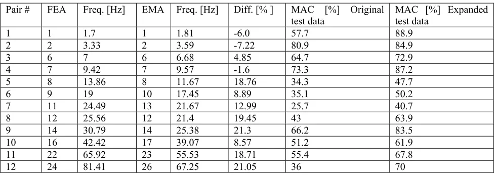
After some model-updating runs, improvement in modal correlation was achieved. The results of this updating are shown in Table 3 in terms of frequency differences and MAC values. The MAC values are also listed for the expanded experimental model. Expansion of the experimental model means that the number of Degrees of Freedom (DOF), which is normally much smaller in the experimental model than in the FE model, is expanded to equal the number of DOF in the FE model using some mathematical formulation. The method used here was the System Equivalent Reduction Expansion Process SEREP [5], which also seems to improve the mode shape correlation between experimental and analytical results.

Table 3. Results of the model updating process.

Pair # FEA Freq. [Hz] EMA Freq. [Hz] Diff. [% ] MAC [%] Original

test data MAC [%] Expandedtest data

1 1 1.7 1 1.81 -6.0 57.7 88.9

2 2 3.33 2 3.59 -7.22 80.9 84.9

3 6 7 6 6.68 4.85 64.7 72.9

4 7 9.42 7 9.57 -1.6 73.3 87.2

5 8 13.86 8 11.67 18.76 34.3 47.7

6 9 19 10 17.45 8.89 35.1 50.2

7 11 24.49 13 21.67 12.99 25.7 40.7

8 12 25.56 12 21.4 19.45 43 63.9

9 14 30.79 14 25.38 21.3 66.2 83.5

10 16 42.42 17 39.07 8.57 51.2 61.9

11 22 65.92 23 55.53 18.71 55.4 67.8

FINDING DISCREPANCIES BETWEEN FE AND EXPERIMENTAL MODEL

The main differences between the Case 1 and Case 3 boundary conditions are listed in Table 4.

Table 4. BC differences between Case 1 and Case 3 experimental models.

Property Temp. Insulation Content

Case 1 ~20°C none none

Case 3 ~120°C 120mm mineral wool water

Global correlation

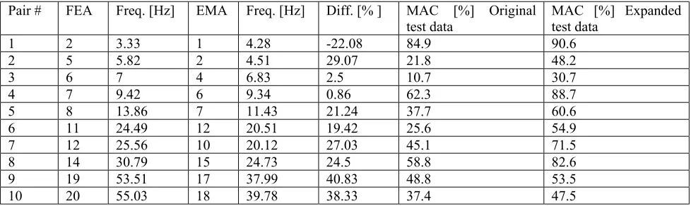
As a first task it was decided to evaluate how good the previously updated FE model was compared to test data obtained from measurements made with different BC, i.e. when piping has been insulated and filled with hot water (Case 3). In the ideal situation, there would only be some systematic shift in natural frequencies, which could easily be corrected by re-scaling the system matrices. There are several tools that can be used to sort out the experimental and analytical mode shapes that correlate best and to evaluate the quality of the FE model. The most commonly used tools are MAC and the EigenVector Orthogonality criterion (EVO). These are also often referred to as global shape correlation functions, because they only give an indication of the correlation level (similarity) of two different mode shape vectors. Here the MAC values and matrix are used to evaluate correlation levels and to construct mode pair tables between the updated FE model and experimental results in case of changed BC. The resulting mode pair table is shown in Table 5.

These results indicate that this FE model, which was updated according to Case 1 requirements, can be used as a base model for further updating to obtain an FE model matching Case 3 requirements. In general, mode shape correlation is quite good in some cases but a change in BC has shifted the natural frequencies significantly. It should be noted that the experimental modal database is obtained from two different measurements made using different shaker locations, while the modal database used for updating in Case 1 was made using only one shaker location. This means that there is now probably more structural information available than in the earlier case.

Table 5. Mode pair table between previously updated FE model and experimental results from Case 3 measurement set-up.

Pair # FEA Freq. [Hz] EMA Freq. [Hz] Diff. [% ] MAC [%] Original

test data MAC [%] Expandedtest data

1 2 3.33 1 4.28 -22.08 84.9 90.6

2 5 5.82 2 4.51 29.07 21.8 48.2

3 6 7 4 6.83 2.5 10.7 30.7

4 7 9.42 6 9.34 0.86 62.3 88.7

5 8 13.86 7 11.43 21.24 37.7 60.6

6 11 24.49 12 20.51 19.42 25.6 54.9

7 12 25.56 10 20.12 27.03 45.1 71.5

8 14 30.79 15 24.73 24.5 58.8 82.6

9 19 53.51 17 37.99 40.83 48.8 53.5

10 20 55.03 18 39.78 38.33 37.4 47.5

In order to perform an EVO check without system matrices or expansion of experimental modes, so-called pseudo-orthogonality check (POC) formulation [6] needs to be used. The evaluation of the mass POC is based on the following equality:

{ }

[ ]

{ } { } { }

a Ma e a e

ψ ψ ₌ ψ + ψ

(2)

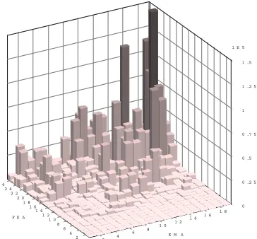
multiplied by the diagonal stiffness matrix. The mass POC matrix is shown in Fig. 3 and stiffness POC matrix in Fig. 4. The mass POC matrix indicates that the mass modelling is quite good for mode pairs FEA 2 and EMA 1, 7 and 6 and 14 and 15, and in general the highest terms are located close to the diagonal of the matrix. These were also the mode pairs with the highest MAC values in Table 5.

2 4 6 8 1 0 1 2 1 4 1 6 1 8

E M A 2

4 6 8 1 0 1 2 1 4 1 6 1 8 2 0 2 2 2 4 2 6

F E A

0 0 .2 0 .4 0 .6 0 .8 1 E V O M atrix (scaled P O C : M A S S )

Figure 3. Eigenvector orthogonality matrix with respect to mass. Note that values below 0.1 are filtered out.

The stiffness-related POC matrix does not look quite as good as the mass POC matrix, mainly due to high terms above the diagonal of the matrix. This matrix suggests that there are clearly some differences between stiffness modelling in the FE model and actual stiffness in the experimental model, and model updating efforts should perhaps concentrate from the start on stiffness related parameters.

2 4 6 8

1 0 1 2 1 4 1 6

1 8

E MA 2

4 6 8 1 0 1 2 1 4 1 6 1 8 2 0 2 2 2 4 2 6

F E A

1 E 5

0 0 .2 5 0 .5 0 .7 5 1 1 .2 5 1 .5

E V O M atrix (scaled P O C : S T IFFN E S S )

Error localisation

Local shape correlation analysis or so-called error localisation methods can be used for locating possible modelling discrepancies from mode pairs with unsatisfactory global correlation. These methods are also often referred to as spatial or DOF correlation analysis methods. The results from local shape correlation analysis serve as a guide for parameter selection for both sensitivity analysis and model updating. Here two different methods were used to localise areas with low correlation and possible modelling errors. First a co-ordinate orthogonality check (CORTHOG) was performed and the results of CORTHOG analysis were compared with those of modal force residues (MFR) analysis to identify more accurately those areas with possible modelling discrepancies.

The co-ordinate orthogonality check (CORTHOG) is used to identify how each DOF contributes to the overall orthogonality relationship between analytical and experimental modal vectors on a mass-weighted basis. The CORTHOG analysis evaluates the difference between obtained mass POC value and reference mass POC values at all DOF for all paired modes. A detailed description of the CORTHOG method can be found elsewhere [7]. Here the CORTHOG analysis was performed using a simple difference formulation, which retains the magnitude and direction of the error:

{ }

{ }

{ }

{

}

(

)

k

ij ik a jl e ik a j l a

k

SD CORTHOG= =

∑

where i an j denotes modes and k and l DOFs. j* indicates an analytical mode that is paired with experimental mode j. Higher CORTHOG values indicate areas with possible modelling discrepancies. This calculation could also be done using the left-hand side of the POC equality (Eq. 2) if there were a need to use an analytical mass matrix.

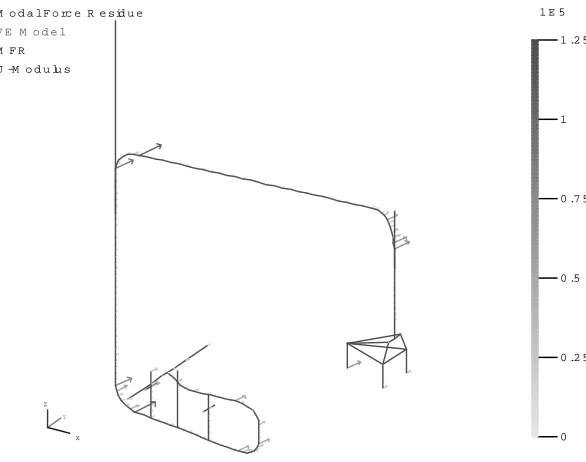
The modal force residues (MFR) are computed from the eigenvalue equation by substituting the analytical modes with expanded experimental modes [4]:

{

}

(

[ ] [ ]

)

{

}

where subscript e,exp refers to the expanded experimental modal vector and λ to analytical eigenvalues. Here the required expansion of experimental mode shapes was done using the so-called SEREP method with mass scaling. Higher MFR values indicate areas with possible modelling discrepancies.

The CORTHOG values in the case of mode pair 1 (Table 5) are shown in Fig. 5 summarised for all three directions (X, Y and Z). These values indicate that discrepancies between the experimental and analytical model in the case of mode pair 1 are mainly located at the lower part of the piping system, at the valves and at the points next to the pipe bends. This seemed to be the case also for mode pairs 4, 5 and 6. In the case of mode pairs 7 and 8 the main discrepancies seemed to be at the upper horizontal run. When the CORTHOG analysis was performed using the expanded test model, also the connection between the feed water pipeline and both the pump and the main feed water line then seemed to need further updating.

1E -2 3.5

3

2.5

2

1.5

1

0.5

0 U -M odulus

C O R T H O G P air 01 M A C 84.9

C oord. O rthogonality C heck (C O R T H O G )

FE M odel

Y

X Z

Figure 5. CORTHOG analysis results from mode pair 1.

1 E 5

1 .2 5

1

0 .7 5

0 .5

0 .2 5

0 M o d a l F o rc e R e sid u e

U -M o d u lu s M F R

F E M o d e l

Y

X Z

Figure 6. MFR analysis results in the case of experimental mode 1.

CONCLUSIONS

Model updating was performed successfully in the case of cold and non-insulated piping system, and the main focus during this update was on the ends of the FE model connection to the surrounding structures. Also, early in the numerical modelling the structural stiffness of the valves was modelled somewhat roughly, thus the stiffness of the elements modelling the valves was also modified.

During these correlation analyses it was discovered that discrepancies were higher in stiffness-related terms, and it might be advisable to concentrate on updating terms related to stiffness early in the model updating procedure. Further error localisation analyses also showed that the most problematic areas might be the lower part of the piping systems (very likely due to heavy valves) and pipe bends. Quite surprisingly the measurement points at the pump were not affected by changed BC, even if the connection between the feed water pipeline and the pump needs to be enhanced, as well as the connection between the feed water pipeline and main feed water pipeline at the other end of the piping.

ACKNOWLEDGEMENTS

This paper was prepared for a joint Finnish industry group as part of a project on Structural Operability and Plant Life Management (RKK). The project funding by the National Technology Agency (Tekes), Teollisuuden Voima Oy (TVO), Fortum Power and Heat Oy, Fortum Service Ltd., Fortum Nuclear Services Ltd., FEMdata Ltd., Neste Engineering Ltd., Fortum Oil and Gas Ltd.

REFERENCES

1. ABAQUS Theory Manual, Version 5.8. (1998). Hibbit, Karlsson & Sorensen Inc. RI.

2. Nurkkala, P., "Loviisa 1 syöttövesilinjan painepuolen RL61 putkiston moodianalyysi kolmella eri reunaehdolla elokuussa ja lokakuussa 2001", Fortum CMC, CMC-155. In Finnish.

3. Nurkkala, P., Luukkanen P., Saarenheimo A. and HaapaniemiH., "Model Updating through Measured Data in a Case of a Feed Water Pipe Line", to be published in Proc. of 17th Structural Mechanics in Reactor Technology, 2003. 4. FEMtools Theoretical Manual. Version 2.2.0. Dynamic Design Solutions N.V. (DDS). Leuven, Belgium, 2002. 5. O'Callahan, J., Avitabile, P. and Riemer, R., "System Equivalent Reduction Expansion Process (SEREP)", Proc. of 7th International Modal Analysis Conference, pp. 29-37, 1989.

6. Avitabile, P. and O'Callahan, J., "Mass and Stiffness Orthogonality Checks without a Mass or Stiffness Matrix", Proc. of 13th International Modal Analysis Conference, pp. 1515-1519, 1995.