ABSTRACT
RINKU MUKHERJEE. Post-Stall Prediction of Multiple-Lifting-Surface Con-figurations Using a Decambering Approach. (Under the direction of Dr. Ashok Gopalarathnam.)
Post-Stall Prediction of Multiple-Lifting-Surface
Configurations Using a Decambering Approach
by
Rinku Mukherjee
A dissertation submitted to the Graduate Faculty of North Carolina State University
in partial fulfillment of the requirements for the Degree of
Doctor of Philosophy
Aerospace Engineering
Raleigh, NC 2004
APPROVED BY:
Dr. Ashok Gopalarathnam Advisory Committee Chairman
Dr. Jack R. Edwards Dr. Fen Wu
Advisory Committee Member Advisory Committee Member
Dr. Zhilin Li
BIOGRAPHY
ACKNOWLEDGEMENTS
I extend my deepest gratitude to my advisor Dr. Ashok Gopalarathnam for his untiring support and encouragement without which this thesis would not be complete. He has taken personal efforts to provide guidance and both emotional and academic support during my time under him as a graduate student. Whether it was studying courses, writing conference papers, preparing for presentations, writing resumes or plain handling oneself professionally, he has always extended his undivided attention to every minute detail and helped me to become better than myself. His constant perseverance to do things better has been a great source of learning. In spite of his very busy schedules he found the time to give personal attention to every student in his continually growing research group. The greatest lesson that I have learnt from him as a researcher is to say “I do not know”. To acknowledge that one “does not know” and not fear the unknown can only lead to further and rigorous research and is perhaps one of the greatest qualities to possess as a researcher. Also, Dr. Gopalarathnam continually refers to research as “fun” and Cl-α plots as “beautiful” !!! That added so much colour to life and
made research lot more fun.
I am grateful to Dr. Jack R. Edwards, Dr. Fen Wu and Dr. Zhilin Li for being on my doctoral committee.
I thank Dr. Jack Edwards for his suggestions and invaluable advice in dealing with some of the very tricky problems in this research.
This research effort was supported under Grant NAG-1-01119 from the NASA Langley Research Center. This support and helpful discussions with the technical monitor, SungWan Kim, are gratefully acknowledged.
I thank my colleagues in my research group for making my graduate days less stressful.
Table of Contents
List of Figures . . . . ix
Nomenclature . . . xiii
Chapter 1 Introduction . . . . 1
1.1 Literature Study . . . 2
1.1.1 The Iterative Γ distribution Approach . . . 3
1.1.2 The α Correction Approach . . . 7
1.2 Current Approach . . . 9
Chapter 2 Illustration of the Decambering Concept for Flow Past an Airfoil . . . . 10
2.1 The Decambering Concept . . . 11
Chapter 3 Post-stall prediction of a finite wing . . . . 20
3.1 Decambering for a wing . . . 20
3.1.1 Vortex Lattice Method(VLM) . . . 21
3.1.2 Predicting the decambering along wing span . . . 21
3.2 The iteration procedure . . . 23
3.3 Multiple intersections in scheme 2 . . . 25
Chapter 4 Results . . . . 31
4.1.1 Rectangular Wing (AR=12) with the NACA 4415 Airfoil at
Re of 0.5 Million . . . 33
4.1.2 Effect of initial conditions on the iterations for Scheme 2 . 40 4.1.3 Rectangular Wing (AR=9) with the NACA 4415 Airfoil at Re of 0.5 Million . . . 41
4.1.4 Rectangular Wing (AR=6) with the NACA 4415 Airfoil at Re of 0.5 Million . . . 43
4.1.5 Rectangular Wing (AR=12) with the NACA 4415 Airfoil at Re of 0.75 Million . . . 45
4.1.6 Rectangular Wing (AR=9) with the NACA 4415 Airfoil at Re of 0.75 Million . . . 47
4.1.7 Rectangular Wing (AR=6) with the NACA 4415 Airfoil at Re of 0.75 Million . . . 49
4.1.8 Changes to the Lift Curve with Change to Aspect Ratio . 51 4.1.9 Summary . . . 56
4.2 Study of stall characteristics . . . 57
4.2.1 Stall Characteristics of a Part-Tapered Wing . . . 63
4.3 Wing-Tail Configuration . . . 65
4.4 Wing-Canard Configuration . . . 70
4.5 Spanwise Asymmetry in the Initial Conditions . . . 74
Chapter 5 Conclusions . . . . 82
Chapter 6 Future Work . . . . 86
Appendix A VLM3D . . . . 88
A.0.1 Subroutine readgeom . . . 88
A.0.3 Subroutine influence . . . 90
A.0.4 Subroutine readoper. . . 92
A.0.5 Subroutine dorhs . . . 92
A.0.6 Subroutine iteration . . . 92
List of Figures
2.1 Flow separation from an airfoil at a high angle of attack. . . 11
2.2 Schematic diagram of functions 1 and 2 (δ1 and δ2 are negative as shown) used to model effective decambering of an airfoil. . . 12
2.3 Cl and Cm of the NACA 0012 airfoil. . . 13
2.4 Cl and Cm using potential-flow with decambering. . . 14
2.5 The α s chosen to illustrate effectiveness of decambering. . . 15
2.6 Effectiveness of the decambering for α of 10 deg. . . 16
2.7 Effectiveness of the decambering for α of 16 deg. . . 17
2.8 Effectiveness of the decambering for α of 18 deg. . . 18
2.9 Flow chart of the iterative decambering approach in 2D flow. . . . 19
3.1 Vortex Lattice Method(only six lattices shown for clarity). . . 22
3.2 Flow chart of the iterative decambering approach for a wing(s). . 28
3.3 Illustration of the differences in the computation of the residuals using schemes 1 and 2. . . 29
3.4 Illustration of the different ways in which a trajectory line may intersect the airfoil Cl-α curve. . . 29
3.5 Flow chart for handling multiple intersections in Scheme 2 at a particular section on the wing(s). . . 30
4.1 Airfoil lift curves for the NACA 4415 airfoil from Naik and Ostowari17. 33 4.2 Planform of the rectangular wings (RHS shown) used in sec. 4.1. . 34
4.3 WingCL-α predicted using schemes 1 and 2 for a rectangular wing of aspect ratio 12, using a NACA 4415 airfoil at Reynolds number of 0.5 million. . . 34
4.4 SpanwiseCl distribution predicted for a rectangular wing of aspect ratio 12, using a NACA 4415 airfoil at Reynolds number of 0.5 million from scheme 1. . . 35
4.5 SpanwiseCl distribution predicted for a rectangular wing of aspect ratio 12, using a NACA 4415 airfoil at Reynolds number of 0.5 million from scheme 2. . . 36
4.7 Sawtooth in spanwise Cl distribution for a rectangular wing of
as-pect ratio 12, using a NACA 4415 airfoil at Reynolds number of 0.5 million from scheme 2. . . 39 4.8 Location of the upper and lower corners of the sawtooth region
shown in Fig. 4.7 on the NACA 4415 airfoil Cl-α curve. . . 40
4.9 WingCL-αpredicted for a rectangular wing of aspect ratio 12 using
a NACA 4415 airfoil at Reynolds number of 0.5 million for different starting values ofδ1. . . 41 4.10 Spanwise sectionCl predicted for a rectangular wing of aspect ratio
12 using a NACA 4415 airfoil at Reynolds number of 0.5 million for different starting values of δ1. . . 42 4.11 WingCL-α predicted using schemes 1 and 2 for a rectangular wing
of aspect ratio 9, using a NACA 4415 airfoil at Reynolds number of 0.5 million. . . 43 4.12 Spanwise Cl distribution predicted for a rectangular wing of
as-pect ratio 9, using a NACA 4415 airfoil at Reynolds number of 0.5 million from scheme 1. . . 44 4.13 Spanwise Cl distribution predicted for a rectangular wing of
as-pect ratio 9, using a NACA 4415 airfoil at Reynolds number of 0.5 million from scheme 2. . . 45 4.14 Wing CL-α predicted using scheme 2 for a rectangular wing of
aspect ratio 6, using a NACA 4415 airfoil at Reynolds number of 0.5 million. . . 46 4.15 Spanwise Cl distribution predicted for a rectangular wing of
as-pect ratio 6, using a NACA 4415 airfoil at Reynolds number of 0.5 million from scheme 2. . . 47 4.16 WingCL-α predicted using schemes 1 and 2 for a rectangular wing
of aspect ratio 12, using a NACA 4415 airfoil at Reynolds number of 0.75 million. . . 48 4.17 Spanwise Cl distribution predicted for a rectangular wing of aspect
ratio 12, using a NACA 4415 airfoil at Reynolds number of 0.75 million from scheme 1. . . 49 4.18 Spanwise Cl distribution predicted for a rectangular wing of aspect
ratio 12, using a NACA 4415 airfoil at Reynolds number of 0.75 million from scheme 2. . . 50 4.19 WingCL-α predicted using schemes 1 and 2 for a rectangular wing
of aspect ratio 9, using a NACA 4415 airfoil at Reynolds number of 0.75 million. . . 51 4.20 Spanwise Cl distribution predicted for a rectangular wing of aspect
ratio 9, using a NACA 4415 airfoil at Reynolds number of 0.75 million from scheme 1. . . 52 4.21 Spanwise Cl distribution predicted for a rectangular wing of aspect
4.22 Wing CL-α predicted using scheme 2 for a rectangular wing of
aspect ratio 6, using a NACA 4415 airfoil at Reynolds number
of 0.75 million. . . 54
4.23 Spanwise Cl distribution predicted for a rectangular wing of aspect ratio 6, using a NACA 4415 airfoil at Reynolds number of 0.75 million from scheme 2. . . 54
4.24 WingCL-α predicted from VLM3D for rectangular wings of aspect ratios 12, 9 and 6 using a NACA 4415 airfoil at Reynolds number of 0.5 million. . . 55
4.25 Wing CL-αpredicted from experiment for rectangular wings of as-pect ratios 12, 9 and 6 using a NACA 4415 airfoil at Reynolds number of 0.5 million. . . 55
4.26 Planform of the rectangular wing (RHS shown) used in sec. 4.2. . 57
4.27 Planform of the tapered wings (RHS shown) used in sec. 4.2. . . . 58
4.28 Airfoil lift curve used in sec. 4.2 – 4.5. . . 59
4.29 Wing CL-α for wings of different taper ratios, each of aspect ratio 10 using scheme 2. . . 60
4.30 Change in the spanwise section Cl distribution with taper at α of 10 deg using scheme 2. . . 60
4.31 Change in the spanwise section Cl distribution with taper at α of 17 deg using scheme 2. . . 61
4.32 Change in the spanwise section Cl distribution with taper at α of 18 deg using scheme 2. . . 61
4.33 Change in the spanwise section Cl distribution with taper at α of 24 deg using scheme 2. . . 62
4.34 Planform of the part-tapered wing (RHS shown). . . 62
4.35 Lift curves for the part-tapered wing. . . 63
4.36 Spanwise Cl distributions for the part-tapered wing. . . 64
4.37 Planform of the wing-tail configuration (RHS shown). . . 65
4.38 Lift curves for the wing-tail configuration. . . 66
4.39 Individual contributions of the wing and tail to the total lift of the wing-tail configuration. . . 67
4.40 Spanwise Cl distributions for the wing-tail configuration. . . 68
4.41 Pitching-moment curve for the wing-tail configuration. . . 69
4.42 Planform of the wing-canard configuration (RHS shown). . . 70
4.43 Lift curves of the wing-canard configuration. . . 71
4.44 Spanwise Cl distributions for the wing-canard configuration. . . . 72
4.45 Individual contributions of the wing and canard to the total lift of the wing-canard configuration. . . 73
4.46 Initial δ1 distribution along wing span. . . 74
4.47 Wing CL with an initial asymmetric distribution of δ1. . . 75
4.49 Spanwise section Cl with an initial asymmetric distribution of δ1
after 1 iteration. . . 77
4.50 Spanwise section Cl with an initial asymmetric distribution of δ1 after 100 iterations. . . 77
4.51 Final converged spanwise δ1 distributions. . . 78
4.52 Spanwise δ1 distributions after 1 iteration. . . 79
4.53 Spanwise δ1 distributions after 100 iterations. . . 79
4.54 Spanwise distributions of αef f after 1 iteration. . . 80
4.55 Spanwise distributions of αef f after 100 iterations. . . 80
4.56 Final converged spanwise distributions of αef f. . . 81
A.1 Unit normal to a lattice. . . 89
A.2 Horse-shoe vortex at the trailing edge. . . 91
Nomenclature
C damping factor
CL wing lift coefficient
Cl airfoil lift coefficient
Cm airfoil pitching moment coefficient about the quarter chord
c chord
F residual vector
f element of residual vector
i, j index of wing section
J Jacobian matrix
LLT lifting line theory
N number of wing sections
p perturbation to δ1 or δ2
VLM vortex lattice method
x2 chordwise start location of the second decambering function
β angle of yaw
Γ strength of bound vortex
δx vector containing the corrections to the Newton variables
δ1(x) first decambering function
δ2(x) second decambering function
θ2(x) angular coordinate corresponding to x2
Subscripts
1 scheme 1
2 scheme 2
max maximum
p perturbed value for a given step of the iteration
s starting value for a given step of the iteration
sec represents value for a wing section
t target value for a given step of the iteration
Chapter 1
Introduction
are also several additional isues that currently prevent the routine use of CFD for high-alpha predictions such as the time required for generating high-quality grids for each configuration. Thus the search for approximate approaches for stall and post-stall prediction of wings using known section data continues to be of interest. The approaches for extending the linear aerodynamic prediction methods to handle nonlinear and post-stall airfoil lift curves can be broadly classified into two kinds. In the first approach, a lift distribution is first assumed on the wing, and it is then iteratively corrected by determining the effective-α distribution using the nonlinear airfoil lift curve. In the second approach, the deviation of the airfoil nonlinear lift curve from the potential-flow linear lift curve is used to apply a correction to the local α at each section of the wing.
A literature study of the development of flow prediction methods over the years and brief descriptions of the two approaches follows.
1.1
Literature Study
2π per radian. With the success of LLT in the prediction of wing flows at low angles of attack, the attention soon turned to whether LLT could be modified for the analysis of wings where nonlinear lift-curve slopes for the airfoil sections can be taken into consideration. The studies in this regard can be widely divided into two categories as described below:
1.1.1
The Iterative
Γ
distribution Approach
Tani1 is believed to have developed the first successful technique in 1934 for han-dling nonlinear section lift-curve slopes in the LLT formulation. In his technique, a spanwise bound vorticity (Γ) distribution is first assumed; this distribution is used to compute the distribution of induced velocities and hence induced angles of attack and effective angles of attack along the lifting line. The distribution of the effective angles of attack is then used to look up the operating Cl of the local
section using the known nonlinearCl-αdata for the airfoil. A new Γ distribution
is then computed from the spanwise Cl distribution. The iteration is carried out
till the Γ distribution converges. This method worked well up to the onset of stall and was made popular by the NACA report of Sivells and Neely2 in 1947 that provided a detailed description of the method and implemented a tabular procedure for hand-calculation of the method for unswept wings with arbitrary planform and airfoil lift-curve slopes. This method was applied for analysis of wings up to the onset of stall, i.e. until a wing angle of attack at which some section on the wing has Cl equal to the local section Clmax. At higher angles of
attack where some sections on the wing may have a negative lift-curve slope, this successive-approximation approach appears to have failed.
post-stall angles of attack. According to Sears,4 von K´arm´an noticed that Prandtl’s lifting-line equation has non unique solutions for cases when the lift-curve slope becomes negative (i.e. when the α increases past the onset of stall). These non unique solutions include both symmetric and antisymmetric lift distributions even when both the geometry and onset flow are symmetric. Sears4 mentions that von K´arm´an further postulated that even in the conditions just past the onset of wing stall, when some sections of the wing may have positive lift-curve slopes (pre-stall condition) and other sections may have negative lift-curve slopes (post-(pre-stall condition), non unique and asymmetric lift distributions are possible. It occurred to von K´arm´an and Sears that the appearance of large and sometimes violent rolling moments past stall on symmetric wind-tunnel models at zero yaw may be explained by the possibility of asymmetric lift distributions at perfectly symmetric flight conditions.
stability of the two flows. Sears concludes by pointing out the need for further progress on the analysis of wings at near- and post-stall conditions.
Piszkin and Levinsky5 developed a nonlinear lifting line method based in part on the iterative method originally conceived by Tani.1 As described in Ref. 6, they were motivated by the need for a method that could predict, simulate, and alleviate adverse wing stalling characteristics such as wing drop, loss of roll control and roll control reversal at zero yaw. These characteristics were believed to be caused by the occurrence of asymmetric lift distributions on wings with stalled or partially-stalled flow.
The method of Piszkin and Levinsky utilizes a finite element, unsteady wake, incompressible flow theory that can be used for analysis at either zero or nonzero yaw. The model uses a single chordwise row of horseshoe vortices distributed along the span, with the bound vortex aligned with the local quarter-chord line. The boundary condition of zero normal flow is applied at the control point, which is the three-quarter-chord location for each horseshoe vortex. As a consequence of using a single chordwise horseshoe vortex, the method is restricted to wings of moderate to high aspect ratio. Although Levinsky refers to the method as a lifting-line method, the vortex model is more commonly referred to as a vortex lattice method (with a single chordwise row of horseshoe vortices) or a discrete-vortex Weissinger’s method. It must be mentioned that this method differs from Prandtl’s classical LLT in the implementation of the boundary condition.
number of iterations for convergence. Unlike in the traditional LLT, where the distribution of the effective section angles of attack is computed as part of the solution, with the vortex model that Piszkin and Levinsky used in their method, the distribution of the effective section angles of attack is not readily available. They have, however, bypassed this difficulty by defining the effective downwash angle at a section as α3D−α2D, where α3D is the downwash angle at the control
point resulting from the entire vortex system and α2D is the induced angle from
an infinite span bound vortex along thec/4 line with strength equal to that of the horseshoe vortex under consideration. From this downwash angle, they compute the effective angle of attack at every section of the wing. This formulation does not include the effects of sweep and dihedral for the effective angle of attack.6 Using their method, Piszkin and Levinsky found that multiple converged solutions are possible, including some that have saw-tooth type oscillations in the spanwise lift distributions. Because they were restricted to the use of 10 panels per side of the wing in their computer program, they were unable to determine whether these oscillations are present for more dense panel distributions. To avoid these oscillations, they used a switching logic that restarts the iteration procedure with an initial distribution having a zero induced α for any wing section found to be stalled.
a converged solution for a nonzero β as a starting point for the iteration. Like Sears, Levinsky6 also points out the need for a method of calculating the relative stability of the different possible solutions for the lift distribution at a given angle of attack. Finally, Levinsky6 points out the need for an unsteady nonlinear lifting surface theory that can handle low aspect ratio wings for fighters and other such configurations since until that point nonlinear methods were capable of handling only moderate to high aspect ratio wings. The Piszkin-Levinsky method has recently been used by Anderson7 for aircraft high-α stability analysis.
Four years after Levinsky’s publication, Anderson, Corda, and Van Wie8 pub-lished a nonlinear lifting-line theory that they applied to drooped leading-edge wings below and above stall. At that time, there was considerable interest in im-proving the stall-spin behavior of general aviation aircraft, and part-span drooped leading-edge wings were generating interest for their benign stall characteristics. Their article provides guidelines for the design of such wings and presents results for CL-α curves that extended to very high post-stall angles of attack close to 50
deg.
McCormick presents a similar, independently developed approach9 wherein the nonlinear lifting-line theory was used to examine the loss in roll damping for a wing near stall. In both Refs. 8 and 9, researchers reported that no asymmetric lift distributions for symmetric flight conditions are observed even when the iterations were started with asymmetric initial lift distribution. This observation differs from those of Sears and Levinsky.
1.1.2
The
α
Correction Approach
boundary-layer separation by iteratively reducing the angle of attack at each section of the wing. The reduction at any given wing section is determined by the difference between the potential flow solution and the viscousCl from the nonlinear section
Cl-α curve.
More recently, an approach similar to that reported in Ref. 10 was used by van Dam, Vander Kam and Paris11 for rapid estimation of CLmax and other high-lift characteristics for airplane configurations. In their method to estimate CLmax, at
least two airfoil data sets for the root and the tips are required for analysis. If there is significant variation in the spanwise wing geometry, then airfoil data for additional sections along the span are used. Using the sectional lift curves, the slope of the lift curve and zero lift angle of attack are calculated for each section along the wing span. Hence, the initial Cl distribution along span is calculated.
A complete sweep of angles of attack is then performed and at each angle of attack, an iterative procedure is employed to improve upon the initial spanwiseCl
distribution. The local effective angle of attack is calculated by adding a correction for viscous flow. If the difference between the viscous and linear potential section
Cl at a section is greater than a given tolerance then the section angle of attack
is corrected by a factor of the difference in the viscous and potential Cl to the lift
curve slope calculated earlier. Having made corrections to the distribution of α along the wing span, the modified Cl distribution is calculated. This process is
repeated till the difference in the viscous and potential Cl values at all spanwise
1.2
Current Approach
In the current research effort, a decambering approach (Scheme 1) was developed12 for predicting post-stall aerodynamic characteristics of wings using known section data. In this approach, the chordwise camber distribution at each section of the wing is reduced to account for the viscous effects at high angles of attack. This approach is somewhat similar to that developed in Ref. 10, but differs in its capability to use both the Cl and the Cm data for the section and in the
use of a two-variable function for the decambering. In addition, unlike all of the earlier methods, the current approach uses a multidimensional Newton iteration that accounts for the cross-coupling effects between the sections in predicting the decambering for each step in the iteration. This decambering approach was applied to the post-stall prediction of single wings in Ref. 12.
However, it was found that Scheme 1 worked for only some airfoil lift curves. Therefore, Scheme 2 was developed13 based on the same approach but differed in the way the residuals are computed. Scheme 2 is found to be more robust than Scheme 1 and works for several airfoil lift curves.
Chapter 2
Illustration of the Decambering
Concept for Flow Past an Airfoil
The overall objective of the current research is to arrive at a scheme for incorporat-ing the nonlinear section lift curves in wincorporat-ing analysis methods such as Liftincorporat-ing Line Theory (LLT), discrete-vortex Weissinger’s method and vortex lattice methods (VLM). For this purpose the wing span is assumed to consist of several sections and for each of these sections it is assumed that the two-dimensional data (Cl-α
and Cm-α) is available from either experimental or computational results.
Nonlinear lift curve slopes in wing analysis are incorporated by finding the effective angle of attack,αef f, and the corresponding effective reduction in camber
at each section of the wing. The effective reduction in camber or “decambering” is determined iteratively. The decambering at each section is modeled using a function of two variables.
in this chapter, its incorporation into the post-stall analysis of a three-dimensional wing is then discussed in Chapter3.
2.1
The Decambering Concept
This section illustrates the concept of decambering by using a simple example of a two-dimensional flow past a NACA 0012 airfoil. With increasing angle of attack, the boundary layer thickens on the upper surface and finally separates, as shown in Fig. 2.1. It is this flow separation that causes the viscous results for Cl
andCm to deviate from the predictions obtained using potential-flow theory. The
reason for the deviation can be related to the effective change in the airfoil camber distribution due to the boundary-layer separation. If the decambering is taken into consideration, then a potential-flow prediction for the decambered airfoil will closely match the viscous Cl and Cm for the high-α flow past the original airfoil
shape. This decambering idea served as the basis for the formulation of the current approach for the three-dimensional flow problem.
Figure 2.1: Flow separation from an airfoil at a high angle of attack.
While the camber reduction due to the flow separation can be determined from computational flows, no such detailed information is available from wind tunnel results that typically provide only theCl-α andCm-αcurves. This section
discusses the approach for determining an “equivalent” camber reduction from
Cl-α and Cm-α curves for an airfoil. More specifically, the effective decambering
for an α is computed using the deviations of the viscous Cl and Cm from the
x/c
0 1
δ1
(a)
Decambering function 1
x/c
0 1
δ2
(b)
x
2
Decambering function 2
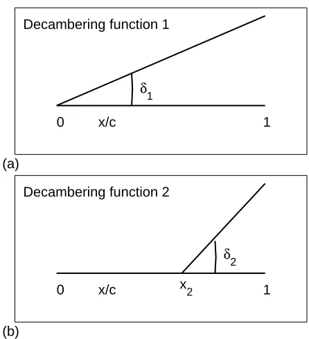
Figure 2.2: Schematic diagram of functions 1 and 2 (δ1 and δ2 are negative as shown) used to model effective decambering of an airfoil.
In the current method, the effective decambering for an airfoil is approximated using a function of two variables δ1 and δ2. The two linear functions shown in Fig. 2.2 are superposed to obtain the final decambering function. Two variables are used because the decambering is determined using two pieces of information: the Cl and Cm from the airfoil data for the α under consideration. This
ap-proximation will, of course, not match the actual viscous decambering, but the objective is to find an equivalent camber reduction to match the viscous Cl and
Cm for the α under consideration.
For the illustration of the decambering for two-dimensional flow over an airfoil, the following procedure is used:
1. Determine the viscous Cl andCm for theαunder consideration from
exper-imental or computational data for the airfoil.
2. Compute the corresponding potential-flow Cl and Cm using a lumped
α(deg) C
l
(a)
potential flow, original viscous flow, original
∆C
l
α(deg) Cm
(b)
potential flow, original viscous flow, original
∆C
m
Figure 2.3: Cl and Cm of the NACA 0012 airfoil.
approach of Katz and Plotkin,14 a thickness correction is applied to the Cl
by considering theCltimes the factor (1+0.77t/c) wheret/cis the maximum
thickness-to-chord ratio of the airfoil.
3. Compute the difference between the viscous and the potential-flow results: ∆Cl = (Cl)visc−(Cl)potential and ∆Cm = (Cm)visc−(Cm)potential.
These differences are shown schematically in Fig. 2.3 for an NACA 0012 airfoil analyzed using the XFOIL code.15
4. Use the differences ∆Cl and ∆Cm between the viscous and the
potential-flow Cl and Cm respectively to calculate the values of δ1 and δ2. Details of
this calculation follow:
The effects of changing δ1 and δ2 on the Cl and Cm for a given α can be
computed reasonably well using thin airfoil theory and a three-term Fourier series approximation for a flat plate with a flap deflection.14 The values of δ2 and δ1 in radians for a given ∆Cl and ∆Cm have been derived and are presented in Eqs. 2.1
α(deg) C
l
(a)
potential flow, original viscous flow, original potential flow, decambered
α(deg) Cm
(b)
potential flow, original viscous flow, original potential flow, decambered
Figure 2.4: Cl and Cm using potential-flow with decambering.
the start point for the second decambering function shown in Fig. 2.2(b) and can be expressed in terms of its x-location, denoted by x2, as shown in Eqn. 2.3. In the current work, x2/c is arbitrarily assumed to be 0.8, although any value from 0.5 to 0.9 typically works well. The overall approach used for this illustration is shown as a flow chart in Fig. 2.9.
δ2 = 1 ∆Cm 4 sin 2θ2− 12sinθ2
(2.1)
δ1 = ∆Cl−[2(π−2θπ2) + 2 sinθ2]δ2 (2.2)
θ2 =cos−1(1−2x2/c);x2/c= 0.8 (2.3)
To verify the effectiveness of the decambering approach, the values of δ1 and
δ2 were calculated for the viscous Cl-α and Cm-α data shown for the NACA 0012
−5 0 5 10 15 20 −1
−0.5 0 0.5 1 1.5 2
α(deg) C
l
A
B C
Figure 2.5: The α s chosen to illustrate effectiveness of decambering.
camberline for potential-flow analysis of the NACA 0012 airfoil using a lumped vortex method.14 Figure 2.4 shows for comparison the predicted potential-flow
Cl-α and Cm-α curves for the decambered airfoil with the viscous result from
XFOIL analysis. The agreement is seen to be very good, which confirmed that the two-variable decambering function can be used to model nonlinear lift as well as pitching moment curves for high angles of attack.
figures. Also observed is that the two-variable function used provides a reasonable approximation of the actual decambering of the airfoil.
(a) NACA 0012 airfoil with boundary layer atα of 10 deg.
0 0.1 0.2 0.3 0.4 0.5 0.6 0.7 0.8 0.9 1 −0.01
0 0.01 0.02 0.03 0.04 0.05 0.06 0.07 0.08
x/c
effective change in camber/c
decambering from present method
decambering from XFOIL
(b) Decambering function and XFOIL result.
(a) NACA 0012 airfoil with boundary layer atα of 16 deg.
0 0.1 0.2 0.3 0.4 0.5 0.6 0.7 0.8 0.9 1 −0.01
0 0.01 0.02 0.03 0.04 0.05 0.06 0.07 0.08
x/c
effective change in camber/c
decambering from present method
decambering from XFOIL
(b) Decambering function compared and result.
(a) NACA 0012 airfoil with boundary layer atα of 18 deg.
0 0.1 0.2 0.3 0.4 0.5 0.6 0.7 0.8 0.9 1 −0.01
0 0.01 0.02 0.03 0.04 0.05 0.06 0.07 0.08
x/c
effective change in camber/c
decambering from present method
decambering from XFOIL
(b) Decambering function compared and XFOIL result.
Yes
Assume starting decambering
G
1&
G
2Calculate residuals:
pot
l
visc
l
l
C
C
C
'
m
visc
m
pot
m
C
C
C
'
New
decambering:
G
1&
G
2Iteration
Converged
No
Residuals
within
Tolerance
Obtain viscous C
l& C
mfor original airfoil
(Available from experiment at operating
D
)
Calculate potential C
l& C
mfor decambered airfoil
Chapter 3
Post-stall prediction of a finite
wing
Using the overall methodology described in chapter 2, two schemes have been formulated for determining the post-stall solution of a finite wing. The primary difference between the two schemes is in the details of how the residuals, ∆Cl and
∆Cm, are computed at each section of the wing. The first scheme, introduced
in Ref. 12, was found to work well for certain airfoil lift curves, but failed to converge for several other airfoil lift-curves. This lack of robustness provided the impetus for developing the second scheme. The following sections explain the decambering approach for a wing, the overall iteration procedure used to implement the decambering approach, and the two schemes in detail.
3.1
Decambering for a wing
3.1.1
Vortex Lattice Method(VLM)
In a typical VLM, the lifting surface is divided into several spanwise and chord-wise lattices. Associated with each of these lattices is a ring vortex as shown in Fig. 3.1. The primary advantage of using ring vortex elements is that they can be easily implemented in a computer program. Also, the zero-normal-flow boundary condition is satisfied on the actual lifting surface which may have camber and different planform shapes. In the current work unsteady analysis is not done. Therefore, the wake behind the wing is not discretized and in order to satisfy the Kutta condition at the trailing edge the wake is replaced by a series of horse-shoe vortices. The leading segment of the vortex ring is placed on the lattice’s quar-ter chord line and the control point is at the cenquar-ter of the three-quarquar-ter chord line of the lattice. The zero-normal-flow boundary condition is satisfied at the control point of each lattice. A positive Γ is defined according to the right-hand rotation rule. Inthe current work, the VLM3D code was developed for analysis of multiple-lifting-surface configurations and the decambering approach was also implemented. A complete detailed description of the VLM3D code is provided in Appendix A.
3.1.2
Predicting the decambering along wing span
As explained earlier, the lifting surface is divided into several spanwise and chord-wise lattices. Each spanchord-wise section j (composed of a row of chord-wise lattices) has two variables, δ1j and δ2j, for defining the local decambered geometry at that
Wing T.E.
Trailing Vortices
x
Control Point Bound Vortices
Wing L.E. y
z Calculation Point of Lift
V∞
Figure 3.1: Vortex Lattice Method(only six lattices shown for clarity).
lifting surfaces. To account for these effects, a 2N-dimensional Newton iteration is used to predict the δ1 and δ2 at each of the N sections of all the wings so that the ∆Cl and ∆Cm at these sections approach zero as the iteration progresses. A
2N ×2N matrix equation as shown in Eqn. 3.1 has to be solved for each step of the Newton iteration.16 In this equation,Fis a 2N-dimensional vector containing the residuals of the functions fi to be zeroed, δx is the 2N-dimensional vector
containing the corrections required to the 2N variables xi to bring the vector F
closer to zero, andJis the 2N×2N Jacobian of the system containing the gradient information.
J·δx=−F (3.1)
J =
J
l1 Jl2
Jm1 Jm2
(3.2)
(Jl1)i,j =
∂∆Cli
∂δ1,j
= (Clp)i−(Cls)i [(δ1s)j +p]−(δ1s)j
(3.3)
(Jm1)i,j =
∂∆Cmi
∂δ1,j
= (Cmp)i −(Cms)i [(δ1s)j +p]−(δ1s)j
(3.4)
(Jl2)i,j =
∂∆Cli
∂δ2,j
= (Clp)i−(Cls)i [(δ2s)j +p]−(δ2s)j
(3.5)
(Jm2)i,j = ∂
∆Cmi
∂δ2,j
= (Cmp)i −(Cms)i [(δ2s)j +p]−(δ2s)j
(3.6)
For each step of the iteration, F and J are determined, and δx is computed using Eqn. 3.1. The corrections are then applied to the values of δ1 and δ2 for all the sections in an effort to bring the residuals closer to zero.
3.2
The iteration procedure
The iteration scheme can be summarized using the flow chart in Fig. 3.2, the illustration in Fig. 3.3 and the following procedure:
1. Assume starting values of the decambering defined by δ1 and δ2 for each section of the wing; for example, section j has starting values denoted by (δ1s)j and (δ2s)j;
the current step of the iteration and are denoted by (Cls)j and (Cms)j for
section j.
3. Compute the starting values of the local effective angles of attack of each section corresponding to the section Cl of that section; for example, the
local effective angle of attack of section j is obtained by setting (Cl)sec =
(Cls)j in Eqn. 3.7. Let this effective angle of attack be denoted by (αs)j.
Eqn. 3.7 assumes a section lift-curve slope of 2π per radian and accounts for the zero-lift angle of attack of the decambered section, which depends on the values of δ1 and δ2 and the α0l of the original airfoil camberline.
αef f =
(Cl)sec
2π −δ1−δ2[1−
θ2
π + sinθ2
π ] +α0l (3.7)
4. Residuals for Scheme 1: Compute the target Cl of each section; for
example, the target Cl of section j is given by (Clt,1)j (subscript 1 denotes
scheme 1), which is the Cl on the airfoil lift curve corresponding to (αs)j,
as shown in Fig. 3.3. Similarly, (Cmt,1)j, the target Cm, is the Cm on the
airfoil Cm-α curve corresponding to (αs)j. Hence, compute the residuals for
scheme 1 as (∆Cl,1)j = (Cls)j −(Clt,1)j and (∆Cm,1)j = (Cms)j −(Cmt,1)j.
5. Perturb δ1 at section j by adding a small perturbationp.
6. Compute the wing aerodynamic characteristics with the perturbed decam-bering using VLM3D; for example, the resultingCland Cm for sectionj are
denoted by (Clp)j and (Cmp)j. Hence, compute the jth column of Jl1 and
Jm1 using Eqns. 3.3 and 3.4.
7. Residuals for Scheme 2: Compute the local effective angle of attack of each section using the perturbed decambering; for example, the local effective angle of attack of sectionj is obtained by setting (Clsec) = (Clp)j in
the points [(αs)j,(Cls)j] and [(αp)j,(Clp)j] is called the “trajectory line,” as
it determines the linearized trajectory of how a point on the Cl-α curve
defined by the local sectionαef f and local section Cl moves with changes in
δ1. Therefore, in scheme 2, the targetCl, (Clt,2)j, of section j for example,
is the point of intersection between the trajectory line for section j and the airfoil lift curve, as illustrated in Fig. 3.3. The correspondingαis (αt,2)j and
(Cmt,2)j is the target Cm on the airfoil Cm-αcurve corresponding to (αt,2)j.
The residuals for scheme 2 are now computed as (∆Cl,2)j = (Cls)j−(Clt,2)j
and (∆Cm,2)j = (Cms)j−(Cmt,1)j.
8. Reset the value of δ1 at section j to (δ1s)j.
9. Cycle through steps 5–6 for all values of the section index j to compute all the columns of Jl1 and Jm1.
10. Repeat steps 5–9 now perturbing δ2 instead of δ1 to compute Jl2 and Jm2.
In this process, the computation of the residuals for scheme 2 in step 7 is ignored, as they have already been computed.
11. Using the Newton equation in Eqn. 3.1, compute the correction vector δx. Update the values of δ1s and δ2s by adding the correction vector δx multi-plied by a user-specified damping factorD(also referred to under-relaxation factor). In the current work, D has been set to 0.1.
This iteration process is carried out until all the residuals have converged to a specified tolerance. In the current work a tolerance of 0.001 has been used in all the examples.
3.3
Multiple intersections in scheme 2
Three possible ways in which the trajectory line may intersect the airfoil lift curve are illustrated in Fig. 3.4: (i) the trajectory line marked as L1 intersects the airfoil lift curve at a single pre-stall point, (ii) the trajectory line marked as L2 intersects the airfoil lift curve at multiple points and (iii) the trajectory line marked as L3 intersects the airfoil lift curve at a single point in the post-stall region. While there is no ambiguity in determining the values of the targetCl for lines L1
and L3, there are clearly three possible choices for the target Cl for line L2. This
illustration clearly demonstrates that it is possible to obtain multiple solutions for post-stall conditions; a fact, that was apparently first suggested by von K´arm´an (see Ref. 4) and has since been discussed by several researchers.3–6, 8, 9, 12 However, the approach in scheme 2 is novel because this scheme is believed to be the first one in which the possibility of multiple solutions for high angles of attack is brought to light right during the iteration process. Earlier approaches including scheme 1 were able to identify the existence of multiple solutions only as a result of obtaining multiple converged solutions with different initial conditions in the iteration procedure.
The existence of multiple intersections also presents a dilemma in choosing an appropriate targetCl from the possible multiple solutions. The following
pro-cedure was developed for making the choice during the intersection process. At each step of the iteration, each of the sections on all of the wings is examined to identify those with single intersections, as identified by points A and B in Fig. 3.4. The target Cl values for these sections are identified without ambiguity. Using
for the section is unstalled and the intersection point 3 is chosen if the logical switch for the section isstalled. This procedure is illustrated using a flow chart in Fig. 3.5.
Next, another logic is applied in which all the sections of the wings are scanned to identify sets of contiguous sections, all of which have multiple intersections and all of which are also tagged as unstalled. If any of these sets of contiguous sections are bound on both sides by sections tagged as stalled, then all the sections in this set are also tagged stalled. This logic removed any occurrence of unstalled regions with multiple-intersections sandwiched between two stalled regions.
Yes
Assume starting decambering,
G1
&
G2
at
several spanwise sections on the wing(s)
Compute C
l& C
mof each decambered section
(Numerical calculation using Vortex Lattice Method)
Obtain target C
l& C
mfrom airfoil data at each
decambered section (using one of two schemes)
(Available from experiment or 2D CFD)
Iteration
Converged
No
Compute local effective AOA,
D
sec
of each
decambered section
Residuals within Tolerance
Calculate residuals
'
C
l
&
'
C
m
using one
of two schemes
α
C
l
Cls C
lp
Clt,2
C
lt,1
δ δ + p
αs=α
t,1 αp αt,2
∆Cl,2
∆Cl,1
Trajectory line Airfoil
Figure 3.3: Illustration of the differences in the computation of the residuals using schemes 1 and 2.
α C
l
L1 A
L2 1
2 3
L3
B
Determine trajectory lines and intersections
Single intersection
stall
D
D
sec
(Trajectory line
L
1; Fig. 3.4)
stall
D
D
sec
!
(Trajectory line
L
3; Fig. 3.4)
x
Solution
B
(Fig. 3.4)
x
Reset
lpoststall
=True
Solution
1
(Fig. 3.4)
Multiple intersections
(Trajectory line L
2; Fig. 3.4)
Check value of
lpoststall
True
Solution
3
(Fig. 3.4)
x
Solution
A
(Fig. 3.4)
x
Reset
lpoststall
=False
Chapter 4
Results
The iterative decambering approach discussed in Chapter 3 has been implemented for the analysis of multiple-lifting-surface configurations in VLM3D, a custom VLM code. In this chapter, post-stall results from VLM3D are presented for several airfoil lift curves, different planform shapes and several lifting-surface con-figurations. The computation of the residual has been implemented using two schemes and the effectiveness of the two schemes are compared. The examples in this chapter are presented in five sections as follows:
1. Section 4.1: In this section, the examples have been used to compare the predicted results from the current method with experimental results from Naik and Ostowari.17 In their work,17experimentalCl-αdata for the NACA
4415 airfoil at Reynolds numbers of 0.5 million and 0.75 million are presented along with experimentalCL-αdata for finite constant-chord wings of several
2. Section 4.2: The objective of the second set of examples used in this section was to study the effect of planform shape on the stall characteristics of a wing. Tapered wings of different taper ratios are used to study where the wing first stalls and how the stall progresses along the span with increasing angle of attack.
3. Section 4.3: In this section, a wing-tail configuration is analyzed with the current method to demonstrate the capability of the current method to handle multiple-lifting-surface configurations. The effect of the wing stall on the aircraft pitching moment is shown to illustrate how the method can be used for providing information for the study of stability and control characteristics.
4. Section 4.4: A wing-canard configuration is used in this section to provide another example of an application to a multiple-lifting-surface configuration. This example illustrates how the canard stall behavior influences the wing lift distribution because of the downwash/upwash effects of the canard on the wing.
5. Section 4.5: In this section, an initial asymmetric distribution ofδ1is used for the iteration process to see if any asymmetries occur in the final converged
Cl distributions.
4.1
Experimental Validation
0 20 40 60 −0.5
0 0.5 1 1.5
α (deg) C
l
NACA 4415
Re = 0.5 x 10⁶ (exp) Re = 0.75 x 10⁶ (exp)
Figure 4.1: Airfoil lift curves for the NACA 4415 airfoil from Naik and Ostowari17.
then compared with the experimental CL-α curves for the corresponding wings
from the experimental data of Naik and Ostowari.17 The following sub-sections present the results for each case:
4.1.1
Rectangular Wing (AR=12) with the NACA 4415
Airfoil at Re of 0.5 Million
In this case, the airfoilCl-α curve is from the experimental data17 for the NACA
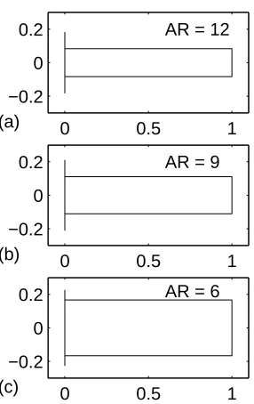
4415 airfoil at Re = 0.5 x 10⁶ (Fig. 4.1). A rectangular wing of aspect ratio 12 as shown in Fig. 4.2(a) is considered. Figure 4.3 shows the wing CL-α curves from
VLM3D using schemes 1 and 2. In the same figure, the airfoil Cl-α curve and
the wing CL-α curve from experiment17 are also shown for comparison. In both
0 0.5 1 −0.2
0
0.2 AR = 12
(a)
0 0.5 1
−0.2 0
0.2 AR = 9
(b)
0 0.5 1
−0.2 0
0.2 AR = 6
(c)
Figure 4.2: Planform of the rectangular wings (RHS shown) used in sec. 4.1.
0 20 40 60
−0.5 0 0.5 1 1.5
α(deg)
C l
and C
L
2D (experiment) 3D (experiment)
3D (VLM3D, Scheme 1) 3D (VLM3D, Scheme 2)
Figure 4.3: Wing CL-αpredicted using schemes 1 and 2 for a rectangular wing of
0 0.5 1 0
0.5 1 1.5
α = 18 deg
C
l
Clmax
0 0.5 1
0 0.5 1 1.5
α = 21 deg
0 0.5 1
0 0.5 1 1.5
α = 32 deg
Cl
0 0.5 1
0 0.5 1 1.5
α = 36 deg
Cl
0 0.5 1
0 0.5 1 1.5
α = 45 deg
C
l
y/(b/2)
0 0.5 1
0 0.5 1 1.5
α = 50 deg
y/(b/2)
Figure 4.4: Spanwise Cl distribution predicted for a rectangular wing of aspect
ratio 12, using a NACA 4415 airfoil at Reynolds number of 0.5 million from scheme 1.
As is seen from Fig. 4.3, the two schemes result in identical predictions for the wing CL for pre-stall angles of attack. For post-stall conditions, the results
of scheme 2 are closer to the experimental results. Figures 4.4 and 4.5 show the spanwiseCldistributions for angles of attack 18, 21, 32, 36, 45 and 50 degrees from
schemes 1 and 2 respectively. CLmax occurs at around α of 18 degrees. Experi-mental results for the spanwiseCl distributions were not available for comparison.
0 0.5 1 0
0.5 1 1.5
α = 18 deg
C
l
Clmax
0 0.5 1
0 0.5 1 1.5
α = 21 deg
0 0.5 1
0 0.5 1 1.5
α = 32 deg
Cl
0 0.5 1
0 0.5 1 1.5
α = 36 deg
Cl
0 0.5 1
0 0.5 1 1.5
α = 45 deg
C
l
y/(b/2)
0 0.5 1
0 0.5 1 1.5
α = 50 deg
y/(b/2)
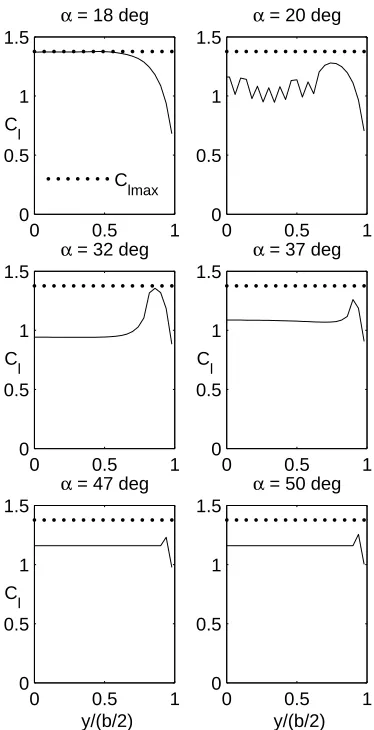
Figure 4.5: Spanwise Cl distribution predicted for a rectangular wing of aspect
ratio 12, using a NACA 4415 airfoil at Reynolds number of 0.5 million from scheme 2.
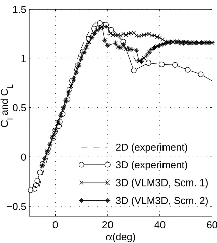
The wing CL from scheme 2 in Fig. 4.3 shows that as the α is increased to
18 deg, the CL continues to increase. At this condition the entire wing remains
unstalled as the local section Cl values are less than theCLmax of 1.39. This can
be confirmed by examining the spanwise sectionCl distribution from scheme 2 in
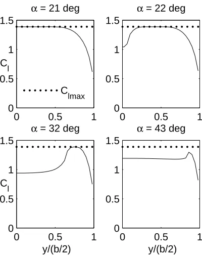
Fig. 4.5 forαof 18 deg. At 18 deg the inboard portion of the wing is close to stall. As theα is increased between 18 deg and 21 deg, a part of the inboard portion of the wing stalls and another part is close to stall as can be seen from the spanwise sectionCl distribution forαof 21 deg in Fig. 4.5. As the αis increased beyond 21
deg, the spanwise extent of the stalled portion increases. At 32 deg most of the wing has stalled and the outboard portion is close to stall as shown in Fig. 4.5. Between 32 deg and 44 deg the Cl on the stalled portion of the wing increases.
The wing CL therefore increases between 32 deg and 44 deg as shown in Fig. 4.3.
Beyond 44 deg, theCl on the wing does not increase anymore. In fact, it remains
almost constant at 1.2, as shown in Fig. 4.5 for αof 45 deg. At 50 deg, the entire wing has stalled as seen from the spanwise sectionCl distribution for αof 50 deg.
Therefore the wing CL decreases between 44 deg and 51 deg.
The wing CL-α from scheme 1 on the other hand does not show a marked
decrease when the α is increased between 18 and 32 deg as shown in Fig. 4.3. This can be explained by investigating the spanwise sectionCl distributions from
scheme 1 forα of 32, 36, 45 and 50 deg in Fig. 4.4. There is considerable sawtooth behavior and no large-scale stalling of the wing. Even at 50 deg there are several unstalled sections sandwiched between stalled sections. Hence, although the wing
CLdrops after 18 deg as some sections stall, it does not show any marked decrease
or a CL minimum.
0 200 400 600 800 1000 1.13
1.14 1.15 1.16 1.17 1.18
α = 27 deg
number of iterations C
L
Figure 4.6: Wing CL variation with number of iterations for a rectangular wing
of aspect ratio 12, using a NACA 4415 airfoil at Reynolds number of 0.5 million from scheme 2.
example, the iterations did not converge at α of 27 deg and Fig. 4.6 shows the variation of the wingCL with number of iterations for αof 27 deg. It is seen that
the convergence plot for the wingCL exhibits an undamped periodic behavior and
minimum values but does not converge.
0 0.2 0.4 0.6 0.8 1 0.8
0.9 1 1.1 1.2 1.3 1.4 1.5
y/(b/2) C
l
α = 21 deg
Unstalled section Stalled section
Figure 4.7: Sawtooth in spanwiseCl distribution for a rectangular wing of aspect
ratio 12, using a NACA 4415 airfoil at Reynolds number of 0.5 million from scheme 2.
Also, for α of 21 deg, oscillations were observed in the spanwise section Cl
distribution as shown in Fig. 4.5. This sawtooth region atαof 21 deg is examined closely in Fig. 4.7 and it illustrates that the sawtooth occurs because of unstalled sections sandwiched between stalled sections. Such oscillations were observed for some angles of attack in the sequence, some of which have final converged solutions. Figure 4.8 shows the section Cl plotted against the section effective
angle of attack on the airfoilCl-αcurve for the points corresponding to the upper
and lower corners of the sawtooth region. It is seen that the upper corners of the sawtooth region (marked by “*” in Figs. 4.7 and 4.8) have converged to the unstalled region of the airfoilCl-αcurve as shown in Fig. 4.8 and the lower corners
0 20 40 60 −0.5
0 0.5 1 1.5
α(deg) Cl
2D (experiment) Stalled sections Unstalled sections
α = 21 deg
Figure 4.8: Location of the upper and lower corners of the sawtooth region shown in Fig. 4.7 on the NACA 4415 airfoil Cl-α curve.
lines for the upper corner points intersect the airfoil Cl-α curve at only a single
point, the post-stall logic was unable to remove such oscillations.
4.1.2
Effect of initial conditions on the iterations for
Scheme 2
It must be mentioned that for a majority of the cases, Scheme 2 is successful in converging to realistic solutions with no “sawtooth behavior”. It is only for a few conditions that the converged solution has a sawtooth behavior (e.g. α = 21 deg in Fig. 4.5) or the solution does not converge due to an undamped periodic con-vergence pattern as shown in Fig. 4.6. Figure 4.9 shows the wing CL-α predicted
using scheme 2 for two different starting conditions for the Newton Iteration: (a)
δ1 =−40 deg for all sections at each α and (b) δ1 = 0 deg for all sections at each
0 20 40 60 −0.5
0 0.5 1 1.5
α(deg)
C l
and C
L
2D (experiment) 3D(VLM3D, δ
1=−40 deg at each α)
3D(VLM3D, δ
1=0 deg at each α)
Figure 4.9: WingCL-αpredicted for a rectangular wing of aspect ratio 12 using a
NACA 4415 airfoil at Reynolds number of 0.5 million for different starting values of δ1.
deg. The results clearly illustrate that multiple solutions are possible for post-stall conditions. Furthermore, the results do not provide any clear guidelines as to which is the correct solution. It can however be said that the different schemes and starting assumptions predict the wingCLfor a given post-stall angle of attack
within a small scatter band. The scatter shown confirms the possibility of multiple solutions at post-stall angles of attack pointed out by other researchers3–6, 8, 9, 12 and the sensitivity of post-stall solutions to initial conditions as well as schemes used for the Newton iteration.
4.1.3
Rectangular Wing (AR=9) with the NACA 4415
Airfoil at Re of 0.5 Million
For this case also, the airfoil Cl-α curve is from experiment and is as shown in
0 0.5 1 0
0.5 1 1.5
α = 18 deg
Cl
δ1 = 0 deg
y/(b/2)
0 0.5 1
0 0.5 1 1.5
α = 18 deg
δ1 = −40 deg
y/(b/2)
Figure 4.10: Spanwise section Cl predicted for a rectangular wing of aspect ratio
12 using a NACA 4415 airfoil at Reynolds number of 0.5 million for different starting values of δ1.
Fig. 4.2, is studied. Figure 4.11 shows the wing CL-α curves from VLM3D using
schemes 1 and 2. In the same figure the airfoil Cl-α curve and the wing CL-α
curve from experiment17 are also shown for comparison. In both schemes, the starting values of δ1 and δ2 were taken from the converged results of the previous
α. For the first α of the sequence, δ1 was set to −40 deg and δ2 was set to 0 deg for both schemes. A sequence of angles of attack from −5 to 60 deg was used and a few angles of attack did not converge for scheme 2. In Fig. 4.11 the wingCL for
only the converged angles of attack are plotted for scheme 2.
It is evident again from Fig. 4.11 that in comparing the results of the two schemes with the experimental data, scheme 2 gives a better comparison with experiment. Figs. 4.12 and 4.13 show the spanwise section Cl distribution for
α of 20, 21, 32, 42, 44 and 50 degrees from scheme 1 and scheme 2 respectively.
CLmaxoccurs at aroundαof 20 degrees. Experimental results for the spanwise Cl
distributions were not available for comparison. As seen from the results of scheme 1 in Fig. 4.12, there is substantial sawtooth behavior in the spanwise section Cl
0 20 40 60 −0.5
0 0.5 1 1.5
α(deg)
C l
and C
L
2D (experiment) 3D (experiment)
3D (VLM3D, Scheme 1) 3D (VLM3D, Scheme 2)
Figure 4.11: Wing CL-α predicted using schemes 1 and 2 for a rectangular wing
of aspect ratio 9, using a NACA 4415 airfoil at Reynolds number of 0.5 million.
within a tolerance of 0.001 in ∆Cl and ∆Cm.
4.1.4
Rectangular Wing (AR=6) with the NACA 4415
Airfoil at Re of 0.5 Million
In this case also, the airfoil Cl-α curve is from experiment and is as shown in
Fig. 4.1 for Re = 0.5 x 10⁶. A rectangular wing of aspect ratio 6, as shown in Fig. 4.2, is studied. Figure 4.14 shows the wing CL-α curve from VLM3D using
scheme 2. In the same figure the airfoil Cl-α curve and the wing CL-α curve
0 0.5 1 0
0.5 1 1.5
α = 20 deg
C
l
Clmax
0 0.5 1
0 0.5 1 1.5
α = 21 deg
0 0.5 1
0 0.5 1 1.5
α = 32 deg
Cl
0 0.5 1
0 0.5 1 1.5
α = 42 deg
Cl
0 0.5 1
0 0.5 1 1.5
α = 44 deg
C
l
y/(b/2)
0 0.5 1
0 0.5 1 1.5
α = 50 deg
y/(b/2)
Figure 4.12: Spanwise Cl distribution predicted for a rectangular wing of aspect
ratio 9, using a NACA 4415 airfoil at Reynolds number of 0.5 million from scheme 1.
attack are plotted for scheme 2.
Fig. 4.15 shows the spanwise section Cl distribution for α of 21, 22, 32, and
0 0.5 1 0
0.5 1 1.5
α = 20 deg
C
l
Clmax
0 0.5 1
0 0.5 1 1.5
α = 21 deg
0 0.5 1
0 0.5 1 1.5
α = 32 deg
Cl
0 0.5 1
0 0.5 1 1.5
α = 42 deg
Cl
0 0.5 1
0 0.5 1 1.5
α = 44 deg
C
l
y/(b/2)
0 0.5 1
0 0.5 1 1.5
α = 50 deg
y/(b/2)
Figure 4.13: Spanwise Cl distribution predicted for a rectangular wing of aspect
ratio 9, using a NACA 4415 airfoil at Reynolds number of 0.5 million from scheme 2.
4.1.5
Rectangular Wing (AR=12) with the NACA 4415
Airfoil at Re of 0.75 Million
In this case, the airfoil Cl-α curve is from experiment and is as shown in Fig. 4.1
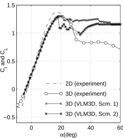
for Re = 0.75 x 10⁶. A rectangular wing of aspect ratio 12, as shown in Fig. 4.2, is studied. Figure 4.16 shows the wing CL-α curves from VLM3D using schemes
1 and 2. In the same figure the airfoil Cl-α curve and the wing CL-α curve from
0 20 40 60 −0.5
0 0.5 1 1.5
α(deg)
C l
and C
L
2D (experiment) 3D (experiment) 3D (VLM3D, Scm.2)
Figure 4.14: WingCL-αpredicted using scheme 2 for a rectangular wing of aspect
ratio 6, using a NACA 4415 airfoil at Reynolds number of 0.5 million.
first α of the sequence, δ1 was set to −40 deg and δ2 was set to 0 deg for both schemes. A sequence of angles of attack from −5 to 60 deg was used and a few angles of attack did not converge for scheme 2. In Fig. 4.16, the wingCL of only
the converged angles of attack are plotted for scheme 2.
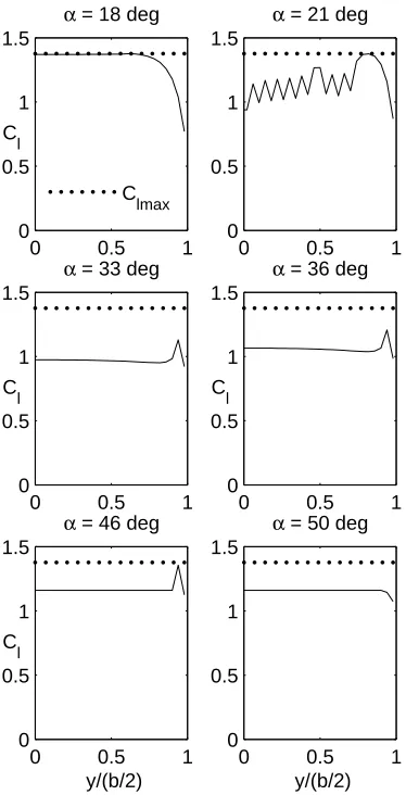
As observed before, it can be seen from Fig. 4.16 that scheme 2 gives a better comparison with experiment. Figs. 4.17 and 4.18 show the spanwise section Cl
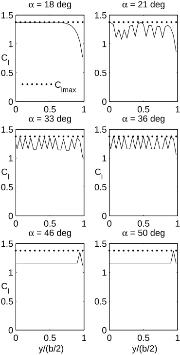
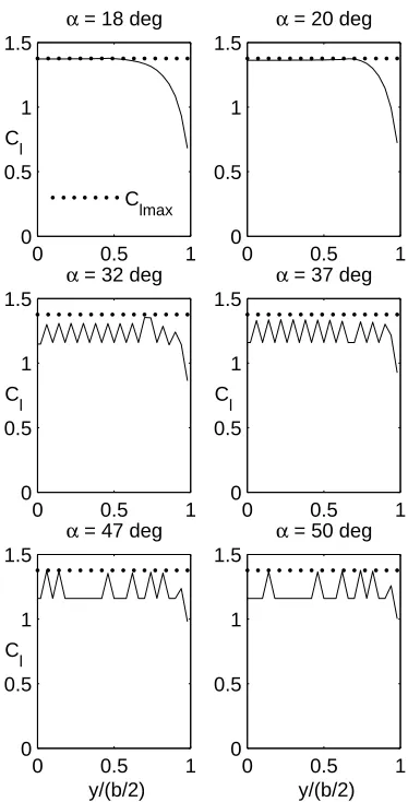
distribution for α of 18, 21, 33, 36, 46 and 50 degrees from scheme 1 and scheme 2 respectively. CLmax occurs at aroundα of 18 degrees. Experimental results for the spanwise Cl distributions were not available for comparison. As seen from
the results of scheme 1 in Fig. 4.17, there is substantial sawtooth behavior in the spanwise section Cl distributions. On the other hand, the results from scheme 2
0 0.5 1 0
0.5 1 1.5
α = 21 deg
C
l
Clmax
0 0.5 1
0 0.5 1 1.5
α = 22 deg
0 0.5 1
0 0.5 1 1.5
α = 32 deg
C
l
y/(b/2)
0 0.5 1
0 0.5 1 1.5
α = 43 deg
y/(b/2)
Figure 4.15: Spanwise Cl distribution predicted for a rectangular wing of aspect
ratio 6, using a NACA 4415 airfoil at Reynolds number of 0.5 million from scheme 2.
for aspect ratio of 12.
4.1.6
Rectangular Wing (AR=9) with the NACA 4415
Airfoil at Re of 0.75 Million
In this case the airfoil Cl-α curve is from experiment and is as shown in Fig. 4.1
for Re = 0.75 x 10⁶. A rectangular wing of aspect ratio 9 as shown in Fig. 4.2 is studied. Figure 4.19 shows the wing CL-α curves from VLM3D using schemes
1 and 2. In the same figure the airfoil Cl-α curve and the wing CL-α curve from