Modeling and Computing for Layered Pavements Under Vehicle Loading

(1)

ABSTRACT

XU, QINGXIA. Modeling and Computing for Layered Pavements under Vehicle Loading. (Under the direction of Dr. M. Shamimur Rahman and Dr. Akhtarhusein A. Tayebali)

(2)

MODELING AND COMPUTING FOR LAYERED PAVEMENTS UNDER VEHICLE LOADING

by QINGXIA XU

A dissertation submitted to the Graduate Faculty of North Carolina State University

in partial fulfillment of the requirements for the Degree of

Doctor of Philosophy

CIVIL ENGINEERING Raleigh

2004

APPROVED BY:

M. S. Rahman A. A. Tayebali

(Chair of Advisory Committee) (Co-chair of Advisory Committee)

(3)

BIOGRAPHY

Qingxia Xu was born in Wuhan, China, 1974. She received her Bachelor degree

in Hydrogeology and Engineering Geology from Ocean University of Qingdao, Qingdao,

China, in 1995. She received her Masters of Science degree in Geotechnical Engineering

from Tongji University, Shanghai, China, in 1998. In 2000, Qingxia came to North

Carolina State University, Raleigh, North Carolina, USA to study for her Ph.D. in

(4)

ACKNOWLEDGEMENTS

First and foremost, I would like to give my sincere thanks to my advisor, Dr. M.

Shamimur Rahman, for providing me such a wonderful opportunity to study at NCSU

and giving me numerous valuable guidance and inspiration for my research.

I would like to thank Dr. Akhtarhusein A.Tayebali, my co-advisor, for his time,

knowledge and providing me the testing data of his research project.

Many thanks go to Professor J. C. Small for providing me the detailed derivation

of the finite layer theory, Professor H. H. Winter for offering me the software IRIS for

the evaluation of viscoelastic model parameters, Professor Z. L. Feng for his help and

support.

Thanks to my committee members, Dr. Roy Borden, Dr. Mohammed Gabr and Dr.

N. Paul Khosla. I appreciate your time and effort.

Thanks to Dr. Moreshwar B. Kulkarni for his time and help.

Special thanks to my husband, Yuanxiong Huang, for his support, help and

(5)

LIST OF TABLES

TABLE 2.1 BRAKING EFFECT AND FORCE TRANSFERRED TO THE PAVEMENT DUE TO SKID

RESISTANCE [13] ... 34

TABLE 2.2 SPS-9APROJECT 370900,HIGHWAY US-1NORTHBOUND,SANFORD,NC,

PAVEMENT STRUCTURE –NEW CONSTRUCTION... 35

TABLE 2.3 ASPHALT BINDER AND AGGREGATES USED IN THE PAVEMENT STRUCTURE.... 35

TABLE 2.4 AGGREGATE GRADATIONS... 36

TABLE 2.5 SHEAR STRENGTHS UNDER VARIOUS NORMAL STRESSES WITH SHEARING RATE

0.625MM/MIN AT 20ºC... 36

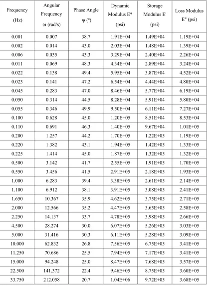
TABLE 3.1 RAW DATA FOR AN ASPHALT CONCRETE BEAM SUBJECTED TO AXIAL

FREQUENCY TEST AT TEMPERATURE 20ºC ... 99

TABLE 3.2 PARAMETERS OF THE GENERALIZED MAXWELL MODEL FOR AN AC BEAM SAMPLE... 110

(9)

LIST OF FIGURES

FIGURE 2.1 MODEL OF LAYERED PAVEMENT SYSTEM... 37

FIGURE 2.2 ILLUSTRATION OF NORMAL STRESS AND SHEAR STRESS AT THE INTERFACE. 37 FIGURE 2.3 CONTINUITY CONDITION AT THE INTERFACE... 38

FIGURE 2.4 INTEGRATION SCHEME... 38

FIGURE 2.5 FLOW CHART FOR SOLUTION PROCEDURE... 39

FIGURE 2.6 AXIS TRANSFORMATION... 39

FIGURE 2.7 NORMAL STRESS DISTRIBUTIONS ALONG THE CENTERLINE FOR SINGLE LAYER ... 40

FIGURE 2.8 NORMAL STRESS DISTRIBUTIONS ALONG THE CENTERLINE FOR A THREE -LAYERED SYSTEM... 40

FIGURE 2.9 DISTRIBUTION OF STRESSES AT SURFACE Z/A =1 FOR A HALF SPACE... 41

FIGURE 2.10 INTERFACE SHEAR STRESS FOR A TWO-LAYERED SYSTEM SUBJECTED TO CIRCULAR SHEAR LOAD ON THE SURFACE... 41

FIGURE 2.11 TYPICAL SLIPPAGE FAILURE [12]... 42

FIGURE 2.12 PAVEMENT STRUCTURE USED IN THE ANALYSIS... 42

FIGURE 2.13 DISTRIBUTION OF SHEAR STRESS τXZ AT THE INTERFACE (Z=1.5", X=0) ALONG Y-AXIS (VP: VERTICAL PRESSURE,HP: HORIZONTAL PRESSURE) ... 43

FIGURE 2.14 DISTRIBUTION OF SHEAR STRESS τXZ AT THE INTERFACE ALONG X-AXIS (Z=1.5", Y=0)(VP: VERTICAL PRESSURE,HP: HORIZONTAL PRESSURE) .... 43

FIGURE 2.15 3-D PRESENTATION OF SHEAR STRESS RESULTANT AT THE INTERFACE (Z=1.5") UNDER 100PSI VERTICAL PRESSURE AND 68PSI HORIZONTAL PRESSURE... 44

(10)

FIGURE 2.17 DISTRIBUTION OF SHEAR STRESS AT THE INTERFACE (Z =1.5″) FOR VARIOUS THICKNESS OF THE FIRST LAYER UNDER 100PSI VERTICAL AND 68PSI

HORIZONTAL PRESSURE... 45

FIGURE 2.18 PICTURE OF TWO TYPES OF SAMPLE... 45

FIGURE 2.19 TYPICAL INTERFACE FAILURE (A)... 46

FIGURE 2.20 TYPICAL INTERFACE FAILURE (B) ... 46

FIGURE 2.21 TYPICAL INTERFACE FAILURE (C) ... 47

FIGURE 2.22 TYPICAL SHEAR STRESS VERSUS DISPLACEMENT CURVE FOR STRAIN CONTROLLED SHEAR TESTING... 47

FIGURE 2.23 RELATIONSHIP BETWEEN NORMAL STRESS AND SHEAR STRENGTH WITH SHEARING RATE 0.625MM/MIN AT 20ºC FOR THE SP12.5 OVER SP19 SAMPLES... 48

FIGURE 2.24 RELATIONSHIP BETWEEN NORMAL STRESS AND SHEAR STRENGTH WITH SHEARING RATE 0.625MM/MIN AT 20ºC FOR THE SP19 OVER SP37.5 SAMPLES... 48

FIGURE 3.1 SOLUTION FLOW CHART FOR VISCO-ELASTIC MATERIAL ANALYSIS... 89

FIGURE 3.2 VISCOELASTIC BAR... 90

FIGURE 3.3 CREEP... 90

FIGURE 3.4 STRESS RELAXATION... 90

FIGURE 3.5 A LINEAR SPRING... 91

FIGURE 3.6 ANEWTONIAN DASHPOT... 91

FIGURE 3.7 THE MAXWELL MODEL... 91

FIGURE 3.8 THE KELVIN MODEL... 91

FIGURE 3.9 THE GENERALIZED MAXWELL MODEL... 92

FIGURE 3.10 THE GENERALIZED KELVIN MODEL... 92

FIGURE 3.11 CONVOLUTION INTEGRAL... 92

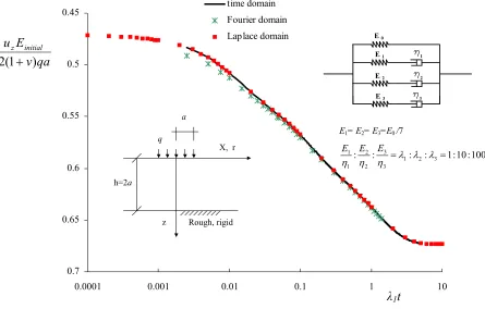
FIGURE 3.12 TIME–DEFLECTION RELATIONSHIP FOR CONSTANT CIRCULAR LOADING ON SINGLE VISCOELASTIC LAYER... 93

(11)

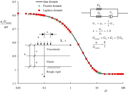
FIGURE 3.14 TIME–DEFLECTION RELATIONSHIP FOR CONSTANT CIRCULAR LOADING ON

TWO-LAYERED VISCOELASTIC-ELASTIC SYSTEM. ... 95

FIGURE 3.15 (A)STRESSES AND (B) STRAINS ON CENTERLINE BENEATH THE CIRCULAR LOADING FOR A TWO-LAYERED SYSTEM... 96

FIGURE 3.16 HAVERSINE LOADING OF SIN KT... 97

FIGURE 3.17 SEVEN PARAMETER GENERALIZED KELVIN MODEL... 97

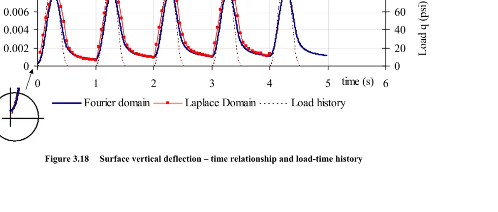
FIGURE 3.18 SURFACE VERTICAL DEFLECTION – TIME RELATIONSHIP AND LOAD-TIME HISTORY... 98

FIGURE 3.19 STORAGE MODULUS E' BY TESTING AND FITTING CURVE... 100

FIGURE 3.20 LOSS MODULUS E" BY TESTING AND FITTING CURVE... 100

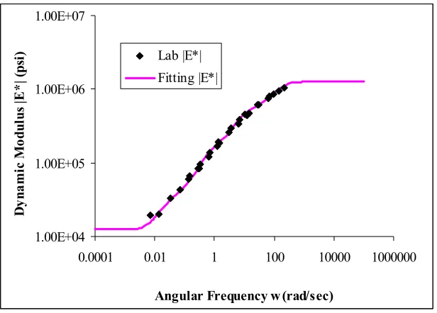
FIGURE 3.21 MASTER CURVE OF DYNAMIC MODULUS |E*| BY TESTING AND CURVE -FITTING... 101

FIGURE 3.22 THREE-LAYER PAVEMENT SYSTEM... 101

FIGURE 3.23 STRESS-ZZ DISTRIBUTION BELOW THE TIRE CENTER... 102

FIGURE 3.24 STRESS-YY DISTRIBUTION BELOW THE TIRE CENTER... 102

FIGURE 3.25 STRESS-XX DISTRIBUTION BELOW THE TIRE CENTER... 103

FIGURE 3.26 STRESS-XZ DISTRIBUTION BELOW THE TIRE CENTER... 103

FIGURE 3.27 STRESS-YZ DISTRIBUTION BELOW THE TIRE CENTER... 104

FIGURE 3.28 STRAIN-ZZ DISTRIBUTION BELOW THE TIRE CENTER... 104

FIGURE 3.29 STRAIN-YY DISTRIBUTION BELOW THE TIRE CENTER... 105

FIGURE 3.30 STRAIN-XX DISTRIBUTION BELOW THE TIRE CENTER... 105

FIGURE 3.31 STRESS-ZZ DISTRIBUTION BELOW THE TIRE EDGE POINT (0,3.785)... 106

FIGURE 3.32 STRESS-YY DISTRIBUTION BELOW THE TIRE EDGE POINT (0,3.785)... 106

FIGURE 3.33 STRESS-XX DISTRIBUTION BELOW THE TIRE EDGE POINT (0,3.785)... 107

FIGURE 3.34 STRESS-XZ DISTRIBUTION BELOW THE TIRE EDGE POINT (0,3.785) ... 107

FIGURE 3.35 STRESS-YZ DISTRIBUTION BELOW THE TIRE EDGE POINT (0,3.785) ... 108

FIGURE 3.36 STRAIN-ZZ DISTRIBUTION BELOW THE TIRE EDGE POINT (0,3.785) ... 108

FIGURE 3.37 STRAIN-YY DISTRIBUTION BELOW THE TIRE EDGE POINT (0,3.785)... 109

FIGURE 3.38 STRAIN-XX DISTRIBUTION BELOW THE TIRE EDGE POINT (0,3.785)... 109

(12)

FIGURE 4.1 STRAIN DECOMPOSITION FROM CREEP AND RECOVERY TEST (BY UZAN [3])...

... 128

FIGURE 4.2 SCHEMATIC REPRESENTATION OF NON-LINEAR VISCOELASTIC MODEL WITH SLIDER[6]... 128

FIGURE 4.3 STRAIN VS. TIME RESPONSE FOR THE CREEP AND RECOVERY TEST AT 35ºC(BY SCHWARTZ [9])... 129

FIGURE 4.4 BEST FIT MODEL IN LOG-LOG SPACE.(BY SCHWARTZ [9]) ... 129

FIGURE 4.5 ELASTO-PLASTIC MODEL... 130

FIGURE 4.6 ELASTO-VISCO-PLASTIC MODEL... 130

FIGURE 4.7 SCHEMATIC RUTTING ANALYSIS MODEL... 131

FIGURE 4.8 SCHEMATIC MODEL FOR PAVEMENT RUTTING ANALYSIS... 131

FIGURE 4.9 ELASTIC LINEAR STRAIN HARDENING MODEL... 132

FIGURE 4.10 ELASTO-VISCO-PLASTIC ASPHALT CONCRETE SAMPLE... 132

FIGURE 4.11 DISPLACEMENT VERSUS TIME CURVE FOR SINGLE LOAD INCREMENT... 133

FIGURE 4.12 VISCO-PLASTIC STRAIN VERSUS TIME CURVE FOR SINGLE LOAD INCREMENT. ... 133

FIGURE 4.13 VISCO-PLASTIC STRAIN VERSUS TIME CURVE FOR MULTIPLE LOADING INCREMENTS... 134

(13)

Chapter 1 INTRODUCTION

A pavement’s function as a highway component is manifold. It is designed and constructed to provide safe, durable, smooth and economical highway surfaces, which would make possible the swift and convenient transportation. Generally, after a period of usage, the pavements would suffer some failures and distresses, which are caused by stress-strain-displacement fields caused in part by vehicle loadings. Good design and accurate pavement performance prediction are important to guarantee the performance during the design life of pavements. For all of these, evaluation of the response of pavements to vehicular loading is a very important consideration.

One common pavement failure is delamination as shown in Figure 1.1. In the design of pavement, the most commonly used method for rehabilitation of deteriorated pavement is to apply an asphalt concrete overlay onto them. Before paving the overlay, the top surface of the existing layer is cleaned and a tack coat is applied to bond the new surface being paved and the underlying layer. A strong bonding between layers is critical to dissipate shear stresses into the entire pavement structure. Lack of interface bonding may lead to slippage cracking, delamination under traffic loads, which in turn would activate distress mechanisms that will rapidly lead to total failure of the pavement.

Fatigue cracking as shown in Figure 1.2 is another kind of pavement distress. It is a series of interconnecting cracks caused by the fatigue failure of asphalt layer or stabilized base under repeated traffic loading. The cracking initiates at the bottom of the asphalt layer or stabilized base where the tensile strain is highest under a wheel load. The cracks propagate to the surface initially as one or more longitudinal parallel cracks. After repeated traffic loading, the cracks connect and form many-sided, sharp-angled pieces.

(14)

asphalt mix in hot weather. In properly compacted pavements, plastic flow in asphalt concrete layer is thought to be the primary rutting mechanism.

Figure 1.1 Delamination failure in pavements.

(15)

Figure 1.3 Rutting failure in pavements

The objective of this study is to develop models and implement them for the computation of the pavement response needed for the evaluation of pavement delamination, fatigue life and permanent deformation. The structural analysis of a pavement system is an extremely complex problem: the system is layered; the loads are moving; the properties of asphalt concrete vary with composition, temperature, and the frequency and level of load; the domain is unbounded. In this study, some simplified models are developed and implemented. The outline of the presentation is described below.

(16)

Chapter 3 introduces linear viscoelastic model and associated computational methods. Three techniques: direct time integration method, Fourier transformation method, and Laplace transformation method are used to solve the problem of viscoelastic layered system subjected to vertical circular loadings. The advantages and disadvantages of each technique are discussed. To apply the viscoelastic model into pavement fatigue analysis, the model parameters are firstly determined from frequency sweep testing data, then stress-strain field of a pavement structure with the AC layer having the testing derived viscoelastic model are analyzed. The fatigue life obtained by viscoelastic analysis is compared with that by elastic analysis.

Chapter 4 presents a review of the models used for pavement rutting analysis. For the viscoplastic component of the permanent deformation, a one-dimensional simplified model is presented and implemented followed by a case study.

(17)

Chapter 2 RESPONSE OF LAYERED PAVEMENTS:

LINEAR ELASTIC ANALYSIS

2.1 Introduction

Pavement engineers have been greatly interested in the behavior of layered elastic materials under certain loading conditions mainly due to the fact that pavements are composed of horizontal layers of materials of different types. When a vehicle is moving on the pavement, the contact region between the tire and the pavement is roughly circular in shape. The circular area is subjected to the vertical loading due to the self-weight of the vehicle and also horizontal loading due to braking, turning and acceleration.

Many analytical solutions have been developed for the response of elastic layered materials subjected to vertical and horizontal loads distributed over circular area. Burmister [1] presented the first solution for both two-layer and three-layer systems, which was also the first significant contribution in the application of the theories of continuum mechanics to the pavement structural design. He developed and presented the general equations and obtained the solution by assuming a stress function involving Bessel functions and exponentials. Jones [2] presented comprehensive results of stress analysis in tabular forms for a three-layer system under a uniform circular load. Ueshita and Myerhoff [3] obtained solutions for a three-layer system with infinitely deep underlying layer. Westmann [4] proposed the solutions for a uniform shear loading over a circular region being applied on a two-layered system with the second layer infinitely deep.

(18)

When several layers of material are involved, analytic solutions become difficult, and presentation of results becomes complex because of the many different combinations of layer thicknesses and moduli. Finite element methods may be employed, but this is an inefficient method for solving problems involving horizontal layering, especially when horizontal loading over circular region is required.

In this study, the semi-analytical finite layer method developed by Small and Booker [7,8] is used to obtain solutions for the problem of normal and shear circular loadings on a layered system, which by itself is a 3-D problem. This provides a much more efficient way to solve such problems. By making use of Fourier or Hankel transforms, a three-dimensional problem is reduced into a one-dimensional problem resulting in a highly efficient solution.

2.2 General Approach and Formulation

The model for pavement system subjected to normal and shear circular loadings on the surface is presented in Figure 2.1. The solution of the problem is equivalent to the superposition of the solutions of the pavement system subjected to normal load and shear load respectively. The following assumptions are made:

(1) Each layer consists of homogeneous, isotropic or cross-anisotropic, elastic materials, which obey Hooke's law;

(2) The layers are of infinite extent in the horizontal direction, but of finite thicknesses in vertical direction.

(3) The base of the system is rough and rigid.

(4) There is no relative movement at layer interfaces.

Finite Layer theory is used to solve this problem. To illustrate the basic idea of finite layer method, let us start with the solution procedure of axial symmetric circular load on layered system.

2.2.1 Vertical Load over a Circular Area on Layered System

(19)

elasticity for the three-dimensional problem in cylindrical coordinates as used in this study are summarized in the following [7,8].

Equations of equilibrium:

0 = − + ∂ ∂ + ∂ ∂ r z r r rz

r τ σ σθ

σ (2.1a) 0 = + ∂ ∂ + ∂ ∂ r z r rz z

rz σ τ

τ (2.1b) Stress-strain relationship: ~ ~ ε σ ≈

=D (2.2)

where

T rz z

r, , , )

(

~ σ σ σ τ

σ = _θ is the vector of stress components,

ε

_~ = (

ε

r,

ε

θ ,

ε

z,

γ

rz )T is the

vector of strain components and ≈

D is the matrix of elastic constants:

            = ≈ f c d c c c a b c b a D 0 0 0 0 0

in which for isotropic materials

) 2 1 )( 1 ( ) 1 ( v v E v d a − + − = = , ) 2 1 )( 1

( v v

vE c b − + =

= and

) 1 ( 2 v E f +

= , in which E is the modulus of elasticity, and v is Poisson's ratio.

(20)

In order to solve the preceding equations (2.1), (2.2) and (2.3), the following Hankel transformations are used:

∫

∞ =

0

0( r)dr

J ru

Uz z α (2.4a)

∫

∞ =

0

1( )

) , ( ) ,

(U_r U_θ r u_r u_θ J αr dr (2.4b)

where J0 and J1 are zero order and first order Bessel functions of the first type

respectively, and αis the radial wave number.

The corresponding inverse transformations are

∫

∞ =

0

0(α ) α

αU J r d

u_z _z (2.5a)

∫

∞ =

0

1( )

) ,

(u_r u_θ αU_rJ αr dα (2.5b)

By applying Hankel transform to strain-displacement relationship equation (2.3), strain components can be expressed as the function of transformed displacement, then stresses in terms of the transformed displacements are available by using the stress-strain relationship. Substituting these values of stress into the equations of equilibrium results in governing equations in terms of only one spatial co-ordinate z and wave numberα.

0 =     ∂ ∂ − ∂ ∂ −     ∂ ∂ + − f z U U z z U c aU r z z r α α

α (2.6a)

0 =     ∂ ∂ + ∂ ∂ +     ∂ ∂ − − z U d cU z f z U U z r r z α α

α (2.6b)

To solve the equations (2.6a) and (2.6b) in transformed space, make the substitutions, z U c aU H z r _∂ ∂ +

=α (2.7a)

f U U T r z     ∂ ∂ + −

(21)

z U d cU N z r _∂ ∂ +

=α (2.7c)

Substituting H, T, N into equations (2.6a) and (2.6b) results in 0

) , (

~ =

≈ z S

M α (2.8)

where

T

T N M S ( , , )

~ =       − ∂ ∂ − ∂ ∂ − = ≈ α α α z z z M / 0 / 0 ) , (

The equations (2.8) can be satisfied by introducing the Airy stress functionφ such that

2

2 _z

H =∂ φ ∂ (2.9a)

z

T =α∂φ ∂ (2.9b)

φ α2

− =

N (2.9c)

Using these definitions of H, T, and N in addition to equations (2.7a)(2.7b)(2.7c) leads to

φ α φ

α_U _A 2 _z2 _B 2

r = ∂ ∂ + (2.10a)

φ α

φ 2 2

2 _z _C

B z U_z − ∂ ∂ − = ∂ ∂ (2.10b) z F U z U z

r ₋ ₌ _∂ _∂

∂

∂ _α _α _φ

(2.10c)

where_A₌_d/(_ad₋_c2)_,_B₌_c_/(_ad₋_c2₎_,_C₌_a_/(_ad₋_c2₎_{, and}_F₌₁ _f _.

Elimination of Ur, Uz from the equations (2.10a)(2.10b)(2.10c) leads to the following fourth-order ordinary differential equation in φ

0 ) 2 ( 4 2 2 2 4 4 = + ∂ ∂ − + ∂ ∂ φ _α φ _α _φ C z F B z

(22)

Suppose that this differential equation has four eigenvalues λ=±p and λ =±q, where

{

B F B F AC

}

A

p

2 4 ) 2 ( ) 2

( 2

2

− − +

− − =      

α (2.12a)

{

B F B F AC

}

A

q ₍₂ ₎ ₍₂ ₎2 ₄ ₂

2

− − −

− − =      

α (2.12b)

Then the general solution to equation (2.11) can be written as

) sinh( )

sinh( )

cosh( )

cosh(pz M qz L pz M qz

L_a + _a + _b + _b

=

φ (2.13)

Equation sets (2.9) (2.10) and equation (2.13) as well as the boundary conditions can be used to find the flexibility relationship for each layer as presented in the following. For a given layer, there would be normal stress and shear stress at its top surface

Na, Ta and bottom surface Nb, Tb as in Figure 2.2. The subscript "a" and "b" denotes top surface and bottom surface of a layer respectively, and we use the notationN_a=N(+h),

) ( h N

Nb= − etc. Because Na, Ta and Nb, Tb are related to the stress function φ , the

relationship between La, Ma, Lb, Mb and Na, Ta and Nb, Tbcan be established. Therefore,

φ can also be expressed as a function with respect to Na, Ta and Nb, Tb. Based on the

relationship between the displacements Ur, Uz andφ as expressed in equation set (2.10) , we can finally get the flexibility relationship at the top and bottom surfaces for each layer, which can be written as

i i i

P F

~ ~ = ≈

δ (2.14)

where

T rb zb ra za

i ₍_U _,_U _, _U _, _U ₎

~ = − −

δ

T b b a a

i _N _T _N _T

P ( , , , )

~ =

i

F

(23)

The layered system is subjected to a uniformly distributed circular pressure σ0

over an area with radius a on the top of surface layer, which can be treated mathematically in transformed domain as

) ( )

( ₀ ₁

0 0 0

0 rJ r dr aJ a

N _z₌ =

_∫

∞σ α =σ α (2.15)

It is generally assumed that the layered system has a rough and rigid base; therefore, the displacements at the bottom of the last layer are all zeros, namely, U_z =0,

0

=

r

U there.

Since it is assumed that the two adjacent layers are bonded together and there is no slippage at the layer interface, stresses and displacements should be continuous just above and just below the interface. Continuity condition is shown in Figure 2.3, which can be written as

1

) ( )

(Nb i = Na i+

1

) ( )

(Tb i = Ta i+

1

) ( )

(U_zb _i = U_za _i₊

1

) ( )

(Uxb i = Uxa i+ (2.16)

In the analysis outlined above, it is shown that each layer can be treated as an element (compared to the finite element method), and each layer has a flexibility matrix associated with it. If every layer flexibility matrix is assembled into a global one, and so does the displacement vector, the following relationship can be obtained.

~

~ F P

δ ≈

= (2.17)

(24)

At this point, variables N, T, Ur, Uz at the top and bottom of each layer in transformed domain are available. To get stresses, strains and displacements in space domain, inverse transformation is needed. For instance, u_z,u_r can be solved by using equations (2.5a) (2.5b), σ_z and τ_rz can be obtained by

∫

∞ =

0

0(α ) α

α

σ_z NJ r d (2.18)

∫

∞ =

0

1(α ) α

α

τ_rz TJ r d (2.19)

To solve σ_r , firstly, use stress-strain relationship equation (2.2) to get

z r

r aε bε cε

σ = + _θ + . Then plug inε_r,ε_θ and ε_z, which are expressed in terms of the already solved transformed variables. The solution can be written as follows:

α α α α α σ d r r J U b a r J z U c

aU z _r

r r    − −          ∂ ∂ +

=∞

_∫

( ) ( ) . 1( )

0 0 (2.20) Similarly

{

}

α α α α α

σ_θ d

r r J U b a r J N A B b a A

U_r _r _

  − +          +           − −  

=

_∫

∞ 1 ( ) ( ) ( ) 1( )

0 0

(2.21)

In equations like (2.18), (2.19), (2.20), (2.21) etc., the integral upper limit is infinite. In numerical analysis, the infinite range of integration is truncated at such a point that the contribution from the omitted portion is negligible. Then the finite part of the range is equally divided into a number of sub-sections, as shown in Figure 2.4. The integrals are evaluated over each sub-section separately. For each sub-section, twenty α values are chosen according to Gauss quadrature rule. The final result is the sum of the solution for eachα, for example,

∑

= − −          ∂ ∂ + = K i i r i z r i i r r r J U b a r J z U c aU 1 1 0 ) ( ) ( ) (α α α α

σ (2.22)

(25)

coordinate z; (2) solve the one dimensional problem for each wave number by the finite layer method; (3) apply inverse Hankel transform to get the solution in space domain. The flowchart is presented in Figure 2.5.

2.2.2 Horizontal Load over a Circular Area on Layered System

Uniformly distributed horizontal shear loading over a circular area on the surface of a layered system is a three dimensional problem. Theory of elasticity for the three-dimensional problem in Cartesian coordinates is employed.

Firstly, vectors T

xz yz xy zz yy

xx, , , , , )

(

~ σ σ σ τ τ τ

σ = , T

xz yz xy zz yy

xx, , , , , )

( ~ ε ε ε γ γ γ ε = , T z y

x u u

u

u ( , , )

~ = are used to denote the vector of stress components, vector of strain

components and vector of displacement components respectively. Equations of equilibrium:

0 = ∂ ∂ + ∂ ∂ + ∂ ∂ z y x xz xy

xx τ τ

σ 0 = ∂ ∂ + ∂ ∂ + ∂ ∂ z y x yz yy

yx σ τ

τ (2.23) 0 = ∂ ∂ + ∂ ∂ + ∂ ∂ z y x zz zy

zx τ σ

τ Stress-strain law: ~ ~ ε σ ≈

=D (2.24)

where

≈

Dis the matrix of elastic constants:

(26)

~ ~ =−∂u

ε (2.25) where                                 ∂ ∂ ∂ ∂ ∂ ∂ ∂ ∂ ∂ ∂ ∂ ∂ ∂ ∂ ∂ ∂ ∂ ∂ = ∂ x z y z x y z y x 0 0 0 0 0 0 0 0 0

To solve the problem, a procedure similar to that of vertical load is used. The difference is that to reduce the problem to a one dimensional problem in transformed domain, a double Fourier transforms with respect to both x and y coordinates are employed.

Apply double Fourier transformations to displacements and stresses as follows:

dxdy e u iu iu U U

U i x y

z y x z y x ) (

2 ( , , )

4 1 ) , , ( α β π + +∞ ∞ − +∞ ∞ −

∫ ∫

= (2.26)

dxdy e i i i T T T S S

S i x y

xz yz xy zz yy xx xz yz xy zz yy

xx ₄ 2 ( , , , , , ) ( )

1 ) , , , , , ( σ σ σ τ τ τ α β π + +∞ ∞ − +∞ ∞ −

∫ ∫

= (2.27)

where αdenotes wave number in the x direction and β denotes wave number in the y

direction.

The corresponding inverse Fourier transformations for equations (2.26) and (2.27) are

β α

β

α _d _d

e U iU iU u u

u i x y

z y x z

y

x, , ) ( , , ) ( )

( +∞ − + ∞ − +∞ ∞ −

∫ ∫

− −

= (2.28)

β α τ τ τ σ σ

σ _S _S _S _iT _iT _iT _e iαx βy _d _d

xz yz xy zz yy xx xz yz xy zz yy xx ) ( ) , , , , , ( ) , , , , , ( +∞ − + ∞ − +∞ ∞ −

∫ ∫

− − −

(27)

It is observed that since the variables on the left hand sides of equations (2.28) and (2.29) satisfy the equations of elasticity, so do the variables on the right hand sides as follows. ) ( ~ ~ ~ )) , , ( ), , , ( ), , , ( ( ) , ,

( i x y

z y

x z

y

x u u iU z iU z U z e

u ₌ ₋ α β ₋ α β α β − α+β _(2.30)

) ( ~ ~ ~ ~ ~ ~ )) , , ( ), , , ( ), , , ( ), , , ( ), , , ( ), , , ( ( ) , , , , , ( y x i xz yz xy zz yy xx xz yz xy zz yy xx e z iT z iT z iT z S z S z S β α β α β α β α β α β α β α τ τ τ σ σ σ + − − − − = (2.31)

This means that equations (2.30) and (2.31) satisfy the equations of elasticity for every pair of wave numberα in the x direction and β in the y direction. It is further noticed that the following axis transformations

ε ε

ξ =xcos +ysin (2.32a)

ε ε

η=−xsin +ycos (2.32b)

ε ρ

α = cos (2.32c)

ε ρ

β = sin (2.32d)

lead to _e−i(αx+βy) ₌_e−iρξ_{, which means that for a certain pair of wave numbers}_α_and_β_{, if}

an axis transformation is made with an angle of ε between the new coordinate system(ξ,η) and the old coordinate system (x, y) on the horizontal plane as indicated in Figure 2.6, all the displacements and stresses for a certain point (x, y, z) would only be dependent on the coordinates (ξ, z). Based on the advantage of axis transformation, it is possible to solve the problem in transformed domain with transformed coordinate systemξ,η, z, then apply axis transformation back to (x, y, z) still in transformed domain, and finally apply inverse Fourier transformation back to space domain. The following is about the solution procedure in transformed space with transformed axes.

Since the material is isotropic or cross anisotropic (transversely isotropic in the x

(28)

~ ~ ~ ~ ε σ ≈

=D (2.33)

where

T z z

zz, , , )

, , (~ ~ ~ ~ ~ ~ ~ ~ ξ η ξη ηη ξξ ε ε γ γ γ ε ε = T z z

zz, , , )

, , (~ ~ ~ ~ ~ ~ ~ ~ ξ η ξη ηη ξξ σ σ τ τ τ σ σ =

Because all the stresses are independent of coordinateη , the equations of equilibrium now become

0 ~ ~ = ∂ ∂ + ∂ ∂ z z ξ ξξ τ ξ σ (2.34a) 0 ~ ~ = ∂ ∂ + ∂ ∂ z zz z σ ξ τξ (2.34b) 0 ~ ~ = ∂ ∂ + ∂ ∂ z z η ηξ τ ξ τ (2.34c)

It should be noted that equations (2.34a)(2.34b) are uncoupled from equation (2.34c). Since all the strains are independent ofη, then

0 ~ ~ = ∂ ∂ = η ε η

ηη u (2.35)

Under the condition of equation (2.35), the stress-strain relationship equation (2.33) and the strain-displacement relationship, the following equations can be arrived at:

zz

B

A~ ~

~

σ σ

εξξ = ξξ− (2.36a)

zz

zz B C

~ ~

~

σ σ

ε =− ξξ+ (2.36b)

z

z F ξ

ξ τ

(29)

ξη η _τ ξ ~ ~ F u = ∂ ∂ (2.36d) z F z u η η _τ~ ~ = ∂ ∂ (2.36e)

where )_A₌_d/(_ad₋_c2 _{, )}_B₌_c_/(_ad₋_c2 _{, )}_C₌_a_/(_ad₋_c2 _,_F ₌₁ _f

In the same way as equations (2.30)(2.31), let the solutions be

ρξ η

ξ η

ξ u uz iU iU U_z ei

u , , ) ( , , )

(~ ~ ~ = − − (2.37)

ρξ ξ ξξ ξ ξξ ε γ ε i z zz z

zz, ) (E ,E , iG )e

,

(~ ~ ~ = − (2.38)

ρξ η ξη ξ ξξ η ξη ξ ξξ σ τ τ τ σ i z z zz z z

zz, , , ) (S ,S , iT ,S , iS )e

,

(~ ~ ~ ~ ~ = − − (2.39)

It is observed that equations (2.36a)(2.36b)(2.36c) combined with equations (2.34a)(2.34b) can be solved together. Substituting the corresponding components in equations (2.38) (2.39) into stress-strain equations (2.36a)(2.36b) (2.36c) leads to

~ ~ 0 0 0 0 S F C B B A E           − − = (2.40)

where T

z zz G

E E

E ( , , )

~ = ξξ ξ and

T z zz T

S S

S ( , , )

~ = ξξ ξ .

Similarly, the equations of equilibrium (2.34a) and (2.34b) become 0

) , (

~ =

≈ z S

M ρ (2.41)

where           − ∂ ∂ − ∂ ∂ − = ≈ ρ ρ ρ z z z M 0 0 ) , (

The strain-displacement relationship becomes

~ ~ N( ,z)U

E ρ

≈

−

(30)

where                 − ∂ ∂ ∂ ∂ = ≈ ρ ρ ρ z z z N 0 0 ) , ( T z U U U ( , )

~ = ξ

Introducing the Airy stress function φ and let

2

2 _z

S_ξξ =∂ φ ∂

z

S_ξ_z =ρ∂φ ∂ (2.43)

φ ρ2 − = zz S

The stress-strain and strain-displacement relationships then lead to

φ ρ φ

ρ_U_ξ ₌_A_∂2 _∂_z2 ₊_B 2

φ ρ

φ 2 2

2 _z _C

B z U_z − ∂ ∂ − = ∂ ∂ (2.44) z F U z U

z = ∂ ∂

− ∂ ∂ φ ρ ρ ξ

Equations (2.43)(2.44) are exactly in the same form as those of equations (2.9a-c), (2.10a-c). Following exactly the same procedure as that for vertical loading case, the element flexibility matrix for each layer and the global flexibility matrix for the whole system can be obtained.

For the uncoupled equilibrium equation (2.34c), plugging the corresponding components from equation (2.39) results in

0 = ∂ ∂ + − z S S_ξη ηz

ρ (2.45)

(31)

ξη η

ρ S

f

U = 1 (2.46)

z S f z U η η ₌ 1

∂ ∂

(2.47)

The above three equations (2.45)(2.46)(2.47) result in

z z S z S η

η _ρ2

2 2 = ∂ ∂ (2.48)

The general solution for the above ordinary differential equation is )

sinh( )

cosh( ₂

1 z C z

C

S_η_z = ρ + ρ (2.49)

whereC1andC2are constants.

The equations (2.49) (2.45) and (2.46) lead to

[

cosh( ) sinh( )

]

1

2 z C z

C f

U_η = ρ + ρ (2.50)

which finally yields the flexibility relationship as

            − − =       − _zb za b a S S h anh h ech h ech h anh f U U η η η η ρ ρ ρ ρ

ρ cos (2 ) cot (2 )

) 2 ( cos ) 2 ( cot 1 _(2.51)

Since the flexibility relationship for a single layer is obtained, it is easy to get the global flexibility relationship for multiple layers by the use of continuous conditions at the layer interface.

When uniformly distributed shear loading τ is applied over a circular area, the boundary conditions in transformed domain in terms of coordinates x, y, z can be expressed as

∫ ∫

+∞ ∞ − +∞ ∞ − +

= i e dxdy

T_xz ₂ i( x y)

4

1 _τ α β

π (2.52)

Change the Cartesian coordinate to cylindrical coordinate as

(32)

ε ρ

α = cos (2.53)

β =ρsinε Then equation (2.52) becomes

∫ ∫

+∞ − = 0 2 0 ) cos( 2 4 π ε θ ρ _θ τ

π e rdrd

i

T i r

xz (2.54)

Making substitution ofϕ =θ −ε yields

∫ ∫

+∞ = 0 2 0 cos 2 4 π ϕ ρ _ϕ τ

π e rdrd

i

T i r

xz (2.55)

Since it is known that Bessel functions of the first kind can be expressed in integral form [9] as

∫

= π θ _θ _θ

π ₀

cos _cos( ₎

1 )

( e n d

i z

J iz

n

n (2.56)

Then ρ ρ π τ ( ) 2 1 a aJ i

T_xz = (2.57)

where ais the radius of the circular loading area.

Inξ,η,zcoordinate system, the boundary condition can be written as

ε ρ ρ π τ ε ξ cos ) ( 2

cos i aJ1 a T

T_z = _xz = (2.58)

ε ρ ρ π τ ε η sin ) ( 2

sin i aJ1 a T

T_z = _xz = (2.59)

If the boundary conditions like equations (2.58)(2.59) are used in equations (2.17)(2.51), U_z , Uξ , Szz , Sξz would be multiples of cosε and Uη , Sηz would be

multiples of sin . If we let ε

ε

ξ ξz T'z cos

T =

ε

η ηz T'z sin

(33)

Then T_xz can be written as

ε ε

ε

ε _ξ _η _ξ

ηzsin zcos 'zsin2 'zcos2

xz T T T T

T =− + =− + (2.61)

By inverse transformation

∫ ∫

+∞ ∞ − +∞ ∞ − + − − = α β τ α β d d e T

i _xz i x y

xz

) (

(2.62)

Using cylindrical coordinate system as indicated in equation (2.53) and substituting equation (2.61) into equation (2.62) leads to

ε ρ ρ ε τ π ξ η ξ η ρ θ ε d d e T T T T

i z z z z i r

xz ) cos( ' ' 0 2 0 ' ' 2 2 cos 2 − − ∞ +             − +             + −

=

∫ ∫

(2.63)

Put−θ+ε =ϕ, then we get

ρ ϕρ ϕ θ ϕ θ ρ ϕ π η ξ d d e T T i term

st z z i rcos

0 2 0 ' ' ) 2 sin 2 sin 2 cos 2 (cos 2 1 − ∞ + −         + − =

∫ ∫

Since the ‘sin’ part of the above integral is zero and with the use of integral expression of Bessel function of the first order, the 1st term becomes

ρ ρ ρ θ π ξ η d r J T T i term

st z z cos2 ( )

2 2 1 ₂ 0 ' '

∫

∞ +         + =

Similarly, for 2nd term,

ρ ρ ρ π ϕ ρ ρ η ξ ϕ ρ π η ξ d r J T T i d d e T T i term nd z z r i z z ) ( 2 2 2 2 0 0 ' ' cos 2 0 ' '

∫

∫ ∫

∞ + − +∞ ∞ −         − − =         − − =

Finally, τ_xz in x, y, z coordinate system can be expressed in term of the solution inξ,η,zcoordinate system in transformed domain as

ρ ρ ρ ρ θ π τ ξ η ξ η d r J T T r J T T

i z z z z

(34)

In the same way, σ_zz can be obtained as ρ ρ ρ θ π ε ρ ρ ε β α σ π ε θ ρ β α d r J S d d e S d d e S zz r i zz y x i zz zz ) ( cos 2 cos 0 1 ' 0 2 0 ) cos( ' ) (

∫

∫ ∫

∞ + ∞ + − − + − +∞ ∞ − +∞ ∞ − = = = (2.65)

Following the same procedure, the other variables can be obtained as

ρ ρ ρ θ ρ θ π σ ξξ ηη ξη ξξ ηη ξη d r J S S S r J S S S xx             − − +             + +

= +

∫

∞ cos(3 ) ( )

4 2 ) ( cos 4 2 3 2 3 ' ' ' 1 0 ' ' ' (2.66) ρ ρ ρ θ ρ θ π σ ξξ ηη ξη ξξ ηη ξη d r J S S S r J S S S yy            − + + +             + − =

∫

∞ + ) ( ) 3 cos( 4 2 ) ( cos 4 2 3 2 3 ' ' ' 1 0 ' ' ' (2.67) ρ ρ ρ ρ θ π τ ξ η ξ η d r J T T r J T

T_z _z _z _z

xz             − −             + = +

_∫

∞ ( ) 2 ) ( 2 cos 2 2 ₀ ' ' 2 0 ' ' (2.68) ρ ρ ρ θ π

τ Tξz Tηz _J _r _d

yz sin2 ( )

2 2 ₂ ' ' 0         +

= +∞

∫

(2.69)

ρ ρ ρ θ ρ θ π τ ξξ ηη _ξη ξη ηη

ξξ S _S _J _r S S _S _J _r _d

S xy             + − +             − −

= +

_∫

∞ cos(3 ) ( )

2 2 1 ) ( cos 2 2 1

2 ' ₃

' ' 1 0 ' ' ' (2.70) ρ ρ ρ ρ θ π ξ η ξ η d r J U U r J U U u_x             − +             + = +

∫

∞ ( ) 2 ) ( 2 cos 2 2 ₀ ' ' 2 0 ' ' (2.71) ρ ρ ρ θ π ξ η d r J U U

u_y sin2 ( )

2 2 ₂ 0 ' '

∫

∞ +             + = (2.72)

{

θ ρ ρ ρ

π U J r d

u_z 2 _z cos ₁( )

0 '

∫

+∞

(35)

2.3 Verification Problems

In order to validate the semi-analytical method illustrated in the preceding section 2.2, some test problems are analyzed. Stresses generated by the theory in this study were compared to those generated by conventional analytical methods for the same problem.

2.3.1 Stresses under a Uniform Vertical Load: Half Space

Vertical stresses beneath the center of a uniformly and vertically loaded circular area on the surface of a half space were found to be [10]

   

 

+ −

= ₂ 3 ₂ ₁_⋅5

) (

1

z a

z q

z

σ (2.74)

where q is the uniform pressure and z denotes the depth and a is the radius of the area. For the test problem, the uniform pressure and radius were selected as q = 100psi and a = 0.5 inches respectively; the elastic Young’s modulus and Poisson’s ratio for the half space were chosen to be E = 100,000psi and v = 0.5 respectively. The vertical stress distribution beneath the loading center can be obtained by analytical solution equation (2.74), while for the semi-analytical finite layer method, the half space is treated as a single layer with a very high value for layer thickness. The results by these two solutions are shown in Figure 2.7. As we can see, the results by the two methods are in good agreement.

2.3.2 Stresses under Uniform Vertical Load: 3-Layered System

(36)

semi-analytical finite layer method match almost perfectly with the conventional semi-analytical method as presented in Figure 2.5.

2.3.3 Stresses under Uniform Horizontal Load: Half Space

This test problem is about a uniformly distributed horizontal pressure over a circular area on the surface of an elastic half space. The radius of the loading area is denoted by a, normal stresses and shear stresses along certain coordinate lines (as shown in Figure 2.9) at the horizontal surface z = a are calculated by the semi-analytical finite layer method and compared with those presented by Barber [11]. During the analysis by the semi-analytical method, a single layer with very high value of thickness is used to represent the half space. It can be seen in Figure 2.9 that excellent agreement could be achieved for the two results.

2.3.4 Stresses under Uniform Horizontal Load: 2-Layered System

The last validation test was done on a two-layered system with a uniform horizontal circular surface load. The results used for validation in this case are from R. A. Westmann (6). The two-layered system he analyzed is shown in the Figure 2.10, the thickness of the first layer is represented by h and the second layer is a half space. Elastic Young’s modulus and Poissoin’s ratio for both the upper layer and the half space are denoted by E1, v1 and E2, v2 respectively. A concentrated surface shear force Q is applied

over a circular area with radius a. During the analysis of this problem by the semi-analytical finite layer method, some measures are taken: firstly, the half space of infinite thickness is substituted with a layer of a very high value of thickness; secondly, the concentrated surface shear force Q is divided by the loading area to convert concentrated shear force to uniformly distributed shear force.

The results are parameterized by a load concentration factor h/a (ratio of first layer thickness to radius of loaded area) and Young’s modulus ratio E₁ E₂ (ratio of Young’s modulus of the first layer to that of the half space). Here, only the results for interface shearing stress coefficient

zr

I_τ are compared for both methods under certain

(37)

interface shearing stress τ_zr are first obtained by the semi-analytical method and then corresponding shear stress coefficients are solved according to the following equation

zr

I a

Q h a r

zr θ θ τ

τ ( , , )= ₂ cos( ) (2.75)

The results presented in Figure 2.10 are for the coordinate line θ =0at the interface. As we can see, the results match well.

2.4 Pavement Delamination Analysis

In the design of pavement, the most commonly used method for rehabilitation of deteriorated pavements is to apply an AC overlay onto them. Before paving a rehabilitation asphalt layer, the top surface of the existing layer is cleaned and a tack coat is applied to bond the new surface being paved and the underlying layer. A strong bonding between layers is critical to dissipate shear stresses into the entire pavement structure. Lack of interface bonding may lead to slippage cracking, delamination and activate distress mechanisms that will rapidly lead to total failure of the pavement. Such failure has usually occurred in the wheel path and in the areas where the vehicles make sharp turns or apply sudden brakes. Typically a slippage crack is crescent shaped [12] as shown in Figure 2.11.

There might be some other reasons [12] for the crescent shaped crack to occur such as: tensile stress in the overlay behind the tire exceeded the tensile strength of the material, causing a crack behind the braking tire; compressive strength of the overlay was exceeded, causing shoving in front of the braking tire, etc. In this study, it is assumed that the delamination is caused only by inadequate bonding strength, i.e., shear stress produced by traffic load exceeds the shear strength of the layer interface.

(38)

2.4.1 Shear Stress Developed at the Interface in Layered Pavement

The semi-analytical finite layer method as illustrated in preceding sections are used to examine the shear stress distribution at the interface in a multi-layered pavement system subjected to vertical and/or horizontal loadings at the surface.

The pavement system we consider consists of 5 layers and elastic properties for each layer are presented in Figure 2.12. The load applied to the surface is a dual tire load 4500 lb each with center to center distance 12''. If the tire pressure is 100psi each, the contact radius of each tire is 3.785''. Suppose that the two tires were put on the y-axis with the center of the first load stationed at point (0,0) and that of second load stationed at the point (0,12). The two tires moving in +x direction results in +x direction surface shear load on the pavement.

In the 1986 AASHTO Guide For Pavement Design [13], there is some information about the braking effect of a vehicle on the pavement including the coefficient of friction. It is shown in Table 2.1 [13] that the coefficient of friction varies with the speed of the vehicle. The maximum coefficient of friction is 0.68 at the speed of 30MPH. If the coefficient of friction at certain speed is available, the horizontal pressure applied to the pavement surface can be obtained by multiplying the coefficient of friction with the uniform pressure on one tire.

In this study, some factors affecting the interface shear stress, such as overlay thickness and loading combination are discussed and some results are presented as follows.

2.4.1.1 Effect of Constant Vertical Load and Various Magnitudes of Horizontal Load

On the surface of the pavement structure shown in Figure 2.12, let the 100psi vertical load held constant for each tire while six kinds of horizontal shear loads assigned to each tire: 0psi, 20psi, 30psi, 40psi, 50psi, 68psi. Each case corresponds to a certain vehicle speed. Distribution of shear stress τxzat the interface along y-axis (z = 1.5'', x = 0)

(39)

If only 100psi vertical pressure with no horizontal pressure is assigned to each tire, then no shear stress τxz will occur at the points along y-axis. The greater the applied

horizontal load, the greater the shear stress. The shear stress increases linearly with the applied horizontal load. It is shown that along y-axis the maximum shear stress occurs at the center of each tire.

The distribution of shear stress τxz along x-axis at the interface (z = 1.5'', y = 0) is

shown in Figure 2.14. If only vertical load 100psi is assigned to each tire, maximum τxz

occurs at the two edges of each tire. The two peak shear stresses are equal in value but in opposite direction. If +x direction horizontal shear load is applied, the shear stress in the +x part will increase while shear stress in the -x part will decrease due to superposition. In the case of 68psi horizontal pressure plus 100psi vertical pressure, the maximum shear stress τxz is 58psi.

The shear stress resultants due to τxz, τyz at the interface under loading combination

of 68psi horizontal pressure plus 100psi vertical pressure are also calculated and their absolute values (without considering the direction) are presented in three-dimensional graph in Figure 2.15.

Comparing Figures 2.13 and 2.14, we can see that maximum interlayer shear stress τxz along x-axis is much higher than that along y-axis. The maximum shear stress

resultants occur within the region close to the tire edges with coordinates (3.785, 0) and (3.785, 12.0). Therefore, the maximum shear stress resultant along x-axis should be very close to that of the whole interface. In later analysis, emphasis is focused on the shear stress distribution along x-axis at certain interface.

2.4.1.2 Effect of Overlay Thickness: Only Horizontal load Applied

(40)

thinner, say, d=1.0'' and d=1.5'', the maximum shear stress occurs at the point right below the center of the circular load. As the thickness increases the locus of the maximum τ will move along x-axis with distance to the origin increasing. It is obvious that the peak shear stress decreases as the thickness increases. For 1'' thickness, τmax is

about 42% of the applied pressure, for 3.5" thickness, τmax is less than 10% of the applied

pressure. A conclusion can be drawn here that surface shear stress can affect only the upper shallow part of the pavement system.

2.4.1.3 Effect of Overlay Thickness: Both Vertical and Horizontal Loadings Applied

Set the thickness of the first layer of the pavement structure in Figure 2.12 with various values: 1.0'', 1.5'', 2.0'', 2.5'', 3.0'' and 3.5''. Each tire is applying normal stress 100psi and shear stress 68psi over the pavement surface. Variation of shear stress resultant τ along x-axis at the first interface is presented in Figure 2.17. τmax is located

exactly at the edge of the tire for thinner layer, say d=1.0'', 1.5". τmax decreases while the

thickness of the first layer increases and the locus of τmax moves a little outside, but not

far from the tire edge, as indicated in Figure 2.17. Beyond certain depth, 3.5" for this case, shear stress is generated mainly by vertical load. Vertical load has a deeper influence zone than horizontal load.

From all the above analyses, we can see that higher loading leads to higher maximum interface shear stress and increasing overlay thickness is an effective way to reduce maximum interface shear stress. The maximum interface shear stress can be approximately found at the tire edges for a vehicle applying both normal and shear stresses to the pavement surface. After the maximum interface shear stress is available, it is used to compare with the bond strength in later delaminaiton prevention testing.

2.4.2 Simple Shear Testing Results

(41)

The samples were from some pavement sections cored from the field. The pavement structure had five layers as shown in Table 2.2. The asphalt binder and aggregate properties for the top two layers SP12.5 and SP19, respectively, are presented in Table 2.3. Table 2.4 presents the aggregate gradation for the top two layers.

In the laboratory, those field pavement sections were cut and cored into two-layered cylinders with diameter of 6 inches and each layer thickness of 1.0 inch. Two types of samples are obtained: SP12.5 over SP19 and SP19 over SP37.5 as shown in the Figure 2.18. At the interface of the pavement sections, tack coat had been applied during the field pavement construction to bond the two adjacent layers together, no separation of layers were found in the cylindrical samples during the process of cutting and coring.

For the simple shear testing, the bottom of the cylindrical sample was stabilized in the mold, the shear force was applied laterally at constant strain rate onto the upper part of the sample to cause shear failure at the interface. During the testing, the failure generally occurred at the interface. Figure 2.19 - 2.21 present the typical shear failure at the interface. The typical shear stress versus displacement curve is shown in Figure 2.22. The shear stress τ was computed as follows:

/

P A

τ =

where

τ = shear stress (psi)

P = shearing loading (lb), and

A = sample cross-sectional area (in2)

(42)

from the testing data has very low R value. This phenomenon can be explained this way: the samples were taken from the filed pavement sections, during its construction, the quantity of tack coat was not applied uniformly at the interface; researchers [14][15] have pointed out too much tack coat would cause the interface shear strength to decrease.

Following similar procedures, we can get the failure envelopes for the interface at other shearing rates and temperatures. Detailed testing results are available in Kulkarni’s [16] doctoral thesis, in which he used the analysis based on the finite layer theory in this chapter and the laboratory results to develop the guideline for the selection of tack coat and prime coat.

Because testing is not the focus of this study, the following part will discuss some general design guidelines for pavement delamination prevention.

2.4.3 Design Guideline for Pavement Delamination Prevention The general procedure is as follows:

Step 1. Select a design pavement structure;

Step 2. Choose some representative temperatures T1, T2, …Ti…Tn.

Step 3. For a certain temperature Ti, determine the elastic properties of each layer;

Step 4. For the selected design pavement structure, choose a typical vehicle loading to calculate the maximum interface shear stress τ_max as well as the corresponding normal stress.

Step 5. Based on the failure envelope τ_f =σtanφ+c obtained from the lab, plug into the normal stress to get the shear strength for each representative shearing rate;

(43)

2.5 Summary

In the finite layer analysis, the horizontally layered pavements is taken as an elastic system with no slippage at the layer interface; vehicle loadings both vertically and horizontally are applied over a circular area on the pavement surface; which is a three dimensional problem. By using Hankel or Fourier transforms, this problem is reduced into a one-dimensional one and each layer can be taken as a single element. Compared with other numerical methods such as finite element method or finite difference method, the finite layer method is more accurate, efficient and easy to use, because its solution is semi-analytical; there is no need to generate complicated three-dimensional meshes; there are relatively lower requirements for computational time and memory.

Some parametric study is performed using the method for pavement delamination analysis. In this study, it is assumed that the delamination is caused only by inadequate bonding strength, i.e., shear stress produced by traffic load exceeds the shear strength of the layer interface. For a typical pavement structure subjected to a standard dual tire single axle load, it is found that higher loading leads to higher maximum interface shear stress; increasing overlay thickness is an effective way to reduce the maximum interface shear stress; the maximum interface shear stress can be approximately found at the tire edge in the moving direction; vertical load has a deeper influence zone than horizontal load as far as shear stress is concerned.

(44)

References

1. Burmister, D.M. “The general theory of stresses and displacements in layered soil systems”. Journal of Applied Physics, Vol.16, No.2, pp 89-96; No.3, pp126-127; N0.5, 296-302, 1945

2. Jones, A. “Tables of stress in three layer elastic systems", Highway Research Board, Bull.342, pp 176-214, 1962.

3. Ueshita, K. and Meyerhof, G.G. “Deflection of multilayer soil systems”. Journal of the Soil Mechanics and Foundations Division, ASCE, SM5, pp 257-282, 1967. 4. Westman, R. A. “Layered systems subjected to surface shears”. Journal of the

Engineering Mechanics Division, ASCE, Vol.89, EM6, pp.177-191, December 1963.

5. De Jong, D.L., Peatz, M.G.F. and Korswagen, A.R. Computer Program Bisar Layered Systems Under Normal and Tangential Loads, Konin Klijke Shell-Laboratorium, Amsterdam, External Report AMSR.0006.73, 1973

6. Kopperman, S., Tiller,G. and Tseng, M. ELSYM5, Interactive Microcomputer Version, User's Manual, Report No. FHWA-TS-87-206, Federal Highway Administration, 1986.

7. Small, J.C. and Booker, J.R. “Finite layer analysis of layered elastic materials using a flexibility approach. part 1- strip loadings”. International Journal for Numerical Methods in Engineering, Vol.20, pp.1025-1037, 1984.

8. Small, J.C. and Booker, J.R. “Finite layer analysis of layered elastic materials using a flexibility approach. part 2-circular and rectangular loadings”.

International Journal for Numerical Methods in Engineering, Vol.23, pp.959-978, 1986.

9. Abramowitz, M and Stegun, I.A. Handbook of Mathematical Functions. Dover Publications, Inc., New York, 1972.

Modeling and Computing for Layered Pavements Under Vehicle Loading

TABLE OF CONTENTS

LIST OF TABLES

LIST OF FIGURES

Chapter 1

INTRODUCTION

Chapter 2

RESPONSE OF LAYERED PAVEMENTS:

LINEAR ELASTIC ANALYSIS

2.1

Introduction

2.2

General Approach and Formulation

ε

ε

ε

ε

γ

∫

∫

∫

∫

{

}

{

}

∫

∫

∫

∫

{

}

∫

∑

∫ ∫

∫ ∫

∫ ∫

∫ ∫

[

]

∫ ∫

∫ ∫

∫ ∫

∫

∫ ∫

∫ ∫

∫ ∫

∫

∫

∫ ∫

∫

∫ ∫

∫ ∫

∫

∫

∫

∫

∫

∫

∫

{

∫

2.3

Verification Problems

2.4

Pavement Delamination Analysis

2.5

Summary

References

_∫

_∫

_∫

_∫

_∫