Automatic Hardware Implementation Tool for a Discrete Adaboost-Based Decision Algorithm

(1)

Automatic Hardware Implementation Tool for a Discrete

Adaboost-Based Decision Algorithm

J. Mit ´eran

Le2i (UMR CNRS 5158), Aile des Sciences de l’Ing´enieur, Universit´e de Bourgogne, BP 47870, 21078 Dijon Cedex, France

Email:[email protected]

J. Matas

Center for Machine Perception—CVUT, Karlovo Namesti 13, Prague, Czech Republic Email:[email protected]

E. Bourennane

M. Paindavoine

J. Dubois

Received 15 September 2003; Revised 16 July 2004

We propose a method and a tool for automatic generation of hardware implementation of a decision rule based on the Adaboost algorithm. We review the principles of the classification method and we evaluate its hardware implementation cost in terms of FPGA’s slice, using diﬀerent weak classifiers based on the general concept of hyperrectangle. The main novelty of our approach is that the tool allows the user to find automatically an appropriate tradeoﬀbetween classification performances and hardware implementation cost, and that the generated architecture is optimized for each training process. We present results obtained using Gaussian distributions and examples from UCI databases. Finally, we present an example of industrial application of real-time textured image segmentation.

Keywords and phrases:Adaboost, FPGA, classification, hardware, image segmentation.

1. INTRODUCTION

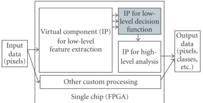
In this paper, we propose a method of automatic genera-tion of hardware implementagenera-tion of a particular decision rule. This paper focuses mainly on high-speed decisions (ap-proximately 15 to 20 nanoseconds per decision) which can be useful for high-resolution image segmentation (low-level decision function) or pattern recognition tasks in very large image databases. Our work—in grey in theFigure 1—is de-signed in order to be easily integrated in a system-on-chip, which can perform the full process: acquisition, feature

ex-traction, and classification, in addition to other custom data processing.

(2)

Input data (pixels)

Virtual component (IP) for low-level feature extraction

IP for low-level decision

function IP for high-level analysis Other custom processing

Single chip (FPGA)

Output data (pixels, classes, etc.)

Figure1: Principle of a decision function integrated in a system-on-chip.

register-transfer-level representation (RTL) [5], have been developed and which allow such a manual description to be avoided. Compilers are available for example for SystemC, Streams-C, Handel-C [6,7], or for translation of DSP bina-ries [8]. Our approach is slightly diﬀerent, since in the case of supervised learning, it is possible to compile the learning data in order to obtain the optimized architecture, without the need of a high-level language translation.

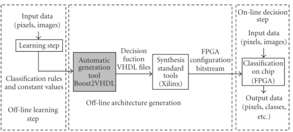
The aim of this work is to provide the EDA tool (Boost2VHDL, developed in C++) which generates auto-matically the hardware description of a given decision func-tion, while finding an eﬃcient tradeoﬀ between decision speed, classification performances, and silicon area which we will call hardware implementation cost denoted asλ. The de-velopment flow is depicted inFigure 2. The idea is to generate automatically the architecture from the learning data and the results of the learning algorithm.

The first process is the learning step of a supervised clas-sification method, which produces, oﬀ-line, a set of rules and constant values (built from a set of samples and their associated classes). The second step is also an oﬀ-line pro-cess. During this step, called Boost2VHDL, we built auto-matically from the previously processed rules the VHDL files implementing the decision function. In a third step, we use a standard implementation tool, producing the bit-stream file which can be downloaded in the hardware target. A new learning step will give us a new architecture. During the on-line process, the classification features and the decision func-tion are continuously computed from the input data, pro-ducing the output class (seeFigure 1).

This approach allows us to generate an optimized archi-tecture for a given learning result, but implies the use of a programmable hardware target in order to keep flexibility. Moreover, the time constraints for the whole process (around 20 nanoseconds per acquisition/feature extraction/decision) imply a high use of parallelism. All the classification features have to be computed simultaneously, and the intrinsic op-erations of the decision function itself have to be computed in parallel. This naturally led us using FPGA as a potential hardware target.

In recent years, FPGAs have become increasingly impor-tant and have found their way into system design. FPGAs are used during development, prototyping, and initial pro-duction and can be replaced by hardwired gate arrays

or application-specific component (ASIC) for high-volume production. This trend is enforced by rapid technological progress, which enables the commercial production of ever more complex devices [9]. The advantage of these compo-nents compared to ASIC is mainly their on-board reconfig-urability, and compared to a standard processor, their high level of potential parallelism [10]. Using reconfigurable ar-chitecture, it is possible to integrate the constant values in the design of the decision function (here for example the constants resulting from the learning step), optimizing the number of cells used. We consider here the slice (Figure 3) as the main elementary structure of the FPGA and the unit ofλ. One component can contain a few thousand of these blocks. While the size of these components is always increasing, it is still necessary to minimize the number of slices used by each function in the chip. This reduces the global cost of the sys-tem, increases the classification performance and the number of operators to be implemented, or allows the implementa-tion of other processes on the same chip.

We choose the well known Adaboost algorithm as the im-plemented classifier. The decision step of this classifier con-sists in a simple summation of signed numbers [11,12,13]. Introduced by Schapire in 1990, Boosting is a general method of producing a very accurate prediction rule by combining rough and moderately inaccurate “rules of thumb.” Most re-cent work has been on the “AdaBoost” boosting algorithm and its extensions. Adaboost is currently used for numerous researches and applications, such as the Viola-Jones face de-tector [14], or in order to solve the image retrieval problem [15] or the word-sense disambiguation problem [16], or for prediction in wireless telecommunications industry [17]. It can be used in order to improve classification performances of other classifiers such as SVM [18]. The reader will find a very large bibliography onhttp://www.boosting.org. Boost-ing, because of its interesting properties of maximizing mar-gins between classes, is one of the most currently used and studied supervised method in the machine learning commu-nity, with support vector machine and neural networks. It is a powerful machine learning method that can be applied directly, without any modification, to generate a classifier implementable in hardware, and a complexity/performance tradeoﬀis natural in the framework: Adaboost learning con-structs gradually a set of classifiers with increasing complex-ity and better performance (lower cross-validated error). All along this study, we kept in mind the necessity of obtaining high performances in terms of classification. We performed systematically measurements of classification errore(using a tenfold cross-validation protocol). Indeed, in order to follow real-time processing and cost constraints, we had to mini-mize the errorewhile minimizing the hardware implementa-tion costλand maximize the decision speed. The maximum speed has been obtained using a fully parallel implementa-tion.

(3)

Input data (pixels, images)

Learning step

Classification rules and constant values Oﬀ-line learning

step

Automatic generation

tool Boost2VHDL

Decision fuction VHDL files

Synthesis standard tools (Xilinx)

FPGA configuration

bitstream

Oﬀ-line architecture generation

On-line decision step Input data (pixels, images)

Classification on chip (FPGA) Output data (pixels, classes,

etc.)

Figure2: Development flow.

G4

G3

G2

G1

F4

F3

F2

F1

BX

LUT

Carry and control

LUT

Carry and control

D Q

EC

D Q

EC

YB Y YQ

XB X XQ

Figure3: Slice structure.

In the second part, we define a family of weak classifiers suitable to hardware implementation, based on the general concept of hyperrectangle. We present the algorithm which is able to find a hyperrectangle which minimizes the classi-fication error and allows us to find a good tradeoﬀbetween classification performance and the hardware implementation cost which we estimated. This method is based on a previous work: we have shown in [19,20] that it is possible to im-plement a hyperrectangle-based classifier in a parallel com-ponent in order to obtain the required speed. Then, we de-fine the global hardware implementation cost, taking into ac-count the structure of the Adaboost method and the struc-ture of the weak classifiers.

In the third part, results are presented: we applied the method on Gaussian distributions, which are often used in literature for performance evaluation of classifiers [21], and we presented results obtained on real databases coming from the UCI repository. Finally, we applied the method to an dustrial problem, which consists in the real-time visual in-spection of CRT cathodes. The aim is to perform a real-time image segmentation based on pixel classification. This seg-mentation is an important preprocessing used for detection of anomalies on the cathode.

The main contributions of this paper are the from-learning-data-to-architecture tool, and in the Adaboost pro-cess, the introduction of using hyperrectangles as a

possi-ble optimization of classification performances and hardware cost.

2. PROPOSED METHOD

2.1. Review of Adaboost

The basic idea introduced by Schapire and Freund [11,12, 13] is that a combination of single rules or “weak classifiers” gives a “strong classifier.” Each sample is defined by a feature vectorx=(x1,x2,. . .,xD)Tin aD-dimensional space and its

corresponding class:C(x)=y∈ {−1, +1}in the binary case. We define the weighted learning setSofpsamples as

S=x1,y1,w1

,x2,y2,w2

,. . .,xp,yp,wp

, (1)

wherewiis the weight of theith sample.

Each iteration of the process consists in finding the best possible weak classifier, that is, the classifier for which the error is minimum. If the weak classifier is a single threshold, all the thresholds are tested.

After each iteration, the weights of the misclassified ples are increased, and the weights of the well-classified sam-ple are decreased.

The final classyis given by

y(x)=sgn _T

t=1 αtht(x)

, (2)

where bothαtandht are to be learned by the boosting

pro-cedure presented inAlgorithm 1. The characteristics of the classifier we have to encode in the architecture are the coeﬃ -cientsαtfort=1,. . .,T, and the intrinsic constants of each

weak classifierht.

2.2. Parallel implementation of the global structure

The final decision function to be implemented (equation (2)) is a particular sum of products, where each product is made of a constant (αt) and the value−1 or +1 depending of the

output ofht. It is then possible to avoid computation of

(4)

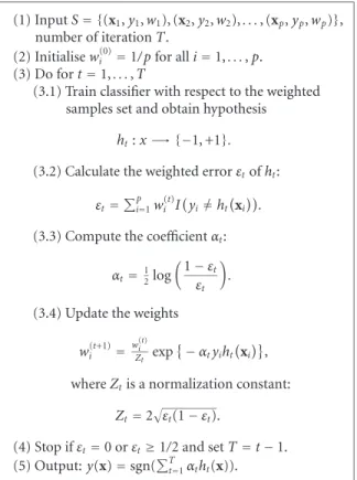
(1) InputS= {(x1,y1,w1), (x2,y2,w2),. . ., (xp,yp,wp)},

number of iterationT.

(2) Initialisewi(0)=1/ pfor alli=1,. . .,p.

(3) Do fort=1,. . .,T

(3.1) Train classifier with respect to the weighted samples set and obtain hypothesis

ht:x−→ {−1, +1}.

(3.2) Calculate the weighted errorεtofht:

εt=

p

i=1w

(t)

i I

yi=ht

xi

.

(3.3) Compute the coeﬃcientαt:

αt=12log

1−εt

εt

.

(3.4) Update the weights

wi(t+1)=w

(t) i

Zt exp

−αtyihtxi,

whereZtis a normalization constant:

Zt=2

εt(1−εt).

(4) Stop ifεt=0 orεt≥1/2 and setT=t−1.

(5) Output:y(x)=sgn(T_t=1αtht(x)).

Algorithm1: The boosting procedure.

In terms of slices, the hardware cost can be expressed as follows:

λ=(T−1)λadd+λT, (3)

whereλaddis the cost of an adder (which will be considered

as a constant here), andλT is the cost of the parallel

imple-mentation of the set of the weak classifiers:

λT = T

t=1

λt, (4)

whereλt is the cost of the weak classifierhtassociated to the

multiplexers. One can note that due to the binary nature of the output ofht, it is possible to encode the results of

addi-tions and subtracaddi-tions in the 16-bit LUT of FPGA, using the output of the weak classifiers as addresses (Figure 5). This is the first way to obtain an architecture optimized for a given learning result. The second way will be the implementation of the weak classifiers.

Since the classifierhtis usedTtimes, it is critical to

opti-mize its implementation in order to miniopti-mize the hardware cost. As a simple classifier, single parallel-axis threshold is of-ten used in the literature about Boosting. However, this type of classifier requires a large number of iterationsTand hence the hardware cost increases (as it depends on the number of additions to be performed in parallel). To increase the com-plexity of the weak classifier allows faster convergence, and then minimizes the number of additions, but this will also increase the second member of the equation. We have then to find a tradeoﬀbetween the complexity ofhtand the

hard-ware cost.

x h0

+α0 −α0

MUX . . .

ht

+αt −αt

MUX

Set of adders sgn

y

Figure4: Parallel implementation of Adaboost.

16 bit LUT

h0

h1

h2

h3

+α0+α1+α2+α3

+α0+α1+α2−α3

+_.α0+α1−α2−α3

. .

−α0−α1−α2−α3

. . . h0 h1 h2 h3

16 bit LUT +α0+α1+α2+α3

+α0+α1+α2−α3

+_.α0+α1−α2−α3

. .

−α0−α1−α2−α3

h4

h5

h6

h7

16 bit LUT +α4+α5+α6+α7

+α4+α5+α6−α7

+_.α4+α5−α6−α7

. .

−α4−α5_.−α6−α7

. . Bit 0 Bit 7 Bit 0 Set of adders

Figure5: Details of the first stage: coding constants in the architec-ture of the FPGA.

3. WEAK CLASSIFIER DEFINITION AND

IMPLEMENTATION OF THE WHOLE DECISION FUNCTION

3.1. Choice of the weak classifier: definitions

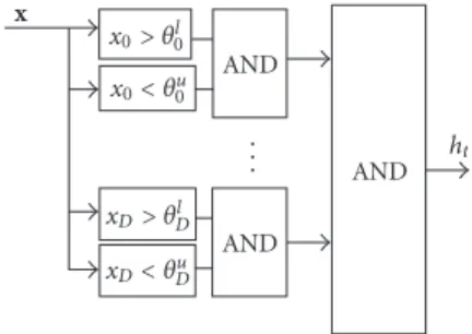
It has been proved in the literature that decision trees based on hyperrectangles (or union of boxes) instead of a sin-gle threshold give better results [22]. Moreover, the decision function associated with a hyperrectangle can be easily im-plemented in parallel (Figure 6).

However, there is no algorithm on the complexity ofD

which allows us to find the best hyperrectangle, that is, min-imising the learning error. Therefore, we will use a subopti-mum algorithm to find it.

We defined the generalized hyperrectangle as a setH of 2Dthresholds and a classyH, withyH∈ {−1, +1}:

H=θl

1,θu1,θl2,θ2u,. . .,θDl,θuD,yH

, (5)

whereθkl andθuk are, respectively, the lower and upper

(5)

x

x0> θ0l

x0< θu0

xD> θDl

xD< θDu

AND . . . AND

AND ht

Figure6: Parallel implementation ofht.

function is

hH(x)=yH⇐⇒ D

d=1

xd> θdl

andxd< θdu

,

hH(x)= −yH otherwise.

(6)

This expression, where product is the logical operator, can be simplified if some of these limits are rejected to the in-finite (or 0 and 255 in case of a byte-based implementation). Comparisons are not necessary in this case since the result will be always true. It is particularly important for minimiz-ing the final number of used slices. Two particular cases of hyperrectangles have to be considered.

(i) The single threshold:

Γ=θd,yΓ

, (7)

whereθdis a single threshold,d∈ {1,. . .,D}, and the

deci-sion function is

hΓ(x)=yΓ⇐⇒xd< θd,

hΓ(x)= −yΓ otherwise.

(8)

(ii) The single interval:

∆=θl d,θud,y∆

, (9)

where the decision function is

h∆(x)=y∆⇐⇒xd> θdl

andxd< θdu

,

h∆(x)= −y∆ otherwise. (10)

In these two particular cases, it is easy to find the optimum hyperrectangle, because each feature is considered indepen-dently from the others. The optimum is obtained by comput-ing the weighted error for each possible hyperrectangle and choosing the one for which the error is minimum.

In the general case, one has to follow a particular heuris-tic given a suboptimum hyperrectangle. A family of such classifiers have been defined, based on the NGE algorithm

described by Salzberg [23] whose performance was

com-pared to the KNN method of Wettschereck and Dietterich [24]. This method divides the attribute space into a set of hyperrectangles based on samples. The performance of our

x2

x1

x5

x4

x6

x0

x8

θu 41

x2

x7

x3

x1

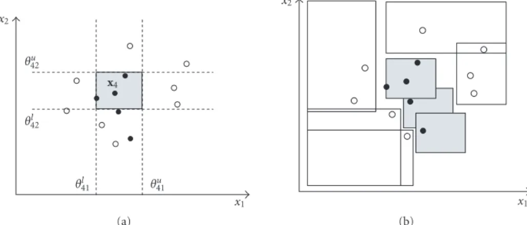
Figure 7: Determination of the first limit ofH(x4). In this case, i=4,z=7, ˜k=1,θu

41=R(x71−x41).

own implementation was studied in [25]. We will review the principle of the hyperrectangle determination in the next section.

3.2. Review of the hyperrectangle-based method

The core of the strategy is the hyperrectangles setSH

deter-mination from a set of samplesS.

The basic idea is to build around each sample{xi,yi} ∈S

a box or hyperrectangleH(xi) containing no sample of

op-posite classes (see Figures7and8):

Hxi)=

θil1,θui1,θil2,θui2,. . .,θiDl ,θuiD,yi

. (11)

The initial value is set to 0 for all lower bounds and 255 for all upper bounds.

In order to measure the distance between two samples in the feature space, we use the “max” distance defined by

d∞xi,xj

= max

k=1,...,D

_x_ik₋_x_jk_. ₍₁₂₎

The use of this distance instead of the Euclidean dis-tance allows building easily hyperrectangle instead of hyper-sphere. For all axes of the feature space, we determine the sample{xz,yz},yz = yi, as the nearest neighbour ofxi

be-longing to a diﬀerent class:

z=arg min

j

d∞xi,xj

. (13)

The threshold defining one bound of the box is perpendicu-lar to the axis ˜kfor which the distance is maximum:

˜

k=arg max

k

_x_ik₋_x_zk_. (14)

Ifxik˜> xzk˜, we compute the lower limitθli_k˜=R(xik˜−xzk˜). In

the other case, we compute the upper limitθu_i_k˜=R(xz_k˜−x_i˜_k).

The parameterRshould be less than or equal to 0.5. This constraint ensures that the hyperrectangle cannot contain any sample of opposite classes.

The procedure is repeated until finding all the bounds of

(6)

x2

θu 42

θl 42

x4

θl41 θ41u

x1

(a)

x2

x1

(b)

Figure8: Hyperrectangle computation. (a) Determination ofH(x4). (b) Hyperrectangles obtained after merging step.

(3.1.1) Initializeεmin=1.0

(3.1.2) Do for each classy= −1, 1 Do fori=0,. . .,q₍_y₎

Do forj=i+ 1,. . .,q₍_y₎ BuildHtemp=Hi∪Hj

ComputeεHthe weighed

error based onHtemp

ifεH< εminthenHopt= HtempandεH=εmin

endj

endi

endy

(3.1.3) Output:hH=Hopt

Algorithm2

During the second step, hyperrectangles of a given class are merged together in order to eliminate redundancy (hy-perrectangles which are inside of other hy(hy-perrectangles of the same class). We obtain a setSHof hyperrectangles:

SH=

H1,H2,. . .,Hq

. (15)

We evaluated the performance of this algorithm in various cases, using theoretical distributions as well as real sampling [19]. We compared the performance with neural networks, the KNN method, and a Parzen’s kernel-based method [26]. It clearly appears that the algorithm performs poorly when the interclass distances are too small: an important number of hyperrectangles are created in the overlap area, slowing down the decision or increasing the implementation cost. However, it is possible to use the hyperrectangle generated as a step of the Adaboost process, selecting the best one in terms of classification error.

3.3. Boosting general hyperrectangle and combination of weak classifiers

FromSHwe have to build one hyperrectangleHopt

minimiz-ing the weighted error. To obtain this result, we merge hy-perrectangles following a one-to-one strategy, thus building

q =q(q−1) new hyperrectangles. We keep the hyperrect-angle which gives the smallest weighted error.

For each iteration of the (3.1) Adaboost step, we design Algorithm 2.

(3) Do fort=1,. . .,T

(3.1) Train classifier with respect to the weighted samples set{S,d(t)_}_{and obtain the three}

hypothesishΓ,h∆, andhH

(3.2) Calculate weighted errorsεΓ,ε∆, andεH

introduced by each classifier

(3.3) Choosehtfrom{hΓ,h∆,hH}for whichεt=

min(εΓ,ε∆,εH)

(3.4) Estimateλ

Algorithm3

In order to optimize the final result, it is possible to com-bine the previous approaches, finding for each iteration the best weak classifier between the single threshold hΓ, the

in-tervalh∆, and the general hyperrectanglehH. Step (3) of the

Adaboost algorithm is illustrated inAlgorithm 3. As we will see in the results presented inSection 4, this strategy allows minimizing the number of iterations, and thus minimizing the final hardware cost in most of the case, even if the hard-ware cost of the implementation of an hyperrectangle is lo-cally more important than the cost of the implementation of a single threshold.

3.4. Estimation of the hyperrectangle hardware implementation cost

As the elementary structure of the hyperrectangle is based on numerous comparisons performed in parallel (Figure 6), it is necessary to optimize the implementation of the comparator. It is possible to estimate the hardware implementation cost ofhttaking into account that we can code the constant

values of the decision function into the final architecture, us-ing the advantage of FPGA-based reconfigurable computus-ing. Indeed, the binary resultLBof the comparison of the variable

byteAand the constant byteBis a functionFBof the bits of A:

LB=FB

A7,A6,. . .,A0

. (16)

We consider for exampleB=151, 10010111 in binary, then, where “∗” is the logic operator AND, “+” is the logic opera-tor OR:

L151=A7∗

A6+

A5+

A4∗A3

, (17)

(7)

More generally, we can writeLBas follows (for any byte Bsuch that 0< B <255):

LB=A7@

A6@

A5@

A4@

A3@

A2@

A1@

A0@0

.

(18)

The @ operator denotes either the AND operator or the OR operator, depending on the position of @ and the value of

B. In the worst case, the particular structure ofLB can be

stored in two cascaded lookup tables (LUT) of 16 bits each (one slice).

We have coded in the tool Boost2VHDL a function which automatically generates a set of VHDL files: this is the hard-ware description of the decision functions ht given the

re-sult of a training step (i.e., given the hyperrectangles limits). The files generated are used in the parallel architecture de-picted in theFigure 5, which is also automatically generated using the constants of the Boosting process. We then have used a standard synthesizer tool for the final implementation in FPGA.

In the case of single threshold,λt=1, for allt∈[1,T]. In

the case of interval,λt≤2. In the case of general

hyperrectan-gle, the decision rule requires in the worst case 2 comparators per hyperrectangle and per feature:λt≤2D.

3.5. Estimation of the global Adaboost implementation

Considering that some limits of the general hyperrectangle can be rejected to the “infinite,” the general cost of the whole Adaboost-based decision can be expressed as follows:

λ≤(T−1)λadd+µT, withµ≤2D, (19)

whereµis the sum of the number of lower limits of hyper-rectangles which are greater than 0, and the number of upper limits which are lower than 255.

The implementation is eﬃcient in terms of real-time computational for a reasonable value ofD. In order to obtain very fast classification (around 10 nanoseconds per decision), we considered here only the full parallel implementation of all the process, including the classification features extraction (Dfeatures have to be computed in parallel). We limited our investigation here toD=64.

One can note also that the hardware cost here is di-rectly linked to the discrimination power of the classification features. In the classification framework, it is a well-known problem that is it critical to find eﬃcient classification fea-tures in order to minimize classification error. Here, the bet-ter the classification features are selected, the fasbet-ter the Boost-ing converges (Twill be low), and the lower will be the hard-ware cost.

Moreover, an originality of this work is to allow the user to choose himself to control the Boosting process modifying the stopping criterion in step (4), and introducing a maxi-mum hardware costλmax. The step becomes

(4) Stop ifεt=0 orεt≥1/2 orλ≥λmaxand setT=t−1.

Finally, the user can choose the best tradeoﬀbetween classification error and hardware implementation cost for its application. Moreover, compared to a standard VHDL de-scription of a classifier, our generated architecture is opti-mized for the user’s application, since a specific VHDL de-scription is generated for each process of training.

4. RESULTS

We applied our method in diﬀerent cases. This first one is based on Gaussian distributions and in a two-dimensional space. We used this example in order to illustrate the method and the improvement given by hyperrectangle in terms of performance of classification.

The second series of examples, based on real databases coming from the UCI repository, is more significant in terms of hardware implementation, since they are performed in higher-dimensional spaces (until D = 64, this can be seen as a reasonable limit for a full parallel implementation).

The last example is from an industrial problem of qual-ity control by artificial vision, where anomalies are to be de-tected in real time on metallic parts. The problem we focus on here is the segmentation step, which can be performed using pixelwise classification.

For each example, we also provide the result of a deci-sion based on SVM developed by Vladimir Vapnik in 1979, which is known as one of the best classifiers, and which can be compared with Adaboost on the theoretical point of view. At the same time, SVM can achieve good performance when applied to real problems [27,28,29,30]. In order to compare the implementation cost of the two methods, we evaluated the hardware implementation cost of SVM as

λSVM72(3D−1)Ns+ 8, (20)

where Ns is the total number of “support vectors” deter-mined during the training step. We used here an RBF-based kernel, using distanceL1. While the decision function seems to be similar to the Adaboost one, the cost is here mainly higher because of multiplications; even if the exponential function can be stored in a particular lookup table to avoid computation, the kernel productKrequires some multipli-cations and additions; the final decision function requires at least one multiplication and one addition per support vector:

C(x)=sgn _Ns

i=1 yiαi·K

si,x

+b

. (21)

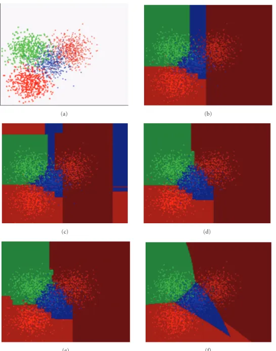
4.1. Experimental validation using Gaussian distributions

(8)

(a) (b)

(c) (d)

(e)

.3

(f)

Figure9: Example inD=2, with 4 classes. (a) Original 4-class distribution, and boundaries with (b) single threshold, (c) single interval, (d) general hyperrectangle, (e) combination, and (f) SVM (RBF).

Results in terms of classification error are given in Table 1. As expected, the method works well in all the cases but the XOR one using single threshold or interval. We re-ported also the estimated number of slices, but in this par-ticular case of a two-dimensional problem, it is clear that it is also possible to store the whole result of the SVM classifier in a single RAM, for example. However, this test well illus-trates how it is possible to approximate complex classifica-tion boundaries with a single set of hyperrectangles.

4.2. Experimental validation using real databases

In order to validate our approach, we evaluate the hard-ware implementation cost of classification of databases from

the UCI database repository. Results are summarized in the Table 2. We give the classification errore(%), the estimated number of slices (λ), a comparison with the decision time computation Pc, obtained with a standard PC (2.5 GHz) in the case of combination of best weak classifiers, and the speedup Su = Pc/0.01 of hardware computation, obtained with a 50 MHz clock.

(9)

Table1: Error using Gaussian distributions.

Distribution D Classes Optimum SVM (RBF) Threshold Interval Hyperrectangle Combination

e(%) e(%) λSVM e(%) λ e(%) λ e(%) λ e(%) λ

4 Gaussians 2 4 13 13.02 59048 14.8 181 13.62 386 13.22 46 13.2 32

Xor 2 2 4.4 4.6 129248 47.65 41 49 49 5.25 11 5.25 8

Table2: Results on real databases.

Distribution D C SVM (RBF) Threshold Interval Hyperrectangle Combination

e(%) λSVM e(%) λ e(%) λ e(%) λ e(%) λ Pc (µs) Su

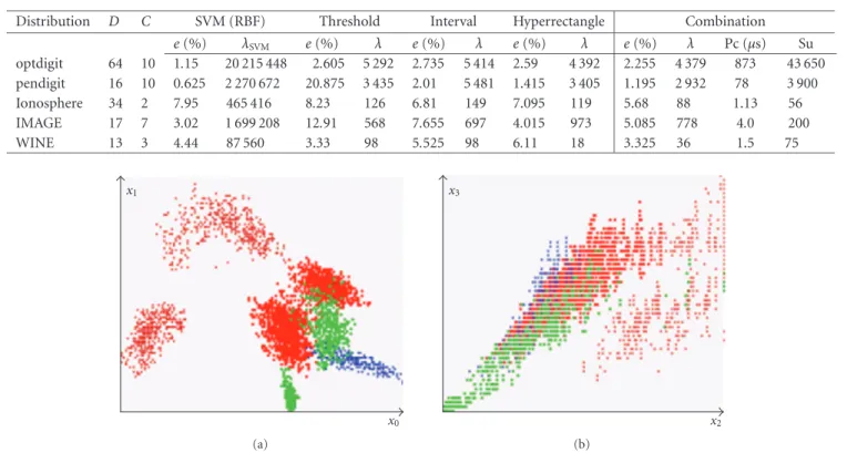
optdigit 64 10 1.15 20 215 448 2.605 5 292 2.735 5 414 2.59 4 392 2.255 4 379 873 43 650 pendigit 16 10 0.625 2 270 672 20.875 3 435 2.01 5 481 1.415 3 405 1.195 2 932 78 3 900 Ionosphere 34 2 7.95 465 416 8.23 126 6.81 149 7.095 119 5.68 88 1.13 56 IMAGE 17 7 3.02 1 699 208 12.91 568 7.655 697 4.015 973 5.085 778 4.0 200

WINE 13 3 4.44 87 560 3.33 98 5.525 98 6.11 18 3.325 36 1.5 75

x1

x0

(a)

x3

x2

(b)

Figure10: Extracted features for segmentation. (a)x0andx1projections. (b)x2andx3projections.

Considering the diﬀerent results of our Adaboost implemen-tation, it appears clearly that the combination of the three types of weak classifiers gives the better results. The opt-digit and the penopt-digit cases can be solved using half of a cir-cuit XCV600 of the VirtexE family, for example, while all the other cases can be implemented in a single low-cost chip.

Moreover, the classification error of the Adaboost-based classifier is very close to the SVM one.

Due to the parallel structure of our hardware implemen-tation, the speedup is really important when the numbers of featuresDand classesCare high. Even if we reduce for ex-ample the frequency to 1 MHz in the case “optdigit” in order to follow a slower feature extraction, the speedup is still more than 800 compared to a standard software implementation.

Our system can also be used as a coprocessor embedded in a PCI-based board, limited to 33 MHz (32 bit data, allow-ing the parallel transmission of only 4 features from another board dedicated to data acquisition and features computa-tion). The speedup in the case of image segmentation could be here for example:

Su=Pc/0.03

D/4 = 4/0.03

17/4 31. (22)

However, the main interest of our method is to be integrated in a single component together with the other processes, as depicted inFigure 1.

4.3. Example of industrial application: image segmentation

We applied the previous method in order to perform an im-age segmentation step of a quality control process. The aim here is to detect some anomalies on manufactured parts, fol-lowing the rate of 10 pieces per second. The resolution of the processed area is 300×300 pixels. The whole control (ac-quisition, feature extraction, segmentation, analysis, and fi-nal classification of the part) has to be achieved in less than 100 milliseconds. Thus, feature extraction and pixelwise clas-sification have to be achieved in less than 1 microsecond.

(10)

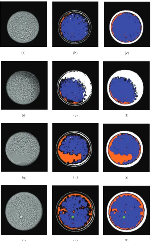
(a) (b) (c)

(d) (e) (f)

(g) (h) (i)

(j) (k) (l)

Figure11: Example of segmentation results using threshold and hyperrectangles. (Left column) Original image with (a) denoting defect-free cathode, (d) missing material, (g) smooth area, and (j) bump. (Middle column) Image segmented using a single threshold. (Right column) Image segmented using hyperrectangles.

We depicted some examples of segmentation results in Figure 11. It is clear that the anomalies are better segmented using hyperrectangles than other weak classifiers. These re-sults are confirmed by the cross-validated error presented in theTable 3. In this case, the better tradeoﬀbetween classi-fication performance and hardware implementation cost is obtained using the combination of diﬀerent weak classifiers.

The estimated number of needed slices is less than 700 for a classification errore=2.44%, which is very close to the error obtained using SVM, and this for a very lower hardware cost than the SVM one.

(11)

Table3: Results on industrial application.

Distribution D Classes SVM (RBF) Threshold Interval Hyperrectangle Combination

e(%) λ e(%) λ e(%) λ e(%) λ e(%) λ Pc (µs) Su

Cathode 4 4 1.44 234440 8.16 434 6.15 467 2.41 726.5 2.44 677 2.7 135

account). The speedup of the hardware implementation— more than 100 for a 50 MHz clock—allows to follow these real-time constraints.

5. CONCLUSION

We have developed a method and EDA tool, called Boost2VHDL, allowing automatic generation of hardware implantation of a particular decision rule based on the Ad-aboost algorithm, which can be applied in many pattern recognition tasks, such as pixelwise image segmentation, character recognition, and so forth. Compared to a standard VHDL-based description of a classifier, the main novelty of our approach is that the tool allows the user to find auto-matically an appropriate tradeoﬀbetween classification per-formances and hardware implementation cost. Moreover, the generated architecture is optimized for the user’s application, since a specific VHDL description is generated for each pro-cess of training.

We experimentally validated the method on theoretical distributions as well as real cases, coming from standard datasets and from an industrial application. The final error of this implemented classifier is close to the error obtained using an SVM-based classifier, which is often used in the lit-erature as a good reference. Moreover, the method is really easy to use, since the only parameter to find is the choice of the weak classifier, the Rvalue of the hyperrectangle-based method, or the maximum hardware cost allowed for the ap-plication. We are currently finalizing the development tool which will allow the development of the whole implementa-tion process, from the learning set definiimplementa-tion to FPGA-based implementation using automatic VHDL generation, and we will use it in the near future in order to speed up some pro-cesses using a coprocessing PCMCIA board based on a Vir-tex2 from Xilinx. Our future work will be the integration of this method as a standard IP generation tool for classifica-tion.

ACKNOWLEDGMENT

The author was supported by The Czech Academy of Sci-ences under project 1ET101210407.

REFERENCES

[1] P. Lysaght, J. Stockwood, J. Law, and D. Girma, “Artificial neu-ral network implementation on a fine-grained FPGA,” inProc. 4th International Workshop on Field-Programmable Logic and Applications (FPL ’94), R. Hartenstein and M. Z. Servit, Eds., pp. 421–431, Prague, Czech Republic, September 1994.

[2] Y. Taright and M. Hubin, “FPGA implementation of a multi-layer perceptron neural network using VHDL,” inProc. 4th In-ternational Conference on Signal Processing (ICSP ’98), vol. 2, pp. 1311–1314, Beijing, China, December 1998.

[3] C. M. Bishop,Neural Networks for Pattern Recognition, Oxford University Press, Oxford, UK, 1995.

[4] R. A. Reyna-Rojas, D. Dragomirescu, D. Houzet, and D. Es-teve, “Implementation of the SVM generalization function on FPGA,” inProc. International Signal Processing Conference (ISPC ’03), pp. 147–153, Dallas, Tex, USA, March 2003. [5] G. DeMichelli, Synthesis and Optimization of Digital Circuits,

McGraw Hill, New York, NY, USA, 1994.

[6] J. Frigo, M. Gokhale, and D. Lavenier, “Evaluation of the stream-C C-to-FPGA compiler: an application perspective,” inProc. 9th ACM/SIGDA International Symposium on Field-Programmable Gate Arrays (FPGAs ’01), pp. 134–140, Mon-terey, Calif, USA, February 2001.

[7] I. Page, “Constructing hardware-software systems from a sin-gle description,”Journal of VLSI Signal Processing, vol. 12, no. 1, pp. 87–107, 1996.

[8] G. Mittal, D. C. Zaretsky, X. Tang, and P. Banerjee, “Automatic translation of software binaries onto FPGAs,” inProc. 41st Design Automation Conference (DAC ’04), pp. 389–394, San Diego, Calif, USA, June 2004.

[9] R. Enzler, T. Jeger, D. Cottet, and G. Tr¨oster, “High-level area and performance estimation of hardware building blocks on FPGAs,” inProc. 10th International Workshop on Field-Programmable Logic and Applications (FPL ’00), vol. 1896 of Lecture Notes in Computer Science, pp. 525–534, Springer, Vil-lach, Austria, August 2000.

[10] S. Hauck, “The roles of FPGAs in reprogrammable systems,” Proc. IEEE, vol. 86, no. 4, pp. 615–638, 1998.

[11] R. E. Schapire, “The strength of weak learnability,” Machine Learning, vol. 5, no. 2, pp. 197–227, 1990.

[12] Y. Freund and R. E. Schapire, “A decision-theoretic general-ization of on-line learning and an application to boosting,” Journal of Computer and System Sciences, vol. 55, no. 1, pp. 119–139, 1997.

[13] R. E. Schapire, “The boosting approach to machine learn-ing: an overview,” inProc. MSRI Workshop on Nonlinear Esti-mation and Classification, pp. 149–172, Berkeley, Calif, USA, 2002.

[14] P. Viola and M. Jones, “Rapid object detection using a boosted cascade of simple features,” inProc. IEEE Computer Soci-ety Conference on Computer Vision and Pattern Recognition (CVPR ’01), vol. 1, pp. 511–518, Kauai, Hawaii, USA, Decem-ber 2001.

[15] K. Tieu and P. Viola, “Boosting image retrieval,”International Journal of Computer Vision, vol. 56, no. 1–2, pp. 17–36, 2004. [16] G. Escudero, L. M`arquez, and G. Rigau, “Boosting applied to

word sense disambiguation, LNAI 1810,” inProc. 12th Euro-pean Conference on Machine Learning (ECML ’00), pp. 129– 141, Barcelona, Spain, 2000.

(12)

[18] G. Rätsch, S. Mika, B. Schölkopf, and K.-R. Müller, “Con-structing boosting algorithms from SVMs: an application to one-class classification,” IEEE Trans. Pattern Anal. Machine Intell., vol. 24, no. 9, pp. 1184–1199, 2002.

[19] J. Mitéran, P. Gorria, and M. Robert, “Classification géomét-rique par polytopes de contraintes intégration et perfor-mances,” Traitement du Signal, vol. 11, no. 5, pp. 393–408, 1995.

[20] M. Robert, P. Gorria, J. Mit´eran, and S. Turgis, “Architectures for a real time classification processor,” inProc. IEEE Custom Integrated Circuits Conference (CICC ’94), pp. 197–200, San Diego, Calif, USA, May 1994.

[21] R. O. Duda and P. E. Hart, Pattern Classification and Scene Analysis, Wiley, New York, NY, USA, 1973.

[22] I. De Macq and L. Simar, “Hyper-rectangular space partition-ning trees, a few insight,” discussion paper 1024, Universit´e Catholique de Louvain, Belgium, 2002.

[23] S. Salzberg, “A nearest hyperrectangle learning method,” Ma-chine Learning, vol. 6, no. 3, pp. 251–276, 1991.

[24] D. Wettschereck and T. Dietterich, “An experimental compar-ison of the nearest-neighbor and nearest-hyperrectangle algo-rithms,”Machine Learning, vol. 19, no. 1, pp. 5–27, 1995. [25] J. Mit´eran, J. P. Zimmer, F. Yang, and M. Paindavoine,

“Ac-cess control: adaptation and real-time implantation of a face recognition method,” Optical Engineering, vol. 40, no. 4, pp. 586–593, 2001.

[26] P. Geveaux, S. Kohler, J. Miteran, and F. Truchetet, “Analy-sis of compatibility between lighting devices and descriptive features using Parzen’s Kernel: application to flaw inspection by artificial vision,” Optical Engineering, vol. 39, no. 12, pp. 3165–3175, 2000.

[27] V. Vapnik,The Nature of Statistical Learning Theory, Springer-Verlag, New York, NY, USA, 1995.

[28] B. Sch¨olkopf, A. Smola, K.-R. M¨uller, C. J. C. Burges, and V. Vapnik, “Support vector methods in learning and feature extraction,” Australian Journal of Intelligent Information Pro-cessing Systems, vol. 1, pp. 3–9, 1998.

[29] K. Jonsson, J. Kittler, Y. P. Li, and J. Matas, “Support vector machines for face authentication,” inProc. British Machine Vision Conference (BMVC ’99), T. Pridmore and D. Elliman, Eds., pp. 543–552, London, UK, September 1999.

[30] M. A. Hearst, B. Sch¨olkopf, S. Dumais, E. Osuna, and J. Platt, “Trends and controversies - support vector machines,” IEEE Intell. Syst., vol. 13, no. 4, pp. 18–28, 1998.

J. Mit´eranis an Associate Professor (HDR) at Laboratory Le2i, the University of Bur-gundy. He is involved in research about real-time implementation of pattern recognition algorithms, using reconfigurable comput-ing. He is responsible for relationship be-tween Le2i and industrial partners, and he is on the program committee of international conferences such as HSPP, QCAV, SPIE Ma-chine Vision Applications in Industrial

In-spection, and ECCV Workshop Applications of Computer Vision 2004.

J. Matasgraduated (with honours) in tech-nical cybernetics from the Czech Techni-cal University in Prague, Czech Repub-lic, in 1987, and received his Ph.D. degree from the University of Surrey, UK, in 1995. He has published more than 100 papers in refereed journals and conferences. He was awarded the science paper prize at the British Machine Vision Conference in 2002 and “The best scientific results of the Czech

Technical University Prize” in 2003. He is on the program commit-tee of a number of international conferences (ICPR, NIPS, CVPR, Face and Gesture Recognition, Audio- and Video-based Biomet-ric Person Authentication). Dr. Matas was a Program Cochair for ECCV 2004—European Conference on Computer Vision.

E. Bourennanereceived the Ph.D. degree in automatics and image processing from the Le2i laboratory, the University of Bur-gundy in 1994. He is currently a Professor at the University of Burgundy. His research interests are mainly in real-time image pro-cessing. He is the President of the Program Committee of the AAA 2005 Workshop.

M. Paindavoineis a Professor at the Uni-versity of Burgundy. He is teaching signal and image processing in the Engineering School ESIREM and IUP “Electronique et Image.” He is the Head of the Laboratory Le2i (UMR CNRS 5158). His research in-terests are mainly in hardware implemen-tation of signal and image processing us-ing “ad´equation algorithmes architectures” methodology. He is on the program

com-mittee of a number of international conferences (GRETSI, HSPP, QCAV, etc.)

J. Dubois received a Ph.D. degree from the University Jean Monnet of Saint Eti-enne. During his Ph.D., he developed a new image processing architecture named “Round-About” for real-time motion mea-surements. This architecture has been ap-plied to measurement in fluid mechanics more precisely particle image velocimetry (PIV) in the University of Saint Etienne, France, in collaboration with the Image