111Equation Chapter 1 Section 1Expected Utility Theory with Imprecise Probability Perception
Explaining Preference Reversals
Oben K Bayrak
Centre for Environmental and Resource Economics, Umeå, Sweden
PhD, (corresponding author), Department of Forest Economics, SLU and CERE (Center for Resource and Environmental Economics), Skogsmarksgränd, Umeå, 901 83, Sweden, [email protected].
John D Hey
Department of Economics, University of York, York, UK
Expected Utility Theory with Imprecise Probability Perception
Explaining Preference Reversals
This paper presents a new model for decision-making under risk, which provides an explanation for empirically-observed Preference Reversals. Central to the theory is the incorporation of probability perception imprecision, which arises because of individuals’ vague understanding of numerical probabilities. We combine this concept with the use of the Alpha EU model and construct a simple model which helps us to understand anomalies, such as preference reversals and valuation gaps, discovered in the experimental economics literature, that standard models cannot explain.
Keywords: Alpha EU model, Anomalies in Expected Utility Theory; Decision under Risk; Imprecise Probability Perceptions; Preference Reversals Valuation Gaps.
JEL Classification: D81
Word count
1. Introduction
are almost identical under the different representations (See Budescu and Wallsten (1990), Wallsten et al (1986) and Bisantz et al (2005) for further evidence). Wallsten and Budescu (1995) explain that the similarity of behaviour under different representation modes is due to similarities in the vague understanding of probabilities. We therefore argue that a numerical, objective, probability corresponds to a range of probabilities and subjects use this range in their calculations. There is also implicit evidence from Plott and Zeiler (2005) and Isoni et al (2011) who find that the endowment effect is observed only for lottery tickets, but not for ordinary market goods such as mugs and candies.
Zimmer (1984) introduced a useful insight from an evolutionary perspective: he noted that the probability concept in a numerical sense is a relatively new concept, appearing as recently as the 17th century. However, people were communicating uncertainty via verbal expressions long
before probability was codified in mathematical terms. Zimmer further suggested that people process uncertainty in a verbal manner and make their decisions based on this processed information, not on the numerical information. We therefore assume that decision makers map any given objective probability into an interval. This implies that people end up with a range of probabilities and use this range in their decision-making.
This is the central point. To make the implications operationisable, we need to add in some theory as to how the decision-maker (DM) processes the interval probabilities. To do this, we use the Alpha EU Model (Arrow and Hurwicz 1972).
2. The Model
(x,0;p) which pays off x if s occurs and nothing otherwise, where s has probability p of occurring. We assume that u(x) ≥ u(0) where u(.) is the individual’s Neumann-Morgenstern utility function.
The crucial point of our theory is that the individual evaluates a risky prospect imprecisely due to his or her vague perception of probabilities; p is mapped to a range [p-βp,p+βp], where βp is
the imprecision level; our theory postulates that this βp is a function of p (the objective
probability) and a parameter which captures the individual-specific sophistication level ψ. A relatively unsophisticated individual would display a relatively high imprecision βp. In contrast,
stock brokers and gamblers, who are more familiar with the concept of probability, should exhibit a lower value of βp.
As far as the shape of βp as a function of p and ψ is concerned we assume that individuals
exhibit no imprecision if the probability is 0 or 1 since the events occurring with these probabilities are not probabilistic events. Secondly, imprecision reaches a maximum at 0.5 because it implies the event is neither likely nor unlikely. Finally, for simplicity, we assume that β(p,ψ) is symmetric around p=0.5. A simple example of such a function is β = ψp(1-p) which we use later.
As far as the individual is concerned, the lower bound of the expected utility of a two-outcome lottery is calculated by allocating probability p-β to state s (and probability 1-p+β to its complement), and the upper bound is calculated by assigning probability p+β to state s(and probability 1-p-β to its complement). To simplify the exposition we use the CRRA function u(x)=xr(so u(0)=0). Hence the lower and upper bounds of the expected utilities from a lottery X
= (x,0;p) are
EUU(X) = (p+βp)u(x) = (p+βp)xr
Now we need to add in our preference functional. As noted earlier we use the Alpha EU model. This is appropriate under ‘complete ignorance’, where the DM does not have any information as to which probability in the range is the true one. The Alpha EU is given by a weighted average of the worst and best expected utilities1:
AEU(X) = α EUL(X) + (1-α) EUU(X)
In a choice task between lotteries A = (x,0;p) and B = (y,0;q), the DM chooses A if αEUL(A) +(1-α)EUU(A) > αEUL(B) +(1-α)EUU(B) and B otherwise, and is indifferent if these expressions are the
same. The critical value of α, α*, for determining indifference is given by α*(p-βp)xr +(1- α*)(p+βp)xr = α*(q-βq)yr +(1- α*)(q+βq)yr
that is by
(1)
If α is above this, A is chosen; if below B is chosen.
When we come to valuations we need to tell a different story. Let us consider Willingness-to-Accept (WTA)2. Imagine that the individual owns the A lottery and is asked the minimum
amount for which he or she would sell it – the WTAA. If it is sold the individual has WTAA, and
the worst thing that can ‘happen’ to the individual is that the lottery would have paid out x, and the best thing that can ‘happen’ to the individual is that the lottery would have paid out 0. So the pessimist attaches weight p+β to the possibility of getting x, while the optimist attaches weight p-β. So EUL(A) = (p+βp)xr and EUU(A) = (p-βp)xr.
Using u(WTAA) = α EUL(A) + (1-α) EUU(B) we get
1 To clarify any possible confusion, we would like to note that in Hurwicz model, α represents the optimism of the decision maker, whereas in the decision making under ambiguity literature, in particular Alpha EU, it represents the pessimism. Here we follow the ambiguity literature’s convention rather than Hurwicz’s convention, and ascribe a negative meaning to the α parameter.
Similarly for B:
The critical value for (that where WTAA=WTAB) is:
(2) If α is above this α**, WTAA<WTAB; if below, WTAA>WTAB.
3. Explaining Preference Reversals
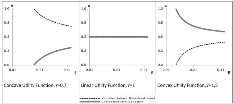
We now explore the implications of our theory. We present three cases which depend on the curvature of the utility function. Consider Figure 1, where A=(1.25,0;0.8)B=(5.0;0.2)3.
Figure 1: Where Preference Reversals might appear
0.01 0.21 0.41
0.0 0.3 0.5 0.8 1.0 β α
0.01 0.21 0.41
0.0 0.3 0.5 0.8 1.0 β α
0.01 0.21 0.41
0.0 0.3 0.5 0.8 1.0 β α
Concave Utility Function, r=0.7 Linear Utility Function, r=1 Convex Utility Function, r=1,3
0.01 0.21 0.41
0.0 0.5 1.0
Valuation (above: B is valued more) Choice (above: A is chosen)
A standard preference reversal occurs when the A-bet is chosen over the B-bet but the WTA for the A-bet is less than that for the B-bet. The solid line is the α*boundary and the dashed line the α**boundary. Above the solid line A is chosen and above the dashed line B is valued
higher; the region between the two lines is the consistency range where the chosen bet is valued more highly. For a linear utility function, in the case of imprecision (β>0), a standard Preference Reversal occurs if α>0.5; when it is lower than 0.5, the model predicts a non-standard Preference Reversal. The intuition behind this is that, unlike Expected Utility Theory, risk attitudes are not solely determined by the curvature of the utility function. In other words, in Expected Utility Theory, a linear utility function implies risk neutrality, but in our model it does not necessarily do so. Our model provides a sounder treatment of risk attitudes by making it contingent not only on the curvature of the utility function but also a psychological parameter which is the pessimism parameter. Thus, a pessimistic individual, although having a linear utility function, will behave in a risk-averse manner and choose A over B. For a concave utility function, in the consistency range individual chooses A and values it higher; whereas for the convex utility case B is chosen and valued more. This makes sense: A would be more attractive for a risk-averse individual. Overall, in the case of imprecision (β>0) a sufficiently high level of pessimism results in a standard Preference Reversal, while optimism implies a non-standard Preference Reversal.
Finally we consider the case in which the winning probabilities remain the same, but y, the winning prize of B, varies. Figure 2 shows the critical bounds for three cases. As before the dashed lines show the valuation boundaries, and the solid lines the choice boundaries, here for three levels of y (4, 5 and 6). For a concave utility function, the consistency range shrinks as y further increases up to a certain level. The parameter values to induce standard and non-standard preference reversals converge to the linear utility function baseline case in Figure 1. However, above this critical level of y the consistency range favors B and it expands as y increases. Even if we increase the winning prize of B to extreme values, the model predicts that both standard and non-standard preference reversals can be observed.
0.01 0.21 0.41 0.0 0.3 0.5 0.8 1.0 β α 0 0.2 0.4 0.6 0.8 1
Valuation,y = 4
Valuation, y = 5
Valuation, y = 6
Choice, y = 4
Choice, y = 5
Choice, y = 6
Concave Utility Function, r=0.7, p=1, q=0.2, x=1.25
4. Conclusion
We have demonstrated the intuition of our new theory and have explained how preference reversals can arise. In a similar manner the model can also explain the valuation gap: in a buying task individual does not own the lottery but is asked to state the maximum price for buying it that is, the Willingness-to-Pay (WTP). Consider Lottery A as an example. If it is bought the individual pays WTP, and the worst thing that can happen to the individual is that the lottery would have paid out 0, and the best thing that can happen to the individual is that the lottery would have paid out x. So the pessimist attaches weight p+β to the possibility of getting 0, while the optimist attaches weight p-β. This implies that WTP and WTA are not necessarily the same; for a pessimist who exhibits imprecision in probability perception WTA will be higher than WTP, because the worst and best case judgements are not identical for both tasks. Bayrak and Kriström (2016) provide experimental evidence. They find that more than half of the subjects prefer to state their subjective valuations in terms of intervals and when they are asked to state as precise points they chose a value closer to the lower bound as their WTP and closer to the upper bound as their WTA.
Valuation, y=4
Valuation, y=5
Valuation, y=6
Choice, y=4
Choice, y=5
There are other models that can explain preference reversals and valuation gaps (Starmer 2008), the most prominent being Regret theory, Reference-Dependent Subjective Expected Utility theory andConstructed Preference theory. We feel that our model is simpler and perhaps more attractive than these. Regret theory in its original form (Loomes and Sugden 1982) applies only to pairwise comparisons. It can be generalised to more than three lotteries but loses its elegance. Also one needs to know the juxtaposition of the payoffs in the lotteries. Reference-Dependent Subjective Expected Utility theory (Sugden 2003) incorporates a reference point; this can easily be incorporated within our theory, but we can explain preference reversals without such a reference point. Constructed Preference Theory (Lichtenstein and Slovic 2006) assumes that the way in which an individual is required to respond to a task can affect the weights that he or she places on particular dimensions of the alternatives being evaluated. This echoes one feature of our model, but ours is simpler.
In conclusion, the essence of our model is the DM’s inability to assess probabilities precisely, and instead considers probabilistic information as implying an interval of probabilities. It follows therefore that decision making under risk corresponds to a refined version of decision making under ambiguity. This provides an explanation for Preference Reversals, as we show.
References
Arrow KJ and Hurwicz L (1972), “An Optimality Criterion for Decision-Making under Ignorance”, in Carter CF and Ford JL, eds., Uncertainty and Expectations in Economics, Oxford: Basil Blackwell.
Bisantz AM, Marsiglio SS and Munch J (2005), “Displaying Uncertainty: Investigating the Effects of Display Format and Specificity”, Human Factors: The Journal of the Human Factors and Ergonomics Society, 47, 777–96.
Budescu DV, Weinberg S and Wallsten TS (1988), “Decisions Based on Numerically and Verbally Expressed Uncertainties”, Journal of Experimental Psychology: Human Perception and Performance, 14, 281.
Budescu DV and Wallsten TS (1990), “Dyadic Decisions with Numerical and Verbal Probabilities”, Organizational Behavior and Human Decision Processes, 46, 240–63.
Isoni A, Loomes G and Sugden R (2011), “The Willingness to Pay Willingness to Accept Gap, the Endowment Effect, Subject Misconceptions, and Experimental Procedures for Eliciting Valuations: Comment”, American Economic Review, 101, 991–1011.
Lichtenstein S and Slovic P (2006), The Construction of Preference, New York: Cambridge University Press.
Loomes GC and Sugden R (1988), “Regret theory: an alternative theory of rational choice under uncertainty”, Economic Journal 92, 805–24.
Plott CR and Zeiler K (2005), “The Willingness to Pay-Willingness to Accept Gap, the ‘Endowment Effect,’ Subject Misconceptions, and Experimental Procedures for Eliciting Valuations”, American Economic Review, 95, 530–45.
Schmidt U, Starmer C and Sugden R (2008), “Third-generation prospect theory”, Journal of Risk and Uncertainty, 203-223.
Starmer C (2008), “Preference Reversals”, New Palgrave Dictionary of Economics, Second Edition.
Sugden R (2003), “Reference-dependent subjective expected utility”, Journal of Economic Theory, 111, 172–91.