Volume 2011, Article ID 176026,25pages doi:10.1155/2011/176026
Research Article
Efficient Data Association in Visual Sensor Networks with
Missing Detection
Jiuqing Wan and Qingyun Liu
Department of Automation, Beijing University of Aeronautics and Astronautics, Beijing 100191, China
Correspondence should be addressed to Jiuqing Wan,[email protected]
Received 26 October 2010; Revised 16 January 2011; Accepted 18 February 2011
Academic Editor: M. Greco
Copyright © 2011 J. Wan and Q. Liu. This is an open access article distributed under the Creative Commons Attribution License, which permits unrestricted use, distribution, and reproduction in any medium, provided the original work is properly cited.
One of the fundamental requirements for visual surveillance with Visual Sensor Networks (VSN) is the correct association of camera’s observations with the tracks of objects under tracking. In this paper, we model the data association in VSN as an inference problem on dynamic Bayesian networks (DBN) and investigate the key problems for efficient data association in case of missing detection. Firstly, to deal with the problem of missing detection, we introduce a set of random variables, namely routine variables, into the DBN model to describe the uncertainty in the path taken by the moving objects and propose the high-order spatio-temporal model based inference algorithm. Secondly, for the problem of computational intractability of exact inference, we derive two approximate inference algorithms by factorizing the belief state based on the marginal and conditional independence assumptions. Thirdly, we incorporate the inference algorithm into EM framework to make the algorithm suitable for the case when object appearance parameters are unknown. Simulation and experimental results demonstrate the effect of the proposed methods.
1. Introduction
Consisting of a large number of cameras with nonover-lapping field of view, Visual Senor Networks (VSNs) have been frequently used for surveillance of public locations such as airports, subway stations, busy streets, and pub-lic buildings. The visual nodes in VSN are not working independently; instead, they can transmit information to a processing centre or communicate with each other. Typically, in the region covered by the VSN there are several moving objects (persons, cars, etc.), presenting in one camera at a certain time and reappearing in another after a certain period. The visual information captured by VSN can be used for interpreting and understanding the activities of moving objects in the monitored region. One of the basic requirements for achieving these goals is to accurately associate the observations produced by the visual node with the track of each object of interest. It is interesting to note that a similar problem also arise, in the multitargets tracking (MTT) research, where the goal is to associate the several distinct track segments produced by the same target. For example, Yeom et al. [1] proposed a track segments association technique for improving the track continuity in
airborne early warning system using discrete optimization on the possible matching pairs of track segments given by forward prediction and backward retrodiction. However, the target motion model used in multitargets tracking is not available in VSN, as large blind regions always exist between camera nodes.
association problem can be solved by Bayesian inference [4– 8].
However, the introduction of spatiotemporal informa-tion greatly complicates the associainforma-tion problem in the following two aspects. First, as the spatiotemporal obser-vations of the same object from cameras in the VSN are inter-dependent, and the number of the association hypothesis usually increases exponentially with the accu-mulation of observations, rendering the exact inference algorithm intractable. In fact, intractability is an intrinsic property of the data association problems, no matter in VSN or in traditional multitargets tracking [9]. In traditional MTT community, data association problem can be solved by approximate algorithms such as Multiple Hypothesis Tracking (MHT) [10], Probabilistic Multiple Hypothesis Tracking (PMHT) [11], and Joint Probability Data Asso-ciation (JPDA) [12]. However, the assumption of motion smoothness in traditional MTT is not available in VSN. Second, the performance of the spatiotemporal observation-based association algorithms is more vulnerable than that of the appearance-based methods to the unreliable detection, including false measurement and missing detection. In practice, unreliable detection is difficult to avoid due to the bad observation condition or the occlusion of the object of interest. The problem of false measurement can be alleviated by deleting the observations with low likelihood. However, missing detection is more difficult to handle as it is not easy to know whether an object is miss detected based on the information on a single camera. Moreover, missing detection can result in very low posterior probability of the true object trajectory, as most spatiotemporal model-based inference algorithms rely on the assumption that the object can be detected reliably. Therefore, in this paper we focus our attention on the problem of missing detection and assume that there is no false or clutter measurement.
In fact, unreliable detection may also be encountered in traditional MTT applications such as low elevation sea surface target (LESST) tracking, where the SNR at receiver can be dramatically reduced due to the presence of multipath fading. For example, Wang and Muˇsicki [13] present a series of integrated PDA type filters which can output not only target state estimate but also a measure of track quality, taking into account the existence of target and the SNR of sensor. Godsill and Vermaak [14] deal with the problem of unreliable detection by incorporating a new observation model based upon a Poisson assumption for both targets and clutter into the variable rate particle filter framework.
In this paper, we present a novel method for data associa-tion in VSN based jointly on appearance and spatiotemporal observation, overcoming the difficulties mentioned above. After a brief review of the related works, in Section 3 we model the data association problem with dynamic Bayesian networks, where a set of routing variables are introduced to overcome the problem of missing detection. InSection 4we present the forward and backward exact inference algorithms for data association in DBN and show their intractability when the number of objects grows. To reduce the com-putational burden, in Section 5 we derive two kinds of approximation inference algorithms by factorizing the joint
probability distribution based on different independence assumptions. To apply the algorithms when objects appear-ance model is unavailable, inSection 6 we incorporate the proposed inference algorithms into EM framework, where the data association and parameter estimation problems are solved simultaneously. Simulation and experimental results are presented in Section 7 and conclusions are given in Section 8.
2. Related Works
The data association in VSN can be considered as the process of partitioning the set of observations collected by all cameras in VSN into several exhaustive and exclusive subsets, such that the observations belonging to each subset are believed to come from a single object. Then the data association problem can be solved by finding the partition with the highest posterior probability. Usually, the joint probability of partitions and observations is encoded by some graphical model. Pasula et al. [4] proposed a graphical model to represent the probabilistic relationships between the assignments variables, observations, and the hidden intrinsic and dynamic states of the objects under tracking. The introduction of hidden states in [4] avoids the com-binatorial explosion in the number of the model param-eters. Kim et al. [7] provided a first-order Markov model describing the activity topology of the camera networks, with so-called super nodes of the ordered entry-exit zone pairs and directional edges weighted by the likelihood of transition between cameras and the travel time. The model is superior in distinguishing traffic patterns compared with conventional activity topology models. Zajdel and Kr¨ose [6] used dynamic Bayesian networks (DBNs) as generative model of observations from a single object. Every partition of the entire observations translates into a specific structure of a larger network that comprised multiple disconnected DBNs. The authors provided an EM-like approach to select the most likely structure and learn the model parameters. In the works mentioned above, although the association performance has been studied as a function of the increasing observation noise, none of them considered the problem of missing detection explicitly in their models. Van De Camp et al. [8] modeled the behavior of a single person by a Hidden Markov Model (HMM), with the hidden state representing the location of the person under tracking. In [8], each camera was represented by two states to be able to model the case of a person passing a camera without being detected.
approximate the full partition space by a Multiple Hypothesis Tracker- (MHT-) like approach, preserving the several most likely partitions and extending each partition with the subsequent observations. However, it is questionable if the true partition is also discarded as unlikely ones by a simple threshold value.
An alternative way to solve data association problem in VSN is to assume an imaginary label for each observation, indicating which object it comes from. As the label cannot be observed, it is treated as a hidden random variable. By inferring the posterior distribution of the imaginary label based on all available evidences, the object corresponding to each observation can be determined without explicit enumeration of the partitions of observations. In [5], the imaginary label is identified by probabilistic clustering the observations with an extension of Gaussian Mixture Model (GMM), where a set of hidden pointer variables are introduced to capture Markov dependencies between spatiotemporal observations generated by the same Gaussian kernel. However, the state space of the auxiliary hidden variables grows exponentially with the number of objects. This makes it very difficult to marginalize these variables out. The author solves the problem by Assumed Density Filtering (ADF) algorithm [17], where the joint distribution is replaced with a factorial approximation. Following the same way, in [18] the author presents a hybrid graphical model with discrete states identifying objects labels and continuous states underlying appearance and spatiotemporal observations. The model parameters are treated as a part of the state, allowing them to be learnt automatically with Bayesian inference. However, the inference is still difficult in that the posterior joint distribution take the form of mixtures of an intractable number of components due to the inherent association ambiguity.
In our work we also use the auxiliary pointer variables in [5, 18] to indicate the last observation of each object directly before the current one, but our work is differentiated from them in the following two aspects. First, the model in [5,18] is based on the assumption that the objects cannot be miss detected by cameras. If this assumption is violated, as is often the case in practice, the association accuracy of the algorithm decreases significantly. In our work we tackle this problem by introducing another set of hidden variables indicating the path taken by the object from one camera to another. By considering all possible paths with limited length between camera nodes, the robustness of the algorithm against missing detection is greatly improved. Second, in [5,18] the author factorized the joint distribution into the product of distributions of the label variable and single pointer variable to avoid the combinatorial explosion of state space. However, as the Markov transition process of the pointer variable is deterministic, the mixing rate of the process is zero. Theoretically, for this case the accumulated approximation error bound is infinite [17]. In contrast, we propose another scheme of factorization of the joint distribution based on the conditional independence between the pointer variables given the imaginary label. The proposed approximate inference demonstrates better association performance in simulation and experiment.
There are also other ways to solve the data association problems in VSN. It is very interesting to note that Loy et al. [19] proposes a novel approach for modeling correlations between activities observed by multiple nonoverlapping cameras. After decomposing each camera view into semantic regions according to the similarity of local activity patterns, the correlation structure of the semantic regions is discovered automatically by Cross Canonical Correlation Analysis. The resulting correlation structure can be used to improve data association performance by reducing the searching space and resolving the ambiguities arisen from similar visual features presented by different objects. Song and Roy-Chowdhury [20] propose a multiobjective optimization framework combining short-term feature correspondences across the cameras with long-term feature dependency models. The overall solution strategy involves adapting the similarities between features observed at different cameras based on the longterm models and finding the stochastically optimal path for each object. Based on activity topology graph, Ket-tneker and Zabih [21] transform the multicamera tracking problem into a linear assignment problem, which can be solved in polynomial time. However, since the weighted assignment algorithm uses correspondences between only two observations, other useful information such as the length and the frequency of path should be decomposed into “between-two-cameras” terms with a decomposable assumption. A high-order transition model can be used to associate the observations [22], but it turns the problem into multidimensional assignment problem.
3. Bayesian Modeling
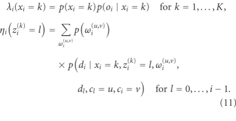
In this section we formulate the problem of data association in VSN with missing detections and show that it can be solved by inference on dynamic Bayesian networks. Suppose that K objects are moving in the region monitored byM
cameras, as shown in Figure 1. We use A = {auv}Mu,v=1 to
denote the parameter matrix of the VSN, each element of
Aconsists of three components, that is,auv =(πuv,tuv,suv),
a
b
c
d
e
f
g
h
i
j
Figure 1: Topology of visual sensor networks. Circles depict
cameras; edges depict path between cameras.
observations are collected to a data processing center and reordered according to their generating time, that is,di< dj ifi < jfor any two observationsyiandyj.
For each observation we introduce a labeling random variable xi ∈ {1,. . .,K}; xi = k indicates that the observation yi is originated from the objectk. In addition, we introduce another set of auxiliary random variableszi = {zi(k)}
K
k=1, eachz (k)
i ∈ {0,. . .,i−1} indicates which of the observations y0,. . .,yi−1 was the last observation of object k directly before the observation yi, and zi(k) = 0 means
yi is the first observation of object k. Both xi and zi are unobserved and considered as hidden states to be estimated based on available observations. The goal of data association is to calculate the marginal posterior distribution ofxi, that is, p(xi | y0:i). In this section we first define the state
transition model and observation model for the case of reliable detection and then introduce the routing random variables to accommodate the missing detections; finally we express the generating process of the observations sequence compactly with dynamic Bayesian networks.
3.1. State Transition Model. Based on the definition of hidden state variable xi and zi, it is reasonable to assume that the state evolve as a first-order Markov process. The state transition model can be written as
p(xi,zi|xi−1,zi−1)=p(xi)f
zi|xi−1=k,z(i−k)1=l
. (1)
The prior probability p(xi) can be assumed to follow a uniform distribution if no prior knowledge about xi is available. It should be noticed in above model that ifxi−1and zi−1are given, the value ofziis determined. Specifically, if the observation yi−1is produced by objectk, that is,xi−1 = k,
then z(ik) takes value of i−1 and other components in zi remain unchanged, that is,
z(ik)=z( k)
i−1[xi−1=/k] + (i−1)[xi−1=k], (2)
where [g]≡1(0) if and only if the logical variablegis true (false).
3.2. Observation Model. The observation includes appear-ance measurement and spatiotemporal measurement. We assume that they are conditionally independent given the current state, and both of them follow Gaussian distribution. The appearance observation model of a given object is
p(oi|xi=k)=N
oi;μk,σk2
, (3)
whereμkandσk2are mean and variance of the appearance of thekth object. The appearance observation is independent of the statezi. The spatiotemporal observation is dependent on
xi,ziand past observationsy0:i−1, as follows:
pdi,ci|xi=k, z(ik)=l,y0:i−1
=pdi|xi=k, zi(k)=l, dl,cl=u, ci=v
×pci=v|xi=k, zi(k)=l, dl,cl=u
=
⎧ ⎨ ⎩
c, l=0,
πuvN(di−dl;tuv,suv), l /=0.
(4)
Note that the spatiotemporal observation only depends on
zi(k)ifxi =k. As the observation y0is undefined, we set the
likelihood in the case ofl=0 to a constant valuec.
3.3. Missing Detection. At each monitoring camera, missing detection is unavoidable due to the unfavourable observing conditions. When the object of interest is miss detected, the true trajectory of that object cannot be expressed in terms of any sequence of state variablez(ik), i=1,. . .,N. This will introduce unpredictable errors in the likelihood evaluation according to (4) and hence deteriorate the performance of data association algorithm significantly. To deal with this problem, we introduce another set of random variable, namely, routing variablesωi = {ω(iu,v)}
M
u,v=1, to describe the
uncertainty in the object moving path. The routing variable
ω(iu,v)indicates the path with maximum length ofLtaken by an object moving from camerautov. It is a discrete random variable taking values in the set{1,. . .,RL
uv}, whereRLuvis the number of path form uto v not longer than L. The path length here is the number of camera nodes betweenuandv;
y0 y1 y2 y3
x1 x2 x3
Z1
1 z12 z13
z1K zK2 z3K
w1 w2 w3
. . .
. . .
. . .
(a)
wi
zi
xi
oi
di
ci
(b)
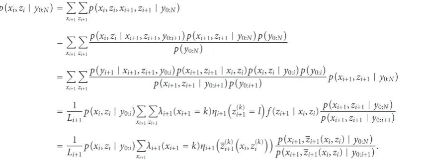
Figure2: (a): Dynamic Bayesian networks model; (b) dependency in a single time slice. Solid arrows depict stochastic dependency; dashed
arrows depicted deterministic one. Squares depict discrete random variables; circles depicted continuous ones.
p(xi−1|y0:i−1)
P(z(i−k)1|y0:i−1)
p(xi−1,z(i−k)1|y0:i−1)
p(xi−1,zi(−j)1,zi(−k)1|y0:i−1) p(xi,z (j) i ,z(
k) i |y0:i)
i−1 i
Belief state
Intermediate distributions
p(xi|y0:i)
p(z(ik)|y0:i)
p(xi,z(ik)|y0:i)
Figure3: Belief state propagation in forward pass ofApproximate
inferenceI. We only need to maintain the belief state the interme-diate distributions can be calculated based on the independence assumptions when necessary, as indicated by the arrows within each time slice.
p(xi−1|y0:i−1)
p(xi−1,z(i−k)1|y0:i−1)
p(xi−1,z(i−j)1,z (k)
i−1|y0:i−1) p(xi,z (j) i ,z(ik)|y0:i)
i−1 i
Belief state
Intermediate distributions
p(xi|y0:i)
p(xi,zi(k)|y0:i)
Figure4: Belief state propagation in forward pass ofApproximate
inferenceII. We only need to maintain the belief state the inter-mediate distributions can be calculated based on the independence assumptions when necessary, as indicated by the arrows within each time slice.
Treating (xi,zi,ωi) as hidden state, the state transition model can be written as
p(xi,zi,ωi|xi−1,zi−1,ωi−1)
=p(xi)p(ωi)fzi|xi−1=k,zi(−k)1=l
.
(5)
Note that zi is independent of ωi−1 given xi−1 and zi−1,
andxi,zi andωiare assumed to be mutually independent. When there is no observation to be conditioned on, the prior probability ofωiis determined by the topological structure of the camera networks. So it is reasonable to assume that the random variableωiis independent ofxiandzi. However,
whenωiis conditioned ony0:i, it is dependent onxiandzi through the spatiotemporal model (7). The prior probability of object moving path p(ωi) can be calculated according to the transition probabilities along that path. We useωi(u,v) = (u,w0(r),. . .,w
(r)
L−1,v) to denote therth path of lengthLfrom utov, wherew(r)is the intermediate nodes. Then the prior
probability of object taking therth path fromutovis
π(r)
uv p
ω(iu,v)=r
= πuw(0r)
L−1
l=1πwl(−r)1w (r)
l
πw(r)
L−1u
rπuw(0r)
L−1
l=1πwl(−r)1w (r)
l
πw(r)
L−1u
.
(6)
The spatiotemporal observation model changed to
p di,ci|xi=k, zi,ωi,y0:i−1
=pdi|xi=k,z(ik)=l, ωi(u,v)=r, dl,cl=u, ci=v
×pci=v|xi=k,z(ik)=l, ω
(u,v)
i =r, dl,cl=u
=
⎧ ⎪ ⎨ ⎪ ⎩
c, l=0,
Ndi−dl;tuv(r),s(uvr)
, l /=0.
(7)
Based on the Gaussian assumption, the mean and variance parameters in (7) can be calculated directly from the parameter matrixAof the VSN. The mean time of the object moving fromutovalong pathris
t(uvr)=tuw(0r)+
L−1
l=1 tw(r)
l−1w (r)
l +tw
(r)
L−1v. (8)
The variance of travelling time of the object moving fromu
tovalong pathris
s(r)
uv =suw0(r)+
L−1
l=1 sw(r)
l−1w (r)
l +sw
(r)
L−1v. (9)
RL
uv elements, and the rth element is composed of π(uvr),
t(uvr), and s(uvr). If the Gaussian assumption does not hold, the composite parameter matrix A cannot be constituted directly from A. In this case, A should be established manually. For example, if we assume that the traveling time between two directly connected cameras follows the log-normal distribution, which is useful for modeling the object’s long stay between cameras, the total traveling time along a specific path has no closed-form expression, but can be reasonably approximated by another log-normal distribution. A commonly used approximation is obtained by matching the mean and variance [23].
The model defined by (5)–(7) can be considered as a high-order probabilistic model in that it is capable of describing object’s transitions between nonadjacent nodes in the camera networks. The order of the model is determined by the path lengthL.
3.4. Graphical Representation. Dynamic Bayesian networks model probabilistic time series as a directed graph, where the nodes represent random variables and directed edges correspond to conditional probability distributions.Figure 2 shows the dynamic Bayesian networks model of the data association problem in VSN.
InFigure 2the arrows directed toziare defined by (2); the arrows directed to yi are defined by (3) and (7). To complete the model, we setz1(k)=0, fork=1,. . .,K.
4. Exact Inference
Based on the dynamic Bayesian networks model shown in Figure 2, data association problem in VSN can be solved by inferring the posterior marginal distribution of labeling variable p(xi | y0:i) from the observations and selecting the
label with the highest posterior probability. In this section we present the exact inference algorithms, including forward pass and backward pass, then show the intractability of the exact inference when the number of objects is large.
4.1. Forward Pass for Exact Inference. FromFigure 2we can see that ωi plays a role within a single time slice in DBN model, thus we define the belief state as the joint posterior probability of xi andzi and update it recursively based on the observation yi at each time instance. Having the state transition model and observation model in hand, this is a standard state estimation problem. From Bayesian rule, the forward pass belief state can be written as
p xi,zi|y0:i
=
ωi
p xi,zi,ωi|y0:i
= 1
Li
ωi
p yi|xi,zi,ωi,y0:i−1
p xi,zi,ωi|y0:i−1
= 1
Liλi(xi=k)ηi
z(ik)=l
p zi|y0:i−1
,
(10)
whereLi = p(yi | y0:i−1) is the normalizing constant. The
appearance and spatiotemporal information are injected into the model through the termsλiandηi, respectively, which are defined as follows:
λi(xi=k)=p(xi=k)p(oi|xi=k) fork=1,. . .,K,
ηi
z(ik)=l
=
ω(iu,v)
pω(iu,v)
×pdi|xi=k,z(ik)=l,ω
(u,v)
i ,
dl,cl=u,ci=v
forl=0,. . .,i−1.
(11)
Note that the probability items corresponding to all elements inωiexceptω(iu,v)are summed to one andω
(u,v)
i is completely encapsulated in the termηi. It turns out at this point that introducingωiresults in a mixed spatiotemporal observation model, as it can be expressed in terms of a weighted sum of probabilities conditioned on different paths. To calculate the predictive probability ofzi, we first calculate the predictive probability of the joint state (zi,xi−1) and then marginalize xi−1out. It can be written as
p zi,xi−1=j|y0:i−1
=
zi−1
f(zi|xi−1,zi−1)p xi−1=j,zi−1|y0:i−1
=
⎧ ⎪ ⎪ ⎪ ⎪ ⎪ ⎪ ⎪ ⎪ ⎪ ⎪ ⎪ ⎪ ⎪ ⎨ ⎪ ⎪ ⎪ ⎪ ⎪ ⎪ ⎪ ⎪ ⎪ ⎪ ⎪ ⎪ ⎪ ⎩
i−2
m=0
pxi−1=j,zi(−j)1=m,z (¬j)
i−1 =z (¬j)
i |y0:i−1
ifzi(j)=i−1,z
(¬j)
i =0,. . .,i−2,
otherwise
0,
(12)
wherez(i¬j)z
(1:K)
i \z
(j)
i . From the deterministic relationship of (2), ifxi−1 =j, the summands in the first line of (12) are
nonzero only whenzi(−¬1j)=z (¬j)
i . The last line of (12) ensures that allz(ik)cannot be less thani−1 simultaneously and only
zi(j)can be equal toi−1 ifxi−1= j.
p xi,zi|y0:N
=
xi+1
zi+1
p xi,zi,xi+1,zi+1|y0:N
=
xi+1
zi+1
p xi,zi|xi+1,zi+1,y0:i+1
p xi+1,zi+1|y0:N
p y0:N
p y0:N
=
xi+1
zi+1
p yi+1|xi+1,zi+1,y0:i
p(xi+1,zi+1|xi,zi)p xi,zi|y0:i
p y0:i
p xi+1,zi+1|y0:i+1
p y0:i+1
p xi+1,zi+1|y0:N
= 1
Li+1p x
i,zi|y0:i
xi+1
zi+1
λi+1(xi+1=k)ηi+1
z(i+1k)=l
f(zi+1|xi,zi)p xi+1
,zi+1|y0:N
p xi+1,zi+1|y0:i+1
= 1
Li+1p x
i,zi|y0:i
xi+1
λi+1(xi+1=k)ηi+1
z(i+1k)
xi,z(ik)
p xi+1,zi+1(xi,zi)|y0:N
p xi+1,zi+1(xi,zi)|y0:i+1
.
(13)
Note that the normalizing constant in (13) is already available andz(i+1k)is a function ofxiandz(ik), which is defined by (2).
Although the deterministic relation in (2) has simplified the inference computation significantly, it is clear in (10) and (13) that maintaining both forward and backward belief state is still intractable as the joint state space is the Cartesian product of the state space of xi and K spaces of all z(ik). At step i of forward passing, for example, there are KiK elements which need to be evaluated for updating the belief state. To make the inference practicable, we have to resort to approximate inference.
5. Approximate Inference
The basic idea of approximate inference is factorization. By factorizing the joint belief state into the product of several distributions of smaller sets of random variables, the memory and computational resources required for storing and updating belief state can be reduced. Inevitably, this factorization will introduce errors in belief state rep-resentation if the random variables in different sets are not indeed independent. However, Boyen and Koller [17] showed that, in terms of the Kullback-Leibler divergence, the inference error introduced by factorized representation of the belief state of discrete stochastic process is not accumulated infinitely over time. Furthermore, if the factorization is tailored to the specific structure of the process, the error has a bound determined by the minimum mixing rate of the involved subprocesses and the interaction among them. Theoretical results in [25] showed that using conditional independent clusters for approximate representation yields tighter bound. Although the theoretical results have not been extended to general stochastic process including continuous variables and to the case of reasoning backward in time, it is clearly suggested that for approximate inference, the structure of DBN may be exploited for computational gain in these circumstances. Following this line, in this section we present two kinds of factorization schemes based on the structure of DBN shown in Figure 2 and provide the
corresponding forward and backward algorithms. The effect of the algorithms is shown inSection 7with simulations and experiments.
The intractability of exact inference of our problem comes from the interdependency between variables. “Active path” [26] is a convenient tool for analyzing the dependence structure in belief networks: an active path from node i
to j given node set K is a simple trail between i and j, such that every node with two incoming arcs on the trail is or has a descendant in K and every other node on the trail is not functionally determined by K. Two nodes are interdependent if they are connected by an active path. In Figure 2we can identify the following two kinds of active paths: (a) active paths within a single time slice,zi(j)andz
(k)
i are coupled through the pathz(ij)−yi−zi(k), andxiandzi(k) are coupled throughxi−yi−zi(k); (b) active paths across the past time slices, and z(ij) andz
(k)
i are coupled through the pathsz(ij)−xi−1−z(ik) andz
(j)
i −z
(j)
i−1−yi−1−zi(−k)1−z (k)
i , and the longer paths z(ij) −z
(j)
i−1 −xi−2 −zi(−k)1 −z (k)
i and
zi(j)−z
(j)
i−1−z (j)
i−2−yi−2−z(i−k)2−z (k)
i−1−z (k)
i , and so on. It should be noticed, however, that the active paths betweenz(ik)s can be disconnected if the value ofxat proper time slice is given. For example,z(ij)−yi−zi(k)breaks ifxiis given; the pair of pathsz(ij)−xi−1−z(ik)andz
(j)
i −z
(j)
i−1−yi−1−z(i−k)1−z (k)
i break ifxi−1is given, and so on.
5.1. Approximate Inference I. In the first factorization scheme, the joint belief state is naively decomposed into the product of marginal distributions ofxiandzi(k), that is,
p xi,zi|y0:i
≈p xi,zi|y0:i
=p xi|y0:i
K
k=1
pzi(k)|y0:i
,
p xi,zi|y0:N
≈p xi,zi|y0:N
=p xi|y0:N
K
k=1
pz(ik)|y0:N
.
(14)
At stepi in the forward pass, the approximate belief state
p(xi−1,zi−1 | y0:i−1) is propagated through the transition
model, obtaining p(xi,zi | y0:i−1), and conditioned on
the current observation, obtaining p(xi,zi | y0:i), then
approximated by (14), obtainingp(xi,zi | y0:i). The process
of backward pass is similar.
5.1.1. Forward Pass in Approximate Inference I. To derive the forward pass algorithm, we first calculate the marginal distributions pi in (14) from (10) and then try to express them in terms of the marginal distributions of the last time instance pi−1 based on the independence assumption. The
marginal distribution ofxiis
p xi=k|y0:i
=
zi
p xi=k,zi|y0:i
= 1
Lif
λi(xi=k)
zi
ηi
zi(k)=l
p zi|y0:i−1
= 1
Lif
λi(xi=k)
z(ik)
ηi
zi(k)=l
pz(ik)=l|y0:i−1
.
(15)
Fork=1,. . .,K, the marginal distribution ofzi(k)is
pz(ik)=l|y0:i
=
xi
z(i¬k)
p xi,zi|y0:i
= 1
Lif
xi
z(i¬k)
λi(xi=k)ηi
z(ik)=l
p zi|y0:i−1
= 1
Lif
λi(xi=k)ηi
zi(k)=l
pz(ik)=l|y0:i−1
+ 1
Lif K
xi=1
xi=/ k
λi xi=j
z(ij)
ηi
z(ij)=m
×pz(ij)=m,z
(k)
i =l|y0:i−1
.
(16)
There are two kinds of predictive distributions in (15) and (16), one is over single z(ik), and the other is over the pair (z(ij),z
(k)
i ). We first calculate the joint predictive probabilities of them with xi−1, then marginalize xi−1 out. The joint
predictive distribution of (z(ik),xi−1) is
pz(ik)=l,xi−1=n|y0:i−1
=
z(i−k)1
fz(ik)=l|xi−1=n,z(i−k)1
pxi−1=n,zi(−k)1|y0:i−1 = ⎧ ⎪ ⎪ ⎪ ⎪ ⎪ ⎪ ⎪ ⎪ ⎨ ⎪ ⎪ ⎪ ⎪ ⎪ ⎪ ⎪ ⎪ ⎩
p xi−1=k|y0:i−1
ifn=k, l=i−1,
p xi−1=n|y0:i−1
×pzi(−k)1=l|y0:i−1
ifn /=k, l=0 :i−2,
otherwise 0.
(17)
The joint predictive distribution of (zi(k),z
(j)
i ,xi−1) is
pzi(j)=m,z(ik)=l,xi−1=n|y0:i−1
=
z(i−j)1
z(i−k)1
fzi(j)=m,z
(k)
i =l|xi−1=n,z(i−j)1,z (k)
i−1
×pxi−1=n,z(i−j)1,z (k)
i−1|y0:i−1 = ⎧ ⎪ ⎪ ⎪ ⎪ ⎪ ⎪ ⎪ ⎪ ⎪ ⎪ ⎪ ⎪ ⎪ ⎪ ⎪ ⎪ ⎪ ⎪ ⎪ ⎪ ⎪ ⎪ ⎪ ⎪ ⎪ ⎪ ⎪ ⎪ ⎪ ⎪ ⎪ ⎪ ⎪ ⎨ ⎪ ⎪ ⎪ ⎪ ⎪ ⎪ ⎪ ⎪ ⎪ ⎪ ⎪ ⎪ ⎪ ⎪ ⎪ ⎪ ⎪ ⎪ ⎪ ⎪ ⎪ ⎪ ⎪ ⎪ ⎪ ⎪ ⎪ ⎪ ⎪ ⎪ ⎪ ⎪ ⎪ ⎩
p xi−1=j|y0:i−1
pz(i−k)1=l|y0:i−1
ifn= j, m=i−1, l=0 :i−2,
p xi−1=k|y0:i−1
pz(i−j)1=m|y0:i−1
ifn=k, m=0 :i−2, l=i−1,
p xi−1=n|y0:i−1
pz(i−j)1=m|y0:i−1
×pzi(−k)1=l|y0:i−1
ifn /=j, n /=k, m=0 :i−2, l=0 :i−2,
otherwise
0.
(18)
5.1.2. Backward Pass in Approximate Inference I. The deriva-tion of backward pass algorithm is straightforward. We first substitute (14) into (13), obtaining
p xi,zi|y0:N
= 1
Lbi+1
p xi,zi|y0:i
×
xi+1
λi+1(xi+1=k)ηi+1
z(i+1k)
xi,zi(k)
× p xi+1,zi+1(xi,zi)|y0:N
p xi+1,zi+1(xi,zi)|y0:i+1
= 1
Lbi+1 p xi|y0:i
τ
pzi(τ)|y0:i
·
xi+1
λi+1(xi+1=k)ηi+1
z(i+1k)
xi,z(ik)
× p xi+1|y0:N
p xi+1|y0:i+1
τ
pz(i+1τ)
xi,z(iτ)
|y0:N
pz(i+1τ)
xi,z(iτ)
|y0:i+1
.
(19)
Note that in approximate inference the normalization con-stantLb
i+1=/ L
f
i+1. Then we calculate the marginal distribution
ofxi
p xi=n|y0:N
=
zi
p xi,zi|y0:N
= 1
Lbi+1
p xi=n|y0:i
×
xi+1
λi+1(xi+1=k)
τ
zi(τ)
η(i+1k)
xi,zi(τ)
φi+1
xi,z(iτ)
(20)
and the marginal distribution ofzi(k)
pz(ij)=m|y0:N
=
xi
zi(¬j)
p xi,zi|y0:N
= 1
Lb i+1
xi+1
λi+1(xi+1=k)
·
xi
p xi|y0:i
η(i+1k)
xi,zi(j)=m
φi+1
xi,z(ij)=m
×
τ /=j
zi(τ)
η(i+1k)
xi,z(iτ)
φi+1
xi,z(iτ)
,
(21)
p(xi=k|y0:N) Inference
Parameter estimation (αh,μk,σk)
Figure 5: The EM framework. The inference module is
imple-mented with the algorithms presented inSections 4and5, and the parameter estimation module is implemented with (34)–(36).
where the termsλi+1,η(i+1k), andφi+1are defined as
λi+1(xi+1=k)=λi+1(xi+1=k)
p xi+1|y0:N
p xi+1|y0:i+1
, (22)
η(i+1k)
xi=n,zi(τ)=l
= ⎧ ⎪ ⎪ ⎪ ⎪ ⎨ ⎪ ⎪ ⎪ ⎪ ⎩
1 ifτ /=k,
ηi+1
z(i+1k)=i
ifτ =k, n=k,
ηi+1
z(i+1k)=l
ifτ =k, n /=k,
(23)
φi+1
xi=n,z(iτ)=l
= ⎧ ⎪ ⎪ ⎪ ⎪ ⎪ ⎪ ⎪ ⎪ ⎨ ⎪ ⎪ ⎪ ⎪ ⎪ ⎪ ⎪ ⎪ ⎩
pzi(+1τ)=i|y0:N
pzi(+1τ)=i|y0:i+1
pzi(τ)=l|y0:i
ifn=τ,
pzi(+1τ)=l|y0:N
pzi(+1τ)=l|y0:i+1
pzi(τ)=l|y0:i
ifn /=τ.
(24)
5.2. Approximate Inference II. In the second factorization scheme, we preserve the interdependence betweenxiandzi and assume that zi(j) andz
(k)
i are conditional independent givenxi. Then the joint belief state is decomposed as
p xi,zi|y0:i
≈p xi,zi|y0:i
=p xi|y0:i
K
k=1 pz(k)
i |xi,y0:i
,
p xi,zi|y0:N
≈p xi,zi|y0:N
=p xi|y 0:N
K
k=1 pz(k)
i |xi,y0:N
.
(25)
The process of forward and backward pass is the same as before, except for the approximation manner of the belief state.
5.2.1. Forward Pass in Approximate Inference II. To write down the forward pass algorithm for belief state representa-tion in (25), we need to compute the marginal distriburepresenta-tions
poverxiand (xi,z(k)
(15), but with different definition of p(z(k)
i | y0:i−1). The
latter can be written as
pxi=j,z(k)
i =l|y0:i
=
z(i¬k)
pxi=j,z(k)
i =l,z(¬ k)
i |y0:i
= 1
Lif
λi xi=j z(i¬k)
ηi
z(ij)=m
p zi|y0:i−1
= ⎧ ⎪ ⎪ ⎪ ⎪ ⎪ ⎪ ⎪ ⎪ ⎪ ⎪ ⎪ ⎪ ⎨ ⎪ ⎪ ⎪ ⎪ ⎪ ⎪ ⎪ ⎪ ⎪ ⎪ ⎪ ⎪ ⎩ 1
Lif
λi(xi=k)ηi
z(ik)=l
×pz(k)
i =l|y0:i−1
if j=k,
1
Lif
λi xi=j
z(ij)
ηi
z(ij)=m
×pz(j)
i =m,z
(k)
i =l|y0:i−1
if j /=k.
(26)
Based on the independence assumption in (25), the two predictive distributions in (17) and (18) are redefined as
pz(k)
i =l,xi−1=n|y0:i−1
=
z(i−k)1
fz(ik)=l|xi−1=n,z(i−k)1
pxi−1=n,z(k)
i−1|y0:i−1 = ⎧ ⎪ ⎪ ⎪ ⎪ ⎨ ⎪ ⎪ ⎪ ⎪ ⎩
p x
i−1=k|y0:i−1
ifn=k, l=i−1,
px
i−1=n,zi(−k)1=l|y0:i−1
ifn /=k, l=0 :i−2,
otherwise 0,
(27)
pz(j)
i =m,z
(k)
i =l,xi−1=n|y0:i−1
=
z(i−j)1
zi(−k)1
fzi(j)=m,z
(k)
i =l|xi−1=n,z (j)
i−1,z (k)
i−1
×pxi−1=n,z(j)
i−1,z (k)
i−1|y0:i−1 = ⎧ ⎪ ⎪ ⎪ ⎪ ⎪ ⎪ ⎪ ⎪ ⎪ ⎪ ⎪ ⎪ ⎪ ⎪ ⎪ ⎪ ⎪ ⎪ ⎪ ⎪ ⎪ ⎪ ⎪ ⎪ ⎪ ⎪ ⎪ ⎪ ⎪ ⎪ ⎪ ⎨ ⎪ ⎪ ⎪ ⎪ ⎪ ⎪ ⎪ ⎪ ⎪ ⎪ ⎪ ⎪ ⎪ ⎪ ⎪ ⎪ ⎪ ⎪ ⎪ ⎪ ⎪ ⎪ ⎪ ⎪ ⎪ ⎪ ⎪ ⎪ ⎪ ⎪ ⎪ ⎩
pxi−1= j,z(k)
i−1=l|y0:i−1
ifn=j, m=i−1, l=0 :i−2,
pxi−1=k,z(j)
i−1=m|y0:i−1
ifn=k, m=0 :i−2, l=i−1,
pz(j)
i−1=m,xi−1=n|y0:i−1
p
p x
i−1=n|y0:i−1
×z(i−k)1=l,xi−1=n|y0:i−1
ifn /=j, n /=k, m=0 :i−2, l=0 :i−2,
otherwise
0.
(28)
When belief state is updated by (26)–(28) at step i, K +
K2i elements need to be evaluated. The forward pass
algorithm forapproximate inference IIis depicted graphically inFigure 4. Although the computational burden increases to some extent compared withapproximation inference I(but still much less than that in exact algorithm), simulation results show that the inference accuracy is improved signif-icantly, approaching that of the exact algorithm.
5.2.2. Backward Pass in Approximate Inference II. As before, to derive the backward pass algorithm for approximate inference II, we substitute (25) into (13), obtaining
p xi,zi|y
0:N
= 1
Lbi+1
p xi|y0:i
τ
pz(τ)
i |xi,y0:i
·
xi+1
λi+1(xi+1=k)ηi+1
z(i+1k)
xi,z(ik)
p x
i+1|y0:N
p x
i+1|y0:i+1
×
τ
pz(τ)
i+1
xi,zi(τ)
|xi+1,y0:N
pz(τ)
i+1
xi,zi(τ)
|xi+1,y0:i+1
,
(29)
then calculate the marginal distribution ofxi
p xi=n|y0:N
=
zi
p xi,zi|y0:N
= 1
Lb i+1
p xi=n|y
0:i
xi+1
λi+1(xi+1=k)
×
τ
zi(τ)
η(i+1k)
xi,zi(τ)
ψi+1
xi,zi(τ),xi+1
(30)
and the marginal distribution of (xi,zi(k))
pxi=n,z(j)
i =m|y0:N
=
zi(¬j)
p xi,zi|y0:N
= 1
Lbi+1
xi+1
λi+1(xi+1=k)η(i+1k)
xi,z(ij)
ψi+1
xi,zi(j),xi+1
×
τ /=j
z(iτ)
η(i+1k)
xi,z(iτ)
ψi+1
xi,zi(τ),xi+1
,
where λi+1, and η(i+1k) are defined by (22) and (23). ψi+1 is
defined as
ψi+1
xi=n,zi(τ)=l,xi+1=k = ⎧ ⎪ ⎪ ⎪ ⎪ ⎪ ⎪ ⎪ ⎪ ⎪ ⎪ ⎪ ⎪ ⎪ ⎪ ⎪ ⎪ ⎪ ⎪ ⎪ ⎪ ⎪ ⎪ ⎪ ⎪ ⎪ ⎪ ⎪ ⎪ ⎪ ⎪ ⎪ ⎪ ⎪ ⎪ ⎪ ⎪ ⎪ ⎨ ⎪ ⎪ ⎪ ⎪ ⎪ ⎪ ⎪ ⎪ ⎪ ⎪ ⎪ ⎪ ⎪ ⎪ ⎪ ⎪ ⎪ ⎪ ⎪ ⎪ ⎪ ⎪ ⎪ ⎪ ⎪ ⎪ ⎪ ⎪ ⎪ ⎪ ⎪ ⎪ ⎪ ⎪ ⎪ ⎪ ⎪ ⎩
pz(τ)
i+1=i,xi+1=k|y0:N
pz(τ)
i+1=i,xi+1=k|y0:i+1
·p xi+1=k|y0:i+1
p xi
+1=k|y0:N
·p
z(τ)
i =l,xi=n|y0:i
p xi=n|y0:i ifn=τ,
pz(τ)
i+1=l,xi+1=k|y0:N
pz(τ)
i+1=l,xi+1=k|y0:i+1
·p xi+1=k|y0:i+1
p xi+1=k|y0:N
·p
z(τ)
i =l,xi=n|y0:i
p x
i=n|y0:i
, ifn /=τ.
(32)
5.3. Discussion. In this section we will discuss the problem of choosing active path for approximate inference in more detail. Here we define the belief state as the joint distribution of (z1:K
i ,x1:i) and the exact forward inference can be
reformu-lated as
pzi1:K,x1:i|y0:i
= 1
Liλ
i(xi=k)ηi
z(ik)=l
×pz1:K i |x1:i−1
p x1:i−1|y0:i−1
= 1
Liλi(xi=k)ηi
z(ik)=l
× K
j=1
pz(ij)|x1:i−1
p x1:i−1|y0:i−1
,
(33)
where λi and ηi are defined in (11). Note that the joint predictive distribution of z1:K
i is completely decomposable given x1:i−1. In exact inference using (33), we have to
enumerate in the sampling space ofx1:i−1. This just shifts the
problem from the intractable enumeration ofz1:K
i to that of
x1:i−1. For tractable inference, we must discard some of the
conditioning variablesx1:i−1. Discarding allx1:i−1leads to the
proposed approximate inference II.
Formulation (33) provides a clearer view of the “relative significance” of active path corresponding to variable xτ,
τ = 1 : i−1. Note that with some probability δτ, z(ij) is functionally determined by xτ. In other words, the τth active path is disconnected byxτ with probabilityδτ. Thus we can use δτ as a measure of the “relative significance” of theτth active paths. It is easy to show thatδτ decreases exponentially as τ varying from i − 1 to 1. In fact, for time slice i, the relative significance of i − 1th path is
0 5 10 15 20 25 30 35 40
0 2 4
(a)
0 5 10 15 20 25 30 35 40
0 2 4
(b)
0 5 10 15 20 25 30 35 40
0 2 4
(c)
0 5 10 15 20 25 30 35 40
0 2 4
(d)
Figure 6: Marginal distribution of labeling variable in exact
inference. The 24th and 34th observations are missed, depicted as dashed column. The true labels are depicted by stars. Each column represents the marginal distribution of the label of an observation. Grayscale corresponds to probability value. Black represents probability 1 and white probability 0. (a) Forward pass with 0-order model. (b) Forward pass with 1-order model. (c) Backward pass with 0-order model. (d) Backward pass with 1-order model.
δi−1 = p(xi−1 = j), and the relative significance ofi−2th
path isδi−2=p(xi−1=/ j)p(xi−2=j), and so on (we omit the
conditioning variablesy0:i−1temporally for clarity). This fact
implies that the “recent” active paths are far more important than the “ancient” ones for accurate inference as they are less likely to be disconnected. We delete the conditioning variablesxτin (33) one by one fromτ=1 toi−1, resulting in a set of approximate inference algorithms and compare them with the proposed approximate inference II. We observed in simulations that the conditioning variables xτ earlier than
i−1 have much less effect on inference accuracy thanxi−1
and includingxi−1can only improve the inference accuracy
to a limited extent, but at the cost of a significant increase in computational burden.
0 5 10 15 20 25 30 35 40 0
2 4
(a)
0 5 10 15 20 25 30 35 40
0 2 4
(b)
0 5 10 15 20 25 30 35 40
0 2 4
(c)
0 5 10 15 20 25 30 35 40
0 2 4
(d)
0 5 10 15 20 25 30 35 40
0 2 4
(e)
0 5 10 15 20 25 30 35 40
0 2 4
(f)
Figure7: Marginal distribution of labeling variable in exact inference. The 3rd, 8th, 13th, 28th, 32nd, and 33rd observations are missed,
depicted as dashed column. The true labels are depicted by stars. Each column represents the marginal distribution of the label of an observation. Grayscale corresponds to probability value. Blacks represent probability 1 and white probability 0. (a) Forward pass with 0-order model. (b) Forward pass with 1-0-order model. (c) Forward pass with 2-0-order model. (d) Backward pass with 0-0-order model. (e) Backward pass with 1-order model. (f) Backward pass with 2-order model.
independence, which is just the same scheme used in our approximate inference II. The authors in [27] point out that the more conditioning variables preserved, the tighter the bound is. This is also consistent with our results. However, it is not clear in [27] how to choose the conditioning variables in an optimal way. Besides, our approximate inference (I and II) is similar with the Factored Frontier algorithm [28] in that both of them factorize the joint belief state. But there is one important difference: our algorithms update the factored belief state from time t − 1 to t exactly before computing the marginals in t, whereas Factored Frontier computes the approximate marginals directly based on additional independence assumption, resulting in more errors in calculation.
It is tempting in application that the independence structure can be discovered automatically. This enables the algorithm to choose the approximation scheme adaptively according to changing situations. We notice that in [29] an incremental thin junction tree algorithm is proposed which can adaptively choose a set of clusters and separators, that is, a junction tree, at each time step to approximate the belief state. We plan to incorporate this idea into our method in the future.
6. EM Framework for Unknown
Appearance Parameters
In the previous discussion, we assumed that the appearance models of the objects under tracking are available. However, in typical scenarios of practical interests, the parameters of the appearance model are usually unknown and need to be estimated from observations. If we had known the label of each observation, that is, the object from which the observation is generated, the parameter estimation is straightforward. But the labels are also unknown and need to be estimated with data association algorithms. Considering the hidden labels as missing data, the problems of parameter
estimation and data association can be solved simultaneously under the EM framework [30].
In this paper, the appearance observations are assumed to be generated from Gaussian mixture model, and the E-step and M-E-step in the EM framework take a very intuitive and simple form. We use Θ = {αk,μk,σk}Kk=1 to denote the model parameters, where αk p(xi = k) is the prior probability of the label k, μk and σk are mean and variance of appearance of object k. In E-step, based on the old guess of the model parameters Θold, we calculate
the ownership probability of each observation, that is, the posterior probability of the hidden label corresponding to each observation,p(xi|y0:N,Θold), with the data association algorithm presented in previous sections. Note that if we use forward passing algorithm for inference, the ownership probability is p(xi|y0:i,Θold). In M-step, the model
param-eters are updated as in classical EM algorithm for Gaussian mixture model [31]
αnewk = 1
N
N
i=1
pxi=k|y0:N,Θold
,
μnew
k =
N
i=1oip xi=k|y0:N,Θold
N
i=1p xi=k|y0:N,Θold
,
σknew=
N
i=1p xi=k|y0:N,Θold
oi−μnewk
oi−μnewk
N
i=1p xi=k|y0:N,Θold
.
(34)
0 100 200 300 400 500 600 700 800 900 1000 fwd approximate I
0 1 2 3 4 5 6
(a)
0 100 200 300 400 500 600 700 800 900 1000 bwd approximate I
0 2 4 6 8 10 12
(b)
0 100 200 300 400 500 600 700 800 900 1000 fwd approximate II
0 0.2 0.4 0.6 0.8 1 1.2 1.4
(c)
0 100 200 300 400 500 600 700 800 900 1000 bwd approximate II
0 0.5 1 1.5 2 2.5
(d)
0 100 200 300 400 500 600 700 800 900 1000 fwd
10−20 10−15 10−10 10−5 100 105
Approximate I Approximate II
(e)
0 100 200 300 400 500 600 700 800 900 1000 bwd
10−16 10−14 10−12 10−10 10−8 10−6 10−4 10−2 100 102
Approximate I Approximate II
(f)
Figure8: KL divergence caused by approximate inference. (a) Forward approximate I. (b) Backward approximate I. (c) Forward approximate
II. (d) Backward approximate II. (e) Comparison between smoothed KL divergence of forward approximates I and II in log domain. (f) Comparison between smoothed KL divergence of backward approximates I and II in log domain.
model can be used for online data association using forward inference algorithms. In the future, we plan to investigate how to incorporate the inference engine into online EM such that both model learning and data association can be accomplished simultaneously on the fly. It is interested if we could estimate the parameters in the spatiotemporal model using EM as well. However, in M step, it is difficult to find an algorithm similar to (34) to update the guessed value of spatiotemporal parameters due to the existence of missing detections.
7. Results
7.1. Simulations
7.1.1. Data. To generate simulation data, we use the VSN with topological model shown as Figure 1and specify the parameter matrix A of VSN and the appearance model parameters (μk,σ2
0 0.5 1 1.5 2 2.5 3
fwd exact
Appearance noise
fwd approximate I fwd approximate II 60
65 70 75
M
at
ching
ac
cur
acy
(%)
80 85 90 95 100
(a)
0 0.5 1 1.5 2 2.5 3
bwd exact
Appearance noise bwd approximate I
bwd approximate II 30
40 50 60
M
at
ching
ac
cur
acy
(%)
70 80 90 100
(b)
Figure9: Mean accuracy under different appearance noise level.X-axis corresponds to the variance of appearance observations. (a) Forward
inference. (b) Backward inference.
0.1 0.2 0.3 0.4 0.5 0.6 0.7
fwd exact
Traveling time noise
fwd approximate I fwd approximate II 0
20 40
M
at
ching
ac
cur
acy
(%)
60 80 100
(a)
0.1 0.2 0.3 0.4 0.5 0.6 0.7
bwd exact
Traveling time noise
bwd approximate I bwd approximate II 0
20 40
M
at
ching
ac
cur
acy
(%)
60 80 100
(b)
Figure10: Mean accuracy under different level of traveling time standard deviation.X-axis corresponds to the ratio of standard deviation
to mean value of the traveling time observations. (a) Forward inference. (b) Backward inference.
the standard deviation of travel time is assumed to be proportional to its mean value. In each simulation, for the kth object, we choose its starting node randomly in Figure 1, then generate its moving trajectory according to the transition probabilities πuv. On each node along the trajectory of thekth object, the spatiotemporal observations
di and appearance observations oi are drawn from the assumed Gaussian model. We assume that at each time instance, there is only one object being observed by a camera. The observations of all objects are collected together and reordered according to the time observation, resulting in the data set{yi}.
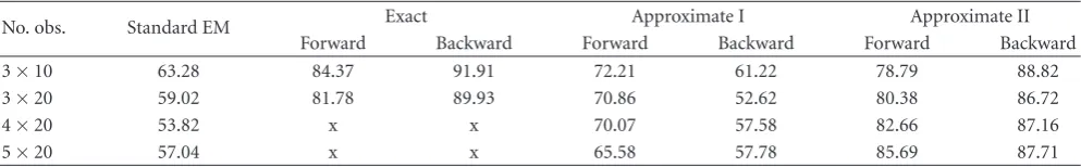
7.1.2. Evaluation Criteria. The criterion we use is the data associationaccuracy, denoted asq:
q= 1 K
K
k=1
qk qk=
Yk∩Yk
|Yk| ·
100%, (35)