Volume 2006, Article ID 83727, Pages1–16 DOI 10.1155/ASP/2006/83727
An Analysis of ISAR Image Distortion Based
on the Phase Modulation Effect
S. K. Wong, E. Riseborough, and G. Duff
Defence R&D Canada - Ottawa, 3701 Carling Avenue, Ottawa, ON, Canada K1A 0Z4
Received 28 April 2005; Revised 26 August 2005; Accepted 16 December 2005
Distortion in the ISAR image of a target is a result of nonuniform rotational motion of the target during the imaging period. In many of the measured ISAR images from moving targets, such as those from in-flight aircraft, the distortion can be quite severe. Often, the image integration time is only a few seconds in duration and the target’s rotational displacement is only a few degrees. The conventional quadratic phase distortion effect is not adequate in explaining the severe blurring in many of these observations. A numerical model based on a time-varying target rotation rate has been developed to quantify the distortion in the ISAR image. It has successfully modelled the severe distortion observed; the model’s simulated results are validated by experimental data. Results from the analysis indicate that the severe distortion is attributed to the phase modulation effect where a time-varying Doppler frequency provides the smearing mechanism. For target identification applications, an efficient method on refocusing distorted ISAR images based on time-frequency analysis has also been developed based on the insights obtained from the results of the numerical modelling and experimental investigation conducted in this study.
Copyright © 2006 Hindawi Publishing Corporation. All rights reserved.
1. INTRODUCTION
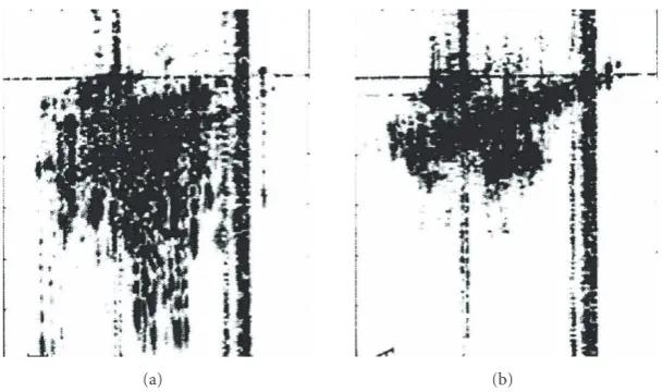
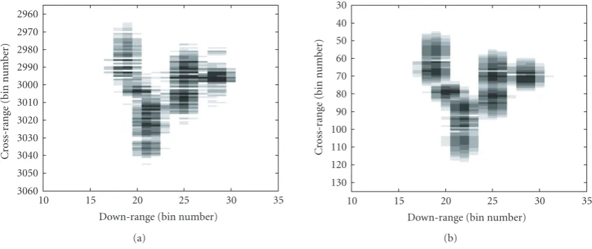
Inverse synthetic aperture radar (ISAR) imaging provides a 2-dimensional radar image of a target. A 2-dimensional picture can potentially offer crucial information about the features of the target and provide improved discrimination, leading to more accurate target identification. An ISAR im-age of a target is generated as a resul of the target’s rotational motion. This motion can sometimes be quite complex, such as that of a fast, manoeuvring jet aircraft. As a result, severe distortion can occur in the ISAR image of the target [1]. An illustration of a distorted ISAR image of an aircraft is shown inFigure 1(a); it can be seen clearly that the ISAR image is severely blurred. It has been recognized that a time-varying rotating motion from the rotation of the target is respon-sible for the image blurring [2]. Figure 2(a) shows the az-imuth angular displacements of the aircraft inFigure 1(a)as a function of time, as recorded independently by a ground-truth instrument mounted on-board the aircraft. When the target’s rotation is relatively smooth (Figure 2(b)), the mea-sured ISAR image of the aircraft is relatively well focused; this is illustrated inFigure 1(b). In addition, the temporal phase histories of a scattering centre on the aircraft from both the blurred and focused ISAR images also display the same tem-poral behaviour as the rotating azimuth motion of the air-craft; this is illustrated in Figures2(c)and2(d), respectively.
It is clearly seen that there is a direct correspondence between the distortion in the ISAR image and the nonuniform rota-tional motion of the target.
Although the distortion in ISAR images has been recog-nized as due to the higher-order Doppler motion effect from the target’s rotation [3], much of the analysis on ISAR dis-tortion is focused on the second-order effect of the target’s rotational motion [2,3] and the distortion is conventionally attributed to the quadratic phase effect [4,5]. This quadratic phase error is a result of a constant circular motion of the target with respect to the radar, resulting in a nonconstant Doppler velocity introduced along the radar’s line of sight due to the acceleration of the target from the circular mo-tion [4]. Quadratic phase distortion is significant only when the target image is integrated over a large angular rotation by the target and it does not provide an adequate account of the severe blurring in many of the observed ISAR images from real targets. Furthermore, time-frequency analysis of the dis-torted ISAR images often reveals that the motion of the target is fluctuating randomly and displays no temporal quadratic phase behaviour.
(a) (b)
Figure1: Example of (a) a distorted ISAR image and (b) an undistorted ISAR image of an in-flight aircraft [1].
250 200 150 100 50
0
Time (HRR pulse number) 0
0.5 1 1.5 2 2.5 3
R
elati
ve
azim
uth
ang
le
(deg
re
es)
(a)
250 200 150
100 50
0
Time (HRR pulse number) 0
0.5 1 1.5 2 2.5
R
elati
ve
azim
uth
ang
le
(deg
re
es)
(b)
250 200 150
100 50
0
Time (HRR pulse number) 0
20 40 60 80 100 120 140 160
R
elati
ve
phase
(ar
b
.unit)
(c)
250 200 150 100 50
0
Time (HRR pulse number) 0
10 20 30 40 50 60 70 80
R
elati
ve
phase
(ar
b
.unit)
(d)
distorting mechanism. This model includes many higher-order terms in the Doppler motion beyond the quadratic term in the phase of the target echo that some of the cur-rent analysis employed [2–6]. Experiments are conducted to study and to demonstrate the severe distortion in ISAR im-ages. The measured data are used for comparing and vali-dating the model’s simulated results. The comparative results indicate that the model provides an accurate account of the ISAR distortion. The distortion can be attributed to a mod-ulation effect in the phase of the target echo as a result of a time-varying Doppler motion of the target. It will also be shown that the quadratic phase distortion may be seen as a special case of the phase modulation effect; however, it can-not account for the severe distortion as observed in measured data.
For target recognition applications, a blurred ISAR image has to be refocused so that it can be used for target identifi-cation. Time-frequency signal processing techniques can be applied to effectively refocus distorted ISAR images [6]. In time-frequency processing, an ISAR image of a target is ex-tracted from a short-time interval; a focused image is thus obtained because the target’s motion can be considered as relatively uniform over a short duration. However, there are a large number of subintervals to deal with in the refocus-ing processrefocus-ing. It is very time-consumrefocus-ing to examine all re-focused ISAR images to search for the best image. An effi -cient ISAR refocusing procedure is developed to extract an optimum refocused image quickly without having to process a large number of images systematically. Issues such as how to locate the appropriate time instant to extract the best refo-cused image [7] and how to determine the appropriate time window width [8] will also be discussed.
2. ISAR IMAGING OF A MOVING TARGET
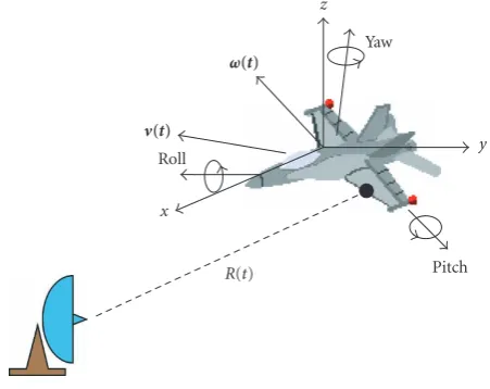
In general, a moving target could possess pitch, roll, and yaw motions simultaneously, in addition to a translational mo-tion at any given instant of time. These momo-tions all con-tribute to a resultant rotation of the target with respect to the radar that defines the formation of an ISAR image of the target. For a target with an arbitrary orientation relative to the radar, the various motions of the target are depicted in Figure 3. The phase in the radar echo of a scatter on the tar-get is given by
φ=4π f
c R(t), (1)
whereR(t) is the line-of-sight distance between the scatterer and the radar. Since the radar can detect a target’s motion along the radar’s line of sight only, it is therefore logical to define a target coordinate reference system in which thex -axis is parallel to the radar’s line of sight; this is illustrated inFigure 3. The changes inR(t) during the imaging interval can be expressed in terms of the target’s motion parameters as
R(t)=R0− t
0
v(τ)·xdτ−
t
0
ω(τ)×r(τ)·xdτ, (2)
Roll
Pitch Yaw
x
y z
v(t)
ω(t)
R(t)
Figure3: Various motions possessed by a moving target.
whereR0is the initial distance between the scatterer and the radar at the beginning of the imaging scan. The second term is the radial displacement of the scatterer due to the trans-lational motion of the target;v is the translational velocity vector and xdenotes the unit directional vector parallel to the radar’s line of sight. The third term is the line-of-sight displacement of the scatterer as a result of the rotational mo-tion of the target;ωis the rotational vector from the resultant angular motion of the target andris the positional vector of the scatterer on the target measured from the intersection of
ωand thex-axis (seeFigure 4). The rotational motion of the target provides a Doppler frequency shift that allows the scat-terer to be imaged along the cross-range of the ISAR image. The Doppler frequency at timetis given by
fD= 4π f
c
ω(t)×r(t)·x, (3)
where f is the radar frequency. The resultant rotational vec-torωincludes the pitch, roll, and yaw motions, as well as any relative rotation as a result of the translational motion of the target relative to the radar. As an example, an aircraft flying across in front of the radar from one side to the other will produce an apparent yaw motion of the target as seen by the radar tracking the movement of the aircraft. The rotational displacement of a scatterer on the target
X(t)=
t
0
ω(τ)×rτ)dτ (4)
provides the Doppler motion information on the phase of the radar echo for the ISAR image processing.
x
y z
(x,y,z)
ωx ωy
ωz
ϕ
θ
ω(t)
R(t)
r
Figure4: A Cartesian coordinate reference frame for the target with respect to the radar. Thex-axis is aligned parallel to the radar’s line of sight.
rewritten as
X(t)=
t
0
ω(τ)×r(τ)dτ=
t
0vR(τ)dτ= t
0
dxR(τ)
dτ dτ
=
xt
x0dxR=
x(t)−x0
x+y(t)−y0
y+z(t)−z0
z
(5)
for a general arbitrary rotation in which a scatterer on the target moves from coordinates (x0,y0,z0) att0=0 to a new position at (x,y,z) at timetduring a small time intervalΔt=
t−t0andx,y,zare the unit directional vectors. Moreover,
the rotational vectorωof the target can be decomposed into three orthogonal components; that is,
ω(t)=ωx(t)x+ωy(t)y+ωz(t)z. (6)
This is shown inFigure 4, andωx(t),ωy(t), and ωz(t) are the amplitudes of the three orthogonal rotating components (rad/s). It is intuitively obvious fromFigure 4that only the rotational components rotating about thez-axis (ωzz) and rotating about the y-axis (ωyy) of the target will have con-tribution to the displacement along thex-axis (i.e., along the radar’s line of sight). The change in the position of the scat-terer as a result of a rotation about thez-axis is given by
⎛ ⎜ ⎜ ⎝ x y z ⎞ ⎟ ⎟ ⎠= ⎛ ⎜ ⎜ ⎝
cos(Δθ) −sin(Δθ) 0 sin(Δθ) cos(Δθ) 0
0 0 1
⎞ ⎟ ⎟ ⎠ ⎛ ⎜ ⎜ ⎝ x0 y0 z0 ⎞ ⎟ ⎟
⎠, (7)
whereΔθ=ωzΔtis the amount of rotation parallel to thex
-yplane. This is the rotational motion that causes a change in the azimuth of the target as seen from the radar’s perspective. The change in the position of the scatterer rotating about the
y-axis is given by ⎛ ⎜ ⎜ ⎝ x y z ⎞ ⎟ ⎟ ⎠= ⎛ ⎜ ⎜ ⎝
cos(Δϕ) 0 sin(Δϕ)
0 1 0
−sin(Δϕ) 0 cos(Δϕ) ⎞ ⎟ ⎟ ⎠ ⎛ ⎜ ⎜ ⎝ x0 y0 z0 ⎞ ⎟ ⎟
⎠, (8)
whereΔϕ = ωyΔtis the amount of rotation about the y -axis. This is the rotational motion that causes a change in the elevation of the target as seen by the radar. The combined resultant displacement can be expressed as
⎛ ⎜ ⎝ x y z ⎞ ⎟ ⎠= ⎛ ⎜ ⎝
cos(Δϕ) 0 sin(Δϕ)
0 1 0
−sin(Δϕ) 0 cos(Δϕ) ⎞ ⎟ ⎠ ⎛ ⎜ ⎝
cos(Δθ) −sin(Δθ) 0 sin(Δθ) cos(Δθ) 0
0 0 1
⎞ ⎟ ⎠ ⎛ ⎜ ⎝ x0 y0 z0 ⎞ ⎟ ⎠ = ⎛ ⎜ ⎝
cos(Δθ) cos(Δϕ) −sin(Δθ) cos(Δϕ) sin(Δϕ) sin(Δθ) cos(Δθ) 0
−cos(Δθ) sin(Δϕ) sin(Δθ) sin(Δϕ) cos(Δϕ) ⎞ ⎟ ⎠ ⎛ ⎜ ⎝ x0 y0 z0 ⎞ ⎟ ⎠. (9)
Hence, the displacement of a scatterer along the x-axis is given by
X=x−x0=
x0
cos(Δθ) cos(Δϕ)
−y0
sin(Δθ) cos(Δϕ)+z0sin(Δϕ)
−x0. (10)
This is a somewhat complex expression to keep track of in a numerical analysis and too complex to be used in a
Radar line of sight
x y
(0,y0)
(x0, 0) ω
Figure5: Schematic of a rotating target with examples of two scat-tering centres illustrated. The target is rotating about thez-axis (out of page).
2-dimensional target with scatterers located on thex-yplane parallel to the line of sight, rotating about thez-axis; this is illustrated inFigure 5. It should be emphasized that the sim-plification of the target geometry does not alter the physics of the problem; rather, it offers a clearer physical insight of the problem by removing the unnecessary clutters in the algebra.
3. ISAR DISTORTION MODEL
In order to bring out the basic ISAR distortion mechanism more clearly, we will consider just one scatterer on the tar-get in the following analysis. This allows us to illustrate the physics analytically without any loss of generality. From (1) and (2), the phase of the radar return signal from a scatterer on a moving target is given by
φ=4π f
c
R0−vt−X(t)
, (11)
where f is the transmitting radar frequency,R0is the initial distance of the scatterer on the target from the radar at the onset of the radar imaging scan,vis the radial velocity of the scatterer, andX(t) is the displacement due to the rotation of the scatterer along the radar’s line of sight. Using the target geometry as shown inFigure 5, a change in the scatterer’s co-ordinates due to a rotation about thez-axis at a later timet
can be expressed succinctly as
x(t)
y(t)
=
cosω(t)t −sinω(t)t
sinω(t)t cosω(t)t x0
y0
(12)
according to (7). The displacement along the radar’s line of sightX(t)=x(t)−x0due to a rotation of the target is then given by
X(t)=x0cos
ω(t)t−y0sin
ω(t)t−x0. (13) Thus anX(t) due to a time-varying rotational motion dur-ing the ISAR imagdur-ing period can be modelled by a series of small displacements using (13) to cover the whole imaging duration. Note that the rotational rate in (13) is expressed as a function of time; that is,ω(t). A time-varying rotational rate can be fitted, in general, by a Fourier series; that is,
ω(t)≈ω0+
∞
n=1
ancos
nπt T
+bnsin
nπt T
, (14)
whereω0is the constant rotational rate of the target in the ab-sence of any extraneous fluctuation in the rotational motion,
T is the ISAR imaging period andan,bncan be considered as random variables for fittingω(t) to any fluctuating mo-tion during the imaging period, 0 ≤t ≤ T. Note that it is customary to use the symbol≈in the Fourier series equation (14) to indicate that the series on the right-hand side may not necessarily converge exactly toω(t).
An ISAR image is generated using a sequence of high range resolution (HRR) profiles. Firstly, detected target echoes are demodulated and converted into digitized in-phase and quadrature (I,Q) signals in the frequency domain. Then, the HRR profile of a scatterer can be generated by ap-plying a discrete Fourier transform to the frequency-domain in-phase and quadrature signal data [9],
Hn= N−1
i=0
(I+jQ)iexp
j2π Nni
=hnexp
j4π fc c
R0−vt−X(t)
exp
jN−1 N πn
,
(15)
where hn is the amplitude of the HRR profile with a sin(Nx)/sin(x) envelop, n is the range-bin index, n =
0,. . .,N −1; fc is the centre frequency of the radar band-width, andR0andX(t) are defined in (11). A second discrete Fourier transform is then performed at each of the range bins over the sequence of HRR profiles to generate an ISAR image; that is,
In,m= M−1
k=0
hn,kexp
j4π fc c
R0−vt−X(t)
×exp
jN−1 N πn
exp
j2π Mmk
,
(16)
where mis the cross-range bin index, m = 0,. . .,M−1.
Mis the number of HRR profiles used in the generation of the ISAR image. The radial target motion is assumed to be compensated; that is,vtis set to zero. In effect, the second Fourier transform converts the HRR variable at each range bin from the time domain into the frequency domain. Hence, the cross-range dimension of the ISAR image represents the Doppler frequency as observed by the radar. The term that is of interest in the analysis of the distortion in an ISAR image is the phase factor containing the temporal rotational displace-mentX(t) in (16); that is,
ψ(t)=exp
−j4π fc c X(t)
=exp
−j4π fc c
x0cos
ω(t)t−y0sin
ω(t)t−x0
.
(17)
Equation (17) forms the basis of the numerical model for computing the ISAR distortion of a target due to a time-varying rotational motion.
analytically. This would give us a better physical insight of the problem. To derive an analytical expression for the distortion mechanism, the phase factor due to rotation is rewritten as
ψ(t)=exp
−j4π fc c X(t)
=exp
−j4π fc c
t
0
ω(τ)×r(τ)·xdτ
=exp
−j4π fc c
t
0
ω(τ)r(τ)sinθ dτ (18)
by substituting (4) forX(t). Then, consider a short-time in-stant when the scatterer is located at (0,y0) where the scat-terer’s motion is parallel to the radar’s line of sight (see Figure 5); this corresponds to the largest Doppler effect as seen by the radar. To obtain an analytical expression, two simplifying steps are taken. First, a simplified time-varying rotational rate is assumed and is given by
ω(t)=ω0+ωrsin(2πΩt), (19)
whereω0is a constant,ωris the rotational amplitude of the fluctuating motion, andΩis the fluctuating frequency of the time-varying motion. A second simplifying step is to assume that the distance between the scatterer at (0,y0) and the ro-tation centre of the target is more or less constant such that
r(t) ≈ y0during this time instant as depicted inFigure 5. This assumption is a reasonable one because normally, the ISAR image of a target is captured during a relatively small rotation of the target. For example, the ISAR images gen-erated inFigure 1correspond to a rotation of only about 3 degrees; hencer(t)is nearly constant. Furthermore, sinθ
is set to−1 (in (18)), corresponding toθ = −90 degrees as measured from thex-axis inFigure 5; this is consistent with the target geometry shown inFigure 5 where the scatterer at (0,y0) has the maximum Doppler velocity and is moving away from the radar. Applying these 2 simplifying assump-tions and substituting (19) into (18),
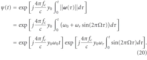
ψ(t)=exp
j4π fc c y0
t
0
ω(τ)dτ
=exp
j4π fc c y0
t
0
ω0+ωrsin(2πΩτ)
dτ
=exp
j4π fc c y0ω0t
exp
j4π fc c y0ωr
t
0sin(2πΩτ)dτ
.
(20)
The first factor in (20) corresponds to a constant rotation of the target. This factor provides a Doppler shift that allows the scatterer to be imaged along the cross-range dimension to form an undistorted ISAR image of the target in the ab-sence of any fluctuating motion. The second factor describes a phase modulation effect due to a temporally fluctuating motion of the scatterer that introduces distortion in the ISAR image. To see how the phase modulation effect comes about more clearly, the second phase factor in (20) can be rewritten
as
μ(t)=exp
j4π fc c y0ωr
t
0sin(2πΩτ)dτ
=expjksin(η)
=cosksin(η)+jsinksin(η)
=J0(k) + 2J2(k) cos(2η) + 2J4(k) cos(4η) +· · ·
+j2J1(k) sin(η) + 2J3(k) sin(3η) + 2J5(k) sin(5η) +· · ·,
(21)
where
k=4π fc
c y0, η=sin−1
ωr t
0sin(2πΩτ)dτ
,
(22)
and theJnare the Bessel functions of the first kind of ordern. It can be seen from (21) that the phase of a time-dependent rotational motion consists of many higher-order sideband components. These higher-order sideband components are a consequence of phase modulation from a temporally fluc-tuating target motion and they have been shown to produce a smear in the radar image as a result [10].
4. ISAR DISTORTION EXPERIMENTS
An ISAR experiment is set up to examine the distortion in ISAR images due to a time-varying rotational motion. There are a number of reasons why data from a controlled experi-ment are desirable. In a controlled experiexperi-ment, the locations of the scattering centres and the rotational axis of the tar-get are known precisely. The rotational motion of the tartar-get can be programmed and controlled to produce the desired effects that are sought for analysis. Moreover, experiments of a given set of conditions can be repeated to verify the consis-tency of the results. These are not always possible with real targets such as in-flight aircraft. Data from controlled exper-iments can then be used to compare with simulated results from the numerical model under the same set of conditions. Such comparison provides a meaningful validation of the nu-merical model, thus providing a clearer picture of the distort-ing process.
Figure6: The target motion simulator (TMS) experimental appa-ratus.
ω
Figure7: Schematic of the ISAR imaging experimental setup.
experimental setup; note that one corner reflector is placed asymmetrically to provide a relative geometric reference of the TMS target. A time-varying rotational motion is intro-duced by a programmable motor drive. ISAR images of the TMS target are collected atX-band from 8.9 GHz to 9.4 GHz using a stepped frequency radar waveform with a frequency step size of 10 MHz and a radar repetition rate PRF=2 kHz. A sequence of ISAR images of the TMS apparatus is shown inFigure 8, corresponding to the target making a transition from a constant rotation (Figure 8(a)) to a time-varying ro-tational motion (Figures8(b)and8(c)).Figure 8(a)shows an ISAR image that is well focused with the 6 reflectors shown clearly; the target is rotating with a constant motion of about 2.0 degrees/s. A fluctuating motion is then added to the mo-tion of the target. The ISAR images become distorted as seen in Figures8(b)and8(c). The actual fluctuating target motion that corresponds to the distortion inFigure 8(c)is shown in Figure 9(a); the motion is extracted from the experimental ISAR image as a time-frequency spectrogram [9]. The rota-tional displacement of the target is shown inFigure 9(b). The target has rotated 8 degrees during a 4-second imaging inter-val. The fluctuating motion is clearly evident from the rip-pling behaviour of the rotational displacement of the target inFigure 9(b). It is also evident that the fluctuating rotational motion deviates less than 1 degree from a smooth uniform rotating motion (dashed line in Figure 9(b)) at any given instant of time during the imaging interval. This serves to
illustrate that even though the amount of perturbed motion on the target is very small, the amount of distortion intro-duced in the ISAR image of the target can be quite signifi-cant as shown inFigure 8(c). This result is consistent with the severe distortion observed from a real target as shown in Figure 1(a).
5. ISAR DISTORTION ANALYSIS
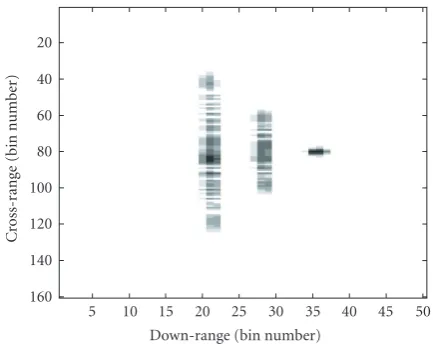
A distorted ISAR image of the TMS target computed by the numerical model based on (17) is shown in Figure 10; the computation is done using the experimental parameters as inputs. It can be seen fromFigure 10that the computed dis-tortion in the ISAR image compares quite well with the ex-perimental image as shown inFigure 8(c).Figure 11shows another comparison of a distorted ISAR image of the TMS target between experiment and computation from another imaging experiment using an FM-modulated pulse compres-sion radar waveform with a 300 MHz bandwidth at 10 GHz [9]. It can also be seen that there is again good agreement between the measured image and the computed image. De-tailed analysis of the distortion displayed in the ISAR images has attributed the distortion as a consequence of the phase modulation effect in which a time-varying Doppler motion causes the image of the scatterer to smear along the cross-range axis of the ISAR image [9].
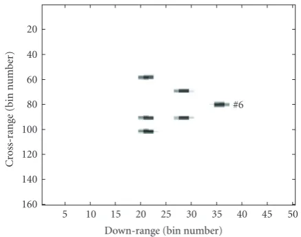
Analytically, the distortion due to phase modulation can be described in terms of a series of higher-order excitation described by the Bessel functions as given in (21). However, it would be more insightful and easier to understand the phase modulation effect by giving a more physical description. Us-ing the temporal motion shown inFigure 9(a)as input, the Doppler frequency for scatterer #1 on the TMS target (see Figure 8(d)) is extracted from the numerical model as a time-frequency spectrogram [9]; this is shown inFigure 12(a). The corresponding distorted ISAR image of scatterer #1 is shown inFigure 12(b). It can be seen that the amount of distortion produced on scatterer #1 in the cross-range is the same as the amount of change in the Doppler frequency (fD,max−fD,min) possessed by scatterer #1 during the imaging interval. This result is expected since the cross-range dimension of the ISAR image is actually the Doppler frequency as explained in Section 3. Note that scatterer #6 in the ISAR image of Figure 12(b)has hardly any distortion. It corresponds to a scatterer located at (x0, 0) inFigure 5. The Doppler frequency of scatterer #6 is shown inFigure 13(a). It is essentially con-stant over the imaging duration; hence there is no noticeable distortion induced in the ISAR image. The phase factor for a small-angle rotation, according to (17), can be approximated by
ψ(t)=exp
−j4π fc c
x0
ω(t)t2
2 −y0ω(t)t
. (23)
50 45 40 35 30 25 20 15 10 5
Down-range (bin number) 160
140 120 100 80 60 40 20
C
ross-r
ange
(bin
n
umber)
(a)
50 45 40 35 30 25 20 15 10 5
Down-range (bin number) 160
140 120 100 80 60 40 20
C
ross-r
ange
(bin
n
umber)
(b)
50 45 40 35 30 25 20 15 10 5
Down-range (bin number) 160
140 120 100 80 60 40 20
C
ross-r
ange
(bin
n
umber)
(c)
5 4 3 2 1 0
−1
−2
−3
−4
Down-range (m)
−4
−3
−2
−1 0 1 2 3 4
C
ross-r
ange
(m)
#1
#2 #3
#4
#5
#6
(d)
Figure8: A sequence of measured ISAR images of the TMS target. (a) constant rotation at 2 degrees/s, (b) oscillating motion introduced to the target’s rotating motion, (c) target with oscillating motion at a later time, and (d) the TMS target’s orientation with respect to the radar for ISAR image in (c). The target is rotated in the counter-clockwise direction.
4 3.5 3 2.5 2 1.5 1 0.5 0
Time (s)
−8
−6
−4
−2 0 2 4
T
arget
ro
tation
ra
te
(deg
re
es/s)
(a)
4 3.5 3 2.5 2 1.5 1 0.5 0
Time (s) 25
26 27 28 29 30 31 32 33 34 35
Re
la
ti
ve
an
gl
e
(d
eg
)
(b)
50 45 40 35 30 25 20 15 10 5
Down-range (bin number) 160
140 120 100 80 60 40 20
C
ross-r
ange
(bin
n
umber)
Figure10: Computed distortion in the ISAR image using the phase modulation model. See and compare with the experimental image inFigure 8(c).
first-order component ω(t)t in (23). It should be stressed that even though the displacementX(t) in a small-angle ro-tation is approximated up to the second order of the Taylor series for the sinusoids of (17), the time-varying rotational rateω(t) in (23) is still given by a sinusoidal function. The sinusoidal function that describesω(t) as given by (14) and (19) can be alternatively expressed using the Taylor series, for example,
sinx=x−x3
3! +
x5 5! −
x7 7! +· · ·
cosx=1−x2
2! +
x4 4! −
x6 6! +· · ·.
(24)
Hence, the time-varying motion of the target described in the present model is consistent with analyses presented in the literature in which the motion is expressed as a Taylor series [3,5]. By expressing the time-varying rotationω(t) using the sinusoidal functions, all the higher-order terms in the Tay-lor series are included implicitly in our model analysis. It is obvious that truncating the Taylor series to the first couple of terms will grossly misrepresent the temporally fluctuat-ing motion and hence the ISAR distortion will not be fully accounted for by the lower-order approximation. The trun-cation of the Taylor series is valid only in the limiting case where the fluctuation in the time-varying motion of the tar-get is not very significant during the imaging period; but this corresponds to a target that has largely a uniform rotational motion, and therefore there is little distortion expected in the ISAR image. We can thus summarize briefly by stating that a changing Doppler frequency of the scatterer due to the target’s time-varying motion expressed through the variable
ω(t) provides the physical basis for the large distortion in the ISAR image.
Another way of seeing the physical interpretation of the phase modulation effect can be illustrated using the exper-imental ISAR image shown in Figure 14(a). This distorted ISAR image provides a convenient illustration since there
exists a down-range bin where there is only one scatterer. The temporal behaviour of the Doppler frequency of this scat-terer extracted using a time-frequency spectrogram is shown inFigure 14(c). Essentially, the spectrogram unfolds the dis-tortion of scatterer #1 in the ISAR image (Figure 14(a)) as a function of time, providing a glimpse of the temporal change in the Doppler frequency during the ISAR imaging duration. In addition, phase information on scatterer #1 is also avail-able from the image data; this is shown inFigure 14(b). It can be clearly seen that the phase is perturbed; that is, not a smooth function in time. By taking the time derivative of the phase, the instantaneous frequency (i.e., 1/2π(dφ/dt) is obtained; this is shown inFigure 14(d). By comparing the Doppler frequency spectrogram inFigure 14(c) and the in-stantaneous frequency inFigure 14(d), it is quite evident that we have arrived at the same temporal history of the Doppler frequency for scatterer #1 via two different directions. From these two graphs, we can make a physical linkage, connecting the distortion introduced in the ISAR image to a time mod-ulation effect in the phase of the scatterer. This illustration provides another perspective on the phase modulation ef-fect. This effect has been validated by experimental data. Ex-amples of the validations are provided by the comparison of the distorted ISAR images betweenFigure 8(c) (experimen-tal) andFigure 10(numerical) and between the experimental image and simulated image inFigure 11. These comparisons have clearly demonstrated that the phase modulation effect offers an accurate picture of the distortion in ISAR images.
6. ISAR DISTORTION ACCORDING TO THE QUADRATIC PHASE EFFECT
It would be helpful and useful to make a comparison of the ISAR distortion as predicted by the phase modulation effect and the quadratic phase effect to see the differences between the two. The quadratic phase distortion assumes a target’s ro-tational motion is constant during the imaging period; that is,ω(t)=ω0. Any change in the Doppler frequency during the imaging duration by any of the scatterers on the target is due to a nonlinear Doppler velocity introduced along the radar’s line of sight as a result of acceleration from the ro-tational motion. This can be seen by substitutingω(t)=ω0 into (23). The phase factor of the rotating scatterer then be-comes
ψ(t)=exp
−j4π fc c
x0
ω0t 2
2 −y0ω0t
. (25)
Considering a scatterer located at (0,y0) on a target as shown inFigure 5, (25) then becomes
ψ(t)=exp
j4π fc c y0ω0t
, (26)
ψ(t) is a linear function in time; therefore, the instantaneous Doppler frequency fD =(2fcy0ω0/c) is a constant. In other words, for scatterers that have motions nearly parallel to the
35 30
25 20
15 10
Down-range (bin number) 3060
3050 3040 3030 3020 3010 3000 2990 2980 2970 2960
C
ross-r
ange
(bin
n
umber)
(a)
35 30
25 20 15
10
Down-range (bin number) 130
120 110 100 90 80 70 60 50 40 30
C
ross-r
ange
(bin
n
umber)
(b)
Figure11: Another example of a comparison between (a) experimental distorted ISAR image and (b) computed distorted ISAR image.
160 140 120 100 80 60 40 20
Time (arb. unit) 30
25 20 15 10 5
Doppler
fr
eq
u
ency
(ar
b
.u
nit)
(a)
50 45 40 35 30 25 20 15 10 5
Down-range (bin number) 160
140 120 100 80 60 40 20
C
ross-r
ange
(bin
n
umber)
#6
#1
(b)
Figure12: (a) Computed Doppler frequency of scatterer #1 on the TMS target during the imaging period, (b) computed ISAR image of scatterer #1 on the TMS target; scatterers #2 and #4 (seeFigure 8(d)) are removed in the computation. The amount of distortion of scatterer #1 corresponds to the amount of change in the Doppler frequency.
located at (x0, 0), (25) becomes
ψ(t)=exp
−j4π fc c x0
ω0t 2
2
. (27)
Equation (27) displays a phase that is a quadratic function in time. Hence, the Doppler frequency will be changing with time, resulting in a blur in the ISAR image.
To see how much a distorting effect the quadratic phase would have on the ISAR image, a constantω0 value corre-sponding to the maximum value of the experimental rota-tional rate, |ωmax| = 3.9 degrees/s (as given by the dashed curve inFigure 9(a)), is used in the numerical model for sim-ulating the TMS target. The resulting ISAR image is shown in Figure 15. The amount of distortion in the image is much less than that for the case where a time-varying rotational rate
ω(t) is used. This is quite evident by comparingFigure 15 withFigure 10.
Another interesting observation that is worthy to note is that in the quadratic phase distortion case, the largest distor-tion occurs at scatterer #6 of the target as seen inFigure 15. The large distortion at scatterer #6 can be explained by the fact that the rate of change of the Doppler frequency is maxi-mum for a scatterer that is moving perpendicular to the radar line of sight (x-axis) as depicted inFigure 5. At the location (x0, 0) and using (12), the movement of scatterer #6 along the
x-axis is given by
x(t)=x0cos
ω0t
. (28)
Its velocity component parallel to the radar line of sight (i.e.,
x-axis) is
vx=dx(t)
dt = −x0ω0sin
ω0t
160 140 120 100 80 60 40 20
Time (arb. unit) 30
25 20 15 10 5
Doppler
fr
eq
u
ency
(ar
b
.u
nit)
(a)
50 45 40 35 30 25 20 15 10 5
Down-range (bin number) 160
140 120 100 80 60 40 20
C
ross-r
ange
(bin
n
umber)
#6
(b)
Figure13: (a) Computed Doppler frequency of scatterer #6 of the TMS target during the imaging period, (b) computed ISAR image of the TMS target with scatterers #2 and #4 removed in the computation. The amount of distortion of scatterer #6 corresponds to the amount of change in the Doppler frequency.
35 30
25 20 15
10
Down-range 3060
3050 3040 3030 3020 3010 3000 2990 2980 2970 2960 2950
C
ross-r
ange
#1
6000 5000 4000 3000 2000 1000 0
Time
Do
p
p
le
r
fr
eq
u
en
cy
a
c
6000 5000 4000 3000 2000 1000 0
Time 0
20 40 60 80 100 120 140
φ
6000 5000 4000 3000 2000 1000 0
Time
−0.05
−0.04
−0.03
−0.02
−0.01 0 0.01 0.02
dφ
/dt
b
d
50 45 40 35 30 25 20 15 10 5
Down-range (bin number) 160
140 120 100 80 60 40 20
C
ross-r
ange
(bin
n
umber)
#6
Figure15: Computed ISAR image of the TMS target using a con-stant rotational rate of 3.9 degrees/s.
to thex-axis; this is intuitively obvious as seen inFigure 5. However, the rate of change ofvxalong the radar line of sight
dvx
dt = −x0ω
2 0cos
ω0t
(30)
is maximum at (x0, 0) because cos(ω0t)= 1 att =0. This implies that the change in the Doppler frequency will be the largest at scatterer #6; therefore, a notable distortion occurs as a result.
To illustrate the distortion’s dependence on (ω0t)2, the ISAR image inFigure 15is generated using a generously large
ω0value; that is,ω0 =3.9 degrees/s. This corresponds to a target rotation of 15.6 degrees over a 4-second imaging time. In the time-varying rotating case (Figure 10), the target rota-tion is only 8.2 degrees over the 4-second durarota-tion. Using a
ω0value corresponding to a target rotation of 8 degrees, the quadratic phase case is computed again using a smallerω0 value of 2 degrees/s. The resulting ISAR image of the target is shown inFigure 16. It can be seen that none of the scat-terers on the target shows any distortion in the image, even scatterer #6 which is expected to display the most distortion. This result is consistent with the experimental ISAR image shown inFigure 8(c), where scatterer #6 displays no notice-able distortion.
As demonstrated in the analysis in this section and in Section 5, it is the temporal variation in the rotation (i.e.,
ω(t)), not the amplitude of the rotation, that introduces the severe distortion in ISAR images. More precisely, the rate of change in the phase of the target echodφ/dt, introduced by the time-varying rotationω(t), produces a band of instan-taneous Doppler frequencies. The distortion in the target’s ISAR image is a result of the introduction of this band of Doppler frequencies during the imaging period. In summary, the above analysis shows that the quadratic phase error is not adequate for describing the severe ISAR distortions that are often seen in the experimental images. The quadratic phase error (i.e., (ω0t)2) is a second-order effect and it produces a
50 45 40 35 30 25 20 15 10 5
Down-range (bin number) 160
140 120 100 80 60 40 20
C
ross-r
ange
(bin
n
umber)
#6
Figure16: Computed ISAR image of the TMS target using a con-stant rotational rate of 2 degrees/s.
much smaller distortion than that from the phase modula-tion effect.
7. REFOCUSING OF DISTORTED ISAR IMAGES
According to the principles of ISAR imaging, a long image integration time is required to produce fine image resolu-tion. However, a long image integration time does not always guarantee good cross-range resolution. This is illustrated in the discussion above where it is found that the amount of blurring from integrating the image over the imaging period can be quite severe. As seen from the discussion above, the blurring of ISAR images is a consequence of a time-varying Doppler frequency due to nonuniform motion of the target during the imaging period. Time-frequency techniques have been used successfully to “refocus” blurred ISAR images. By extracting an ISAR image of the target at a particular instant of time, a better-focused image can be obtained because the target’s motion can be considered as relatively uniform over a short duration. However, there will be a large number of time instants to deal with in time-frequency processing; thus, a large number of refocused ISAR images will be generated, corresponding to different time instants. For accurate target recognition, it is imperative to make use of only the best re-focused image. It is impractical and inefficient to examine all available refocused ISAR images. Visual inspection manually over a large number of images, or even using an automated image search algorithm, only adds extra complexity to the target recognition process.
6000 5000 4000 3000 2000 1000 0
Time (arb. unit)
−4
−3
−2
−1 0 1 2
T
arget
ro
tational
ra
te
(ar
b
.u
nit)
T ta
tb
tc
td
te
tf
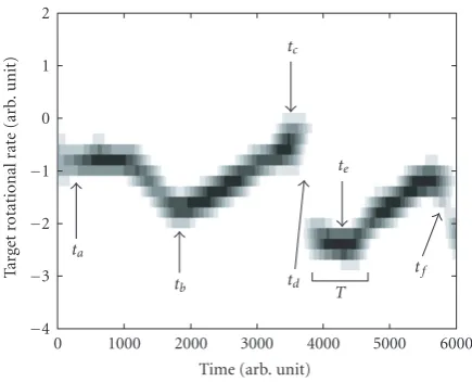
Figure 17: The measured temporal motion of the target corre-sponding to the distorted ISAR image inFigure 11(a).Tis the time window width (0.4 second) used in the refocusing process. Six time instants are chosen for the image refocusing.
distorted image can be refocused efficiently. This image is chosen for its varied time-varying target motion over the imaging period; the corresponding rotational motion of the target is shown inFigure 17.
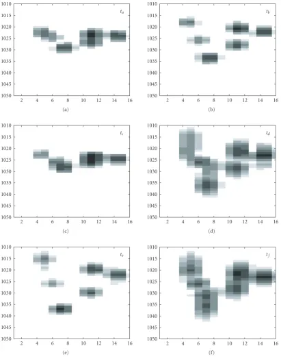
In order to see how an optimum refocused ISAR im-age can be determined, it is helpful to first take a look at some samples of the refocused images at various time in-stants. A refocused ISAR image can be reconstructed from the spectrograms at all the down-range bins of the dis-torted ISAR image at a chosen time instant. The spectro-grams are computed using time-frequency methods [11]. In the example discussed here, spectrograms using short-time Fourier transform (STFT) with a 0.4-second image integra-tion time window is employed. In other words, each refo-cused image is reconstructed from a 0.4-second time seg-ment. Thus it is more accurate to describe a time instant as a short duration of time rather than a precise point in time. Figure 18 shows samples of the refocused ISAR im-ages of the target at the 6 different time instants selected inFigure 17. The ISAR image at timetacorresponds to the instance when the target has a uniform rotational motion. This image serves as a reference image for comparing with the refocused images at other time instants. Using a 0. 4-second STFT, the resolution is just barely adequate to re-solve the scatterers on the target in the cross-range direc-tion for the uniform rotadirec-tion case atta. A quick inspection ofFigure 18reveals that the best refocused images are at the time instantstbandteand the worst images are attc,td, and
tf.
By trying to understand why the worst images are occur-ring attc andtd, and why the best image is located at te, we can develop a methodology for reconstructing the opti-mum refocused ISAR image quickly. The ISAR image attc ap-pears compressed. This is due to a small Doppler frequency (i.e., small angular rotational rate) possessed by the target at this time instant. The Doppler attcis even smaller than the
uniform rotation case at ta; this is illustrated inFigure 17. This Doppler motion is too small to separate the scatterers adequately in the cross-range direction. The ISAR images at timetd andtf still appear blurry, with some of the scatter-ers still not properly focused. This is due to the fact that the Doppler motion of the target is going through a large tempo-ral rate of change within the time windowT; that is, a large (fD,max−fD,min) occurs duringT. In other words, the target is experiencing a range of Doppler frequencies, causing a smear in the image.
The ISAR image atte has all six scatterers on the target clearly resolved and provides the best-refocused image. There are two reasons why the best image quality is found at time instancete. Firstly, the Doppler motion is large, significantly larger than the uniform rotational rate case at the time in-stant ta (see Figure 17). Hence, the scatterers are separated more along the cross-range dimension by the large angular rotational rate of the target. Secondly, the temporal rate of change of the Doppler motion during the time interval atte is small; that is, (fD,max− fD,min)/T is small. Therefore, the blurring of the image is kept to a minimum. The time win-dow widthTat the time instantte is indicated inFigure 17. It can be seen that the rotational motion, hence the Doppler frequency, varies very little within the time window.
Based on the analysis of the refocused images shown in Figure 18, we can deduce a few simple physical rules that will enable us to extract a relatively well-focused image from a blurred ISAR image quickly.
(1) From the blurred image, locate a down-range bin where it contains the most severe blurring in the cross-range. A down-range bin that contains only a single scatterer is desirable, but not necessary.
(2) Produce a time-frequency spectrogram at the chosen down-range bin, using a time-frequency distribution function [11]. Short-time Fourier transform is used here as an illustration. Distribution functions such as the Wigner-Ville distribution and the Choi-Williams distribution may be used; but for targets with multi-ple scatterers, cross-term artifacts from these bilinear distribution functions could be an issue.
(3) From the spectrogram, select a time instant when the variation of the Doppler motion is small (i.e., small (fD,max−fD,min)/T) and the value of the Doppler mo-tion is large (i.e., as far away from the zero Doppler frequency as possible). The time window width T
should be large enough to cover a more or less con-stant Doppler segment.
(4) Construct spectrograms at all down-range bins from the blurred ISAR image of the target. Recombine all spectrograms at the same time instant to reconstruct a focused ISAR image.
16 14 12 10 8 6 4 2 1050 1045 1040 1035 1030 1025 1020 1015 1010
ta
(a)
16 14 12 10 8 6 4 2 1050 1045 1040 1035 1030 1025 1020 1015 1010
tb
(b)
16 14 12 10 8 6 4 2 1050 1045 1040 1035 1030 1025 1020 1015 1010
tc
(c)
16 14 12 10 8 6 4 2 1050 1045 1040 1035 1030 1025 1020 1015 1010
td
(d)
16 14 12 10 8 6 4 2 1050 1045 1040 1035 1030 1025 1020 1015 1010
te
(e)
16 14 12 10 8 6 4 2 1050 1045 1040 1035 1030 1025 1020 1015 1010
tf
(f)
Figure18: Refocused ISAR images of the TMS target from the distorted image inFigure 11(a)at different time instants as indicated in Figure 17.
Although extracting information in a small time inter-val from the original ISAR image data implies a fundamen-tal loss in cross-range resolution, this loss in resolution can be mitigated, however, by a couple of factors. It is interest-ing to note that havinterest-ing a large amount of blurrinterest-ing in the ISAR image may actually be better than having just a small amount of blurring for restoring a focused image. A more se-vere blurring means that at some time instant, there is a large
8. CONCLUSIONS
From the results of the numerical analysis and the compar-isons with experimental data, it is found that the severe dis-tortion in ISAR images can be modelled accurately by in-cluding the temporal variation of the target’s motion in its angular rotational rate. That is to say, the angular rotation is described as a function of time (i.e.,ω(t)) so that an instan-taneous Doppler motion can be ascribed at any given time. A band of instantaneous Doppler frequencies introduced dur-ing the imagdur-ing duration produces a smear in the target’s im-age along the cross-range direction. The distortion mecha-nism can be viewed as a phase modulation effect in the phase of the target echo. The conventional quadratic phase distor-tion is a result of nonlinear Doppler modistor-tion from a target with a constant circular motion and it may be considered as a special case of the phase modulation effect. The quadratic phase error is not adequate to account for the severe distor-tion observed in ISAR images. The phase moduladistor-tion effect is more accurate in quantifying the amount of distortion in ISAR images.
An efficient procedure to find the best-refocused image from a severely blurred image based on time-frequency anal-ysis has also been developed. By applying time-frequency analysis on the distorted target image, one can quickly de-termine the appropriate time instant and the optimum time window width. This information can be used to quickly re-focus the distorted image.
ACKNOWLEDGMENTS
The authors would like to thank V. C. Chen of the Naval Research Laboratory, Washington, for his time and effort in providing comments and inputs to the writing of this manuscript. We would also like to acknowledge the finan-cial support of William Miceli, Office of Naval Research— International Field Office, London, UK, through the NICOP project “Time-Frequency Processing for ISAR Imaging and Non-Cooperative Target Identification” in which the work presented in this manuscript was conducted.
REFERENCES
[1] T. Sparr, S.-E. Hamran, and E. Korsbakken, “Estimation and correction of complex target motion effects ininverse synthetic aperture imaging of aircraft,” inProceedings of IEEE Interna-tional Radar Conference (RADAR ’00), pp. 457–462, Alexan-dria, Va, USA, May 2000.
[2] V. C. Chen and W. J. Miceli, “Simulation of ISAR imaging of moving targets,”IEE Proceedings - Radar, Sonar and Naviga-tion, vol. 148, no. 3, pp. 160–166, 2001.
[3] Y. Wang, H. Ling, and V. C. Chen, “ISAR motion compensa-tion via adaptive joint time-frequency technique,”IEEE Trans-actions on Aerospace and Electronic Systems, vol. 34, no. 2, pp. 670–677, 1998.
[4] D. R. Wehner,High-Resolution Radar, Artech House, Boston, Mass, USA, 2nd edition, 1995.
[5] V. C. Chen and W. J. Miceli, “Time-varying spectral analysis for radar imaging of manoeuvring targets,”IEE Proceedings - Radar, Sonar and Navigation, vol. 145, no. 5, pp. 262–268, 1998.
[6] V. C. Chen and H. Ling,Time-Frequency Transform for Radar Imagery and Signal Analysis, Artech House, Boston, Mass, USA, 2002.
[7] A. W. Rihaczek and S. J. Hershkowitz, “Identification of targets from ISAR images,” inNATO Symposium on Target Identifica-tion and RecogniIdentifica-tion Using RF Systems, Oslo, Norway, October 2004.
[8] T. Sparr and B. Krane, “When are time-frequency methods useful for radar signature analysis,” inNATO Symposium on Target Identification and Recognition Using RF Systems, Oslo, Norway, October 2004.
[9] S. K. Wong, G. Duff, and E. Riseborough, “Distortion in the inverse synthetic aperture radar (ISAR) images of a tar-get with time-varying perturbed motion,”IEE Proceedings -Radar, Sonar and Navigation, vol. 150, no. 4, pp. 221–227, 2003.
[10] S. K. Wong, G. Duff, and E. Riseborough, “Analysis of distor-tion in the high range resoludistor-tion profile from aperturbed tar-get,”IEE Proceedings - Radar, Sonar and Navigation, vol. 148, no. 6, pp. 353–362, 2001.
[11] L. Cohen, “Time-frequency distributions—a review,” Proceed-ings of the IEEE, vol. 77, no. 7, pp. 941–980, 1989.
[12] F. Auger, P. Flandrin, P. Goncalves, and O. Lemoine, “Time-Frequency Toolbox for Use in MATLAB,” Tutorial, July 15, 1997,http://www.nongnu.org/tftb/.
[13] S. K. Wong, E. Riseborough, and G. Duff, “Application of phase modulation to ISAR image processing and counter-measures against radar imaging,” inCombat Identification Sys-tems Conference, Portsmouth, Va, USA, May 2005, Session 5, Paper 6.
S. K. Wong received his B.S. degree in
physics from the University of British Columbia, Canada, in 1978, his M.A.S. and Ph.D. degrees in aerospace science from the University of Toronto in 1980 and 1985, re-spectively. He joined the Defence Research Establishment Valcartier, Canada, in 1986. From 1986 to 1995, he worked on solid-state lasers and nonlinear optics. He moved to the Defence Research Establishment
Ot-tawa in 1995 where he worked on noncooperative target recog-nition, synthetic radar target signature generation, and inverse synthetic aperture radar imaging. Currently, he is working on multistatic SAR/ISAR imaging.
E. Riseboroughreceived the B.Eng. degree
in electrical engineering from Carleton Uni-versity, Ottawa. In 1981, he joined IP Sharp Associates where he worked as a Systems Engineer. In 1987, he joined AIT Corpora-tion where he worked on the development of an experimental array radar system for studying the tracking of low-elevation tar-gets in the presence of multipath. He joined the Defence Research Establishment Ottawa
G. Duffattended the University of Alberta in Electrical Engineering in 1954 and grad-uated from the Southern Alberta Institute of Technology in 1957. He has been em-ployed as a technologist with several Cana-dian government research agencies since the early fifties starting with the Department of Agriculture and subsequently the Defense Research Board, the Communications Re-search Center, the Defense ReRe-search