Volume 2006, Article ID 84797, Pages1–15 DOI 10.1155/ASP/2006/84797
Efficient Fast Stereo Acoustic Echo Cancellation Based on
Pairwise Optimal Weight Realization Technique
Masahiro Yukawa, Noriaki Murakoshi, and Isao Yamada
Department of Communications and Integrated Systems, Graduate School of Science and Engineering, Tokyo Institute of Technology, 2-12-1 Ookayama, Meguro-Ku, Tokyo 152-8550, Japan
Received 1 February 2005; Revised 1 October 2005; Accepted 4 October 2005
In stereophonic acoustic echo cancellation (SAEC) problem, fast and accurate tracking of echo path is strongly required for stable echo cancellation. In this paper, we propose a class of efficient fast SAEC schemes with linear computational complexity (with re-spect to filter length). The proposed schemes are based on pairwise optimal weight realization (POWER) technique, thus realizing a “best” strategy (in the sense of pairwise and worst-case optimization) to use multiple-state information obtained by preprocess-ing. Numerical examples demonstrate that the proposed schemes significantly improve the convergence behavior compared with conventional methods in terms of system mismatch as well as echo return loss enhancement (ERLE).
Copyright © 2006 Masahiro Yukawa et al. This is an open access article distributed under the Creative Commons Attribution License, which permits unrestricted use, distribution, and reproduction in any medium, provided the original work is properly cited.
1. INTRODUCTION
The ultimate goal of this paper is to develop an efficient adap-tive filtering scheme, with linear computational complex-ity, to stably cancel acoustic coupling, from loudspeakers to microphones, occurring in telecommunications with stereo-phonic audio systems. This acoustic coupling is commonly calledacoustic echo(we just call it echo in the following). The stereophonic acoustic echo cancellation (SAEC) problem has become a central issue when we design high-quality, hands-free, and full-duplex systems (e.g., advanced teleconferenc-ing, etc.) [1–13]. A direct application of a monaural echo cancelling algorithm to SAEC usually results in unaccept-ably slow convergence [1–3], and this phenomenon is math-ematically clarified in [5], showing that the normal equation to be solved for minimization of residual echo is often ill-conditioned or has infinitely many solutions due to inherent dependency caused by highly cross-correlated stereo input signals (seeSection 2.2).
Decorrelation of the inputs is a pathway to fast and ac-curate tracking of echo paths (impulse responses), which is necessary for stable echo cancellation [6,8,14,15]. A great deal of effort has been devoted to devise preprocessing of the inputs [3,5,14–22] (see Appendix A). In other words, these preprocessing techniques relax the ill-conditioned situ-ation with use ofadditional informationprovided artificially by feeding less cross-correlated input signals. Based on the
preprocessing [5], real-time SAEC systems have been eff ec-tively implemented, for example, in [8,13]. Under rapidly time-varying situations, however, further convergence ac-celeration is strongly required. Unfortunately, an increase of decorrelation effects by preprocessing may cause audible acoustic distortion or loss of stereo sound effects, thus the preprocessing is strictly restricted to only slight modification of the input signal. The remaining major challenges in SAEC with preprocessing are twofold: (i) fast tracking of the echo paths within the above restriction on audio effects and (ii) low computational complexity due to necessity to adapt 4 echo cancelers with a few thousand taps [7] (seeFigure 1). Now, the time is ripe to move from the early stage of devising preprocessing techniques to the next stage: utilize the addi-tional information provided by preprocessing to the fullest extent possible.
h∗(1)
h∗(2)
Rec.
room nk
u(1)k Unit 1 u(1)
k
h(1)k h(2)k u(2)k
ek(h)
dk − −
+ +
θ(1)
θ(2) sk Talker
Trans. room
Figure1: Stereophonic acoustic echo cancelling scheme; unit 1 is a preprocessing unit (seeAppendix A). Note that the system is not limited to this special structure but can be any appropriate structure.
is reported that it achieves faster convergence in system mis-match,1at the expense of slower convergence in echo return loss enhancement (ERLE), than other major preprocessing techniques such as in [5]. The scheme2proposed in [23] uti-lizes the information from the two states of inputs simulta-neously at each iteration. The two states can be associated with two states of solution sets (mathematically linear vari-eties [5]), sayVandV. By using the adaptive parallel subgra-dient projection (PSP) algorithm [28] (seeSection 3.1), the scheme fairly reduces thezigzag loss3shown inFigure 2(b), and the direction of its update is governed by certain weight-ing factors (seeFigure 2(c)). However, the update direction realized by the uniform weights does not sufficiently approx-imate ideal one. Recently, an efficient strategic weight design called thepairwise optimal weight realization (POWER)was developed in [31,32] for the adaptive PSP algorithm. The POWER technique realizes a best strategy (in the sense of pairwise and worst-case optimization) for the use of multiple information to determine the update direction. This suggests that further drastic acceleration is highly expected by exploit-ing POWER (seeFigure 3).
In this paper, we propose a class of efficient fast SAEC schemes that further accelerate the method in [23] by em-ploying POWER with keeping linear computational com-plexity. In fact, the POWER technique exerts far-reaching effects in a general adaptive filtering application, especially
1Recall that the fast and accurate estimation ofh∗is necessary in SAEC, hence system mismatch is a very important criterion.
2The scheme is derived fromthe adaptive projected subgradient method
[24,25], a unified framework for various adaptive filtering algorithms, which has also been applied to the multiple-access interference suppres-sion problem in DS/CDMA systems successfully [26,27].
3The loss is caused by the “small” angle betweenVandVdue to the
re-striction of “slight” modification in preprocessing (see, e.g., [29, page 197] for angle between subspaces or linear varieties). Similarzigzagbehavior can be observed for alternating projection methods known asKaczmarz’s methodor, more generally, the projections onto convex sets (POCS) in
convex feasibility problem; find a point in the nonempty intersection of
fixedclosed convex sets (see, e.g., [30] andSection 3.1). In the case of two subspacesM1andM2, the rate of convergence of alternating projection
methods is exactly given as (cos(M1,M2))2n−1[29, Theorem 9.31], where
cos(·,·) denotes the cosine of the angle between two subspaces andnthe iteration number. This provides theoretical verification to slow conver-gence caused by the zigzag loss when the angle between two subspaces is small.
h∗
hk ˘
h
V
To identifyh∗
accurately
h∗
V hk
V
To reduce zigzag loss
h∗
V hk
V
(a) Straightforward (b) Conventional (c) UW-PSP
Figure 2: A geometric interpretation of existing methods: (a) straightforward: straightforward application of monaural scheme, (b) conventional: preprocessing-based approach with just one state of inputs at each iteration, (c) UW (uniform weight)-PSP: preprocessing-based approach with two state information at each iteration [23]. The solution setVis periodically changed intoV by preprocessing (VandV arelinear varieties). Note that each arrow of “conventional” stands for the update accumulated during a half-cycle period in which the state of inputs is constant.
when the input signals are highly correlated. Hence, as seen fromFigure 2, POWER is particularly suitable for the SAEC problem. The POWER technique is based on a simple for-mula to give the projection onto the intersection of two closed half-spaces4 that are defined by three vectors (see
Proposition 1). We propose two schemes in the proposed class. The first scheme (Type I) exploits the formula in a combinatorial manner (seeFigure 4(a)). The second scheme (Type II), on the other hand, exploits the formula just once after taking respective uniform averages of projections corre-sponding to each state of inputs (seeFigure 4(b)). The lat-ter scheme is computationally more efficient than the for-mer one, while overall complexities, including the weight de-sign, of both schemes are kept linear with respect to the filter length (seeRemark 1(a)).
4Givenv∈H(H: real Hilbert space) and a closed subspaceM⊂H, the
translation ofMbyvdefines thelinear varietyV:=v+M:= {v+m:m∈ M}. IfM⊥:= {x∈H:x,m =0,∀m∈M}satisfies dim(M⊥)=1,V
is calledhyperplane, which can be expressed asV= {x∈H:a,x =c}
for some (0 =)a∈Handc∈R.Π−:= {x∈H:a,x ≤c}is called a
h∗
hk
V V
Find a best direction by POWER technique
Fast convergence
Figure3: The direction of this paper.
Numerical examples demonstrate that notable improve-ments are achieved, in system mismatch as well as in ERLE, by the use of POWER in place of the uniform weights. Other possible ways to reduce the zigzag loss would be to employ the affine projection algorithm (APA) [33,34] or the recur-sive least-squares (RLS) algorithm [35,36] (the essential dif-ference between our approach and APA is clearly described in
Section 3.2). The proposed schemes are also compared with such other schemes, all of which employ the same prepro-cessing technique as the proposed schemes do. From our nu-merical experiments, we verify superiority of the proposed method. Moreover, we confirm that the proposed schemes exhibit excellent tracking behavior after a change of the echo paths.
2. PRELIMINARIES
2.1. Stereo acoustic echo cancellation problem
Throughout the paper, the following notations are used. Let
L∈N∗:=N\{0}denote the length (of the impulse response)
of the transmission path andN∈N∗the length of the echo
path. For simplicity, let the length of the adaptive filter beN
(analyses for more general cases are presented in [5]). Refer-ring toFigure 1, the signals at timek ∈Nare expressed as follows (the superscriptTstands for transposition):
(i) speech vector:sk∈RL;
(ii)ith transmission path:θ(i)∈RL(i=1, 2); (iii)ith input:u(ki):=sTkθ(i)∈R;
(iv)ith input vector:u(ki):=[u(ki),u (i) k−1,. . .,u
(i)
k−N+1]T ∈RN; (v) preprocessed version ofu(1)k :u(1)k ∈RN;
(vi) input vector:uk:=[u
(1)
k u(2)k
]∈H :=R2N;
(vii) input matrix: Uk := [uk,uk−1,. . .,uk−r+1] ∈ R2N×r (r∈N∗);
(viii) ith echo path:h∗(i)∈RN (i=1, 2); (ix) estimandum:h∗:=[h∗(1)
h∗(2)]∈H;
(x) adaptive filter (echo canceler):hk:=[h
(1)
k h(2)k
]∈H;
(xi) noise:nk:=[nk,nk−1,. . .,nk−r+1]T∈Rr; (xii) output:dk:=UTkh∗+nk∈Rr;
(xiii) residual error function:ek(h) :=UT
kh−dk∈Rr.
Current state 0th stage 1st stage 2nd stage Final stage Previous
state (U1,d1) h
(0)
k,1 h(1)k,(1,5)
(U5,d5) h(0)k,5
(U2,d2) h (0)
k,2 h(0)k,6
(U6,d6)
h(1)k,(2,6) h(2)k,((1,5),(3,7))
(U3,d3)
(U7,d7)
h(0)k,3
h(0)k,7
(U4,d4)
(U8,d8)
h(0)k,4
h(0)k,8
hk+1
h(1)k,(3,7)
h(1)k,(4,8)
h(2)k,((2,6),(4,8))
Projection POWER
(a)
Current state 1st stage 2nd stage (U1,d1)
(U2,d2)
(U3,d3)
(U4,d4)
Previous state (U5,d5)
(U6,d6)
(U7,d7)
(U8,d8)
h(c)k
hk+1
h(p)k
Projection Uniform average POWER
(b)
Figure4: Simple system models with eight parallel processors (q=
4) to implement (a) POWER I and (b) POWER II. For notational simplicity, define the current control sequenceI(c)k = {1, 2, 3, 4}and the previous control sequenceIk(p)= {5, 6, 7, 8}. This type of design of control sequences for POWER I is called binary-tree-like con-struction. It is seen that POWER II is more efficient in computation than POWER I.
The goal of the SAEC problem is to cancel the echostably, that is,uTkh∗−uTkhk≈0, for allk∈N. Since onlyukanddk are observable, a common alternative goal is to suppress the residual echo; that is,ek(hk)≈0, for allk∈N.
2.2. Nonuniqueness problem
In 1991, Sondhi and Morgan found unacceptably slow con-vergence phenomena in SAEC [2] and, in 1995, Sondhi et al. showed that the primitive solution set, obtained from the normal equation to be solved for minimization of the resid-ual echo, is too large and it depends on the transmission paths (due to inherent dependency caused by highly cross-correlated stereo input signals) [3]. This fundamental diffi -culty, deeply seated in SAEC, is commonly referred to as the
nonuniqueness problem, which has earned recognition as an intrinsic burden not existing in the monaural echo cancel-lation. In 1998, Benesty et al. further clarified this problem, and showed that the normal equation is often ill-conditioned or has infinitely many solutions [5].
Let us simply explain the nonuniqueness problem mathe-matically. The input sequence (u(ki))k∈N,i=1, 2, can be
writ-ten as
u(ki)=sk∗θ(i), (1)
where∗denotesconvolution. Considering the case ofN=L, for simplicity,
˘
h:=
˘
h(1) ˘
h(2)
:=h∗+α
θ(2) −θ(1)
, α∈R, (2)
satisfies
i=1,2
u(ki)∗h˘(i)=
i=1,2
u(ki)∗h∗(i), (3)
which implies, under noiseless environments, thatek( ˘h)=0. This is the basic mechanism of the nonuniqueness problem [5] (precise analysis is possible by usingz-transform of (3) with (1); see, e.g., [10]). From (2), we see that filter coeffi -cients that cancel the echo depend on the transmission paths θ(1)andθ(2). This implies that, without well-approximating
h∗, echo will relapse by change ofθ(1)andθ(2)due to talker’s alternation, and so forth (see also [23, Appendix A]). Hence, it is strongly desired to keephkclose toh∗before the trans-mission paths change drastically.
3. PROPOSED CLASS OF STEREO ACOUSTIC ECHO CANCELLATION SCHEMES
In this section, we present a class of set-theoretic SAEC schemes based on the POWER weighting technique. The proposed approach utilizes parallel projection onto certain closed convex sets. First, we provide a brief introduction of set-theoretic adaptive filtering and define the closed convex sets. Then, we show the relationship between the proposed approach and the APA-based method. Finally, we present the proposed schemes in a simple manner.
3.1. Set-theoretic adaptive filtering and convex set design
We briefly introduce the basic idea of theset-theoretic [24,
25,28, 37, 38]/set-membership[39, 40] approaches in the adaptive filtering. Let us first start with the set-theoretic ap-proach5 in the static convex feasibility problem[30,37,38,
41]; find a point in the nonempty intersection offixedclosed convex setsSi,i∈ I⊂N. Each setSiis designed based on available information, such as noise statistics and observed data, so thatSicontains the estimandumh∗with high prob-ability. Suppose thath∗ ∈Si, for alli∈I. Then, it is a nat-ural strategy to find a point ini∈ISias an estimate ofh∗. Due to the nonlinear nature of the problem, certain succes-sive numerical approximations by utilizing the information on each setSiinfinitely many times are, in general, necessary. In [28], the adaptive filtering problem is translated into a
time-varyingversion of the convex feasibility problem, where multiple closed convex sets S(ik),i ∈ Ik ⊂ N, are defined by multiple observable data, hence being time-varying (a unified framework for this approach is found in [24,25]). Namely, the collection of convex sets (S(ik))i∈Ik used at time kis varying based on data incoming from one minute to the next (alsoh∗is possibly time-varying). Especially in rapidly time-varying environments, it should be reasonable to use a limited number of sets (S(ik))i∈Ik that are defined with re-cently obtained data. This strategy agrees with saving the computational complexity, another requirement in adaptive filtering. This is the basic idea of the set-theoretic adaptive filtering approach.
The adaptive PSP algorithm [28] was proposed as an ef-ficient set-theoretic adaptive filtering technique. The algo-rithm adoptssubgradient projectionsas approximations of the exact projections onto the convex sets for saving the compu-tation costs. The multiple (subgradient) projections are com-puted in parallel, hence the algorithm can save, by engaging parallel processors, the time consumption for each update. Finally, the update direction of filter is determined by taking a weighted average of the projections.
The first step is to define closed convex sets that contain
h∗with high probability. A possible choice is as follows [28]:
Cι(ρ) :=h∈H:=R2N :gι(h) :=eι(h)2
−ρ≤0, ∀ι∈Ik⊂N, ∀k∈N, (4)
whereρ ≥ 0 andIk is the control sequence at timek(see
Section 3.3). Assignment of an appropriate value toρraises the membership probability Prob{h∗ ∈ Cι(ρ)}and, at the same time, keeps Cι(ρ) sufficiently small (see Section 3.2
for detailed discussion). Since the projection ontoCι(ρ) re-quires, in general, very high computational complexity, we
5 The difference is clearly stated in [37] between the set-theoretic approach
instead employ the projection onto the closed half-space6 [28]Hι−(hk) := {x∈H :x−hk,∇gι(hk)+gι(hk)≤0} ⊃
Cι(ρ), which has the following simple closed-form expres-sion:
PHι−(hk)(h)
=
⎧ ⎪ ⎪ ⎪ ⎨ ⎪ ⎪ ⎪ ⎩
h+−gι
hk +
hk−h T
∇gι
hk
∇gι
hk 2
∇gι
hk ifh ∈Hι−
hk ,
h otherwise.
(5)
Here,∇gι(hk) = 2Uιeι(hk) andPHι−(hk)(h) ∼= PCι(ρ)(h); see
[28, Figure 3]. It should be remarked thatPHι−(hk)(h) requires O(N) complexity. Choosing speciallyh=hk, we have
PHι−(hk)(hk)
=
⎧ ⎪ ⎪ ⎨ ⎪ ⎪ ⎩
hk− gι
hk
∇gι
hk 2 ∇gι
hk ifhk ∈Hι−
hk ,
hk otherwise.
(6)
3.2. Relationship to APA-based method and robustness issue against noise
The popular APA [34] can be viewed in the time-varying set-theoretic framework [28] with the linear varietiesVk := arg minh∈Hek(h)2 (∀k ∈ N). The APA generates a
se-quence of filtering vectors (hk)k∈N ⊂ H(:= R2N) by (see
[28])
hk+1=hk+λk
PVk
hk −hk , ∀k∈N, (7)
whereλk∈(0, 2). In particular, forr =1, (7) is nothing but the normalized least-mean-square (NLMS) algorithm [43], whereris the dimension of affine projection (seeSection 2.1
for the definitions ofUk ∈R2N×r anddk ∈ Rr). A simple comparison ofVkwithCk(ρ) in (4) implies thatVk=Ck(δk), whereδk:=minh∈Hek(h)2. Note here that we most likely haveδk≈0, since we often have 2Nrdue to long impulse responses of acoustic paths.
The remains of this section is devoted to therobustness issue against noise by highlighting the membership h∗ ∈
Ck(ρ), which ensures the monotone approximation property (for stability), that is,hk+1−h∗ ≤ hk−h∗. Noting that
h∗∈Ck(ρ)⇔ ek(h∗)2= n
k2≤ρ, we see thatρgoverns the reliability on the membershiph∗ ∈Ck(ρ) by0ρfr(ξ)dξ, where fr(ξ) is the probability density function (pdf) of the random variableξ:= nk2, (fr(ξ) is given in [28, Equation (9)]). Under the assumption that the noise process is a zero-mean i.i.d. Gaussian random variableN(0,σ2), the random variableξfollows aχ2distribution (of orderr), whereσ2is
6Tighter closed half-spaces are also presented in [42], which can also be
used with the proposed schemes.
the variance of noise. The pdf fr(ξ) is strictly monotone de-creasing overξ ≥0 forr =1, 2, whereas forr ≥3, it has its unique peak atξ=(r−2)σ2and fr(0)=limξ
→∞fr(ξ)=0.
Recall that we most likely haveδk ≈0. The above facts im-ply that forr ≥ 3, Prob{h∗ ∈ Ck(δk)(= Vk)}is expected to be small, which causes serious sensitivity of the APA to noise forr ≥ 3 (seeSection 4). Forr = 1, 2, on the other hand, Prob{h∗ ∈Ck(δk)}is expected to be relatively large, which suggests robustness of the APA (r =1, 2) against noise (this agrees with theH∞optimality [44] of the NLMS, a spe-cial case of the APA forr = 1). By designing appropriateρ
based on statistics of noise process (see [28, Example 1]), the proposed schemes can fairly raise Prob{h∗ ∈ Ck(ρ)}; note that Prob{h∗∈Hk−(hk)} ≥Prob{h∗∈Ck(ρ)}because
Hk−(hk)⊃ Ck(ρ). This brings about the noise robustness of POWER I/II inSection 3.3.
3.3. Novel POWER-based stereo echo canceler
Givenq∈N∗, define thecontrol sequenceconsisting of theq
latest time indices asIk(c):= {k,k−1,. . .,k−q+ 1} ⊂N. Let
Q ∈ N∗ denote the cycle period of preprocessing [14,15],
that is, everyQ/2 iterations, the state of inputs is switched. Then,k−Q/2 (∀k > Q/2) always belongs to the state op-posite tok. To utilize data from both states of inputs, we use
I(c) k ∪I
(p)
k as in [23], where
I(p) k :=
⎧ ⎪ ⎪ ⎨ ⎪ ⎪ ⎩
∅, 0≤k≤Q 2,
I(c)
k−Q/2, k >
Q
2.
(8)
Note that the definitions ofI(c)k andI(p)k can be generalized to any index sets consisting of arbitrary indices chosen from the current and previous states, respectively (see [45]). For simplicity, however, we focus on the above specific definition in the following.
The most important definition is now given: three-point expression of projection onto the intersection of two closed half-spaces. For convenience, let us define that for alla,b∈
H,
Π−(a,b) :=y∈H:a−b,y−b ≤0⊂H, (9)
where Π−(a,b) is a closed half-space ifa = b. Then, for a given ordered triplet (s,a,b) ∈ H3such that Π−(s,a)∩
Π−(s,b) = ∅, we define
P(s,a,b) :=PΠ−(s,a)∩Π−(s,b)(s), (10)
We propose a new class of SAEC schemes that utilizeP(s,
a,b) (Proposition 1) to realize better weights in the method proposed in [23] (seeAppendix B). Two schemes in the pro-posed class are presented below, where two families of closed half-spaces, {Hι−(hk)}ι∈I(c)
k and{H
−
ι (hk)}ι∈I(p)
k , are used in different ways.
3.3.1. POWER Type I
A scheme that exploits the POWER technique in a combi-natorial manner is presented below (seeFigure 4(a)). Define
I(1)
k := {(k−i+ 1,k−Q/2−i+ 1) : i = 1, 2,. . .,q} ⊂ {(ι1,ι2) : ι1 ∈ I(c)k , ι2 ∈ Ik(p)}. Also define inductively the control sequences used in each stage as I(km) ⊂ {(ι1,ι2) :
ι1,ι2 ∈Ik(m−1), ι1 =ι2},∀m∈ {2, 3,. . .,M}, for allk ∈N, satisfying 1= |I(M)
k ||I (M−1)
k | ≤ · · · ≤ |I (2) k | ≤ |I
(1) k | =q. The scheme is given as follows.
Scheme 1 (POWER Type I). Suppose that a sequence of closed convex sets (Ck(ρ))k∈N ⊂H is defined as in (4). Let h0∈Hbe an arbitrarily chosen initial vector. Then, define a sequence of filtering vectors (hk)k∈N⊂H through multiple
stages.
0th stage: projection onto2qhalf-spaces
hk(0),ι :=PHι−(hk)hk , ∀k∈N,∀ι∈I(c)k ∪Ik(p), (11)
wherePH−ι(hk)(hk) is computed by (6).
1st∼Mth stage: find good direction
form:=1toMdo
h(km,ι):=
⎧ ⎪ ⎪ ⎨ ⎪ ⎪ ⎩
hk ifη(km,ι)= −
ξk(m,ι)ζk(m,ι) =0,
Phk,h(km,ι1−1),h(km,ι2−1) otherwise,
∀k∈N, ∀ι=ι1,ι2 ∈I(km), (12)
whereη(km,ι) := h (m−1) k,ι1 −hk,h
(m−1)
k,ι2 −hk,ξ (m) k,ι := h
(m−1) k,ι1 −
hk2, andζk(m,ι):= h (m−1) k,ι2 −hk
2.
end.
Final stage: update to good direction
hk+1:=hk+λk
h(kM,ι)−hk
, ∀k∈N, (13)
whereλk∈[0, 2] is the step size.
Through the multiple stages, the direction of update is improved thanks to the operatorP(·,·,·) (see [32] for de-tails).
3.3.2. POWER Type II
A simple and efficient scheme that exploits the POWER tech-nique just once is given as follows (seeFigure 4(b)).
Scheme 2 (POWER Type II). Suppose that a sequence of closed convex sets (Cι(ρ))ι∈I⊂His defined as in (4), where I := k∈N(I(c)k ∪I
(p)
k ). Leth0 ∈H be an arbitrarily cho-sen initial vector. Then, define a sequence of filtering vectors (hk)k∈N⊂Hthrough the following two stages.
1st stage: uniformly averaged directions
h(g)k
:=
⎧ ⎪ ⎪ ⎪ ⎪ ⎨ ⎪ ⎪ ⎪ ⎪ ⎩
hk+M(g)k
⎛ ⎜ ⎝
ι∈I(g)
k
wk(g)PHι−(hk)
hk −hk
⎞ ⎟
⎠ ifI(g)k = ∅,
hk otherwise,
∀k∈N, ∀g∈ {c, p}, (14)
wherew(g)k :=1/|I(g)
k | =1/q(∀ι∈I (g) k ) and
M(g) k
:=
⎧ ⎪ ⎪ ⎪ ⎪ ⎨ ⎪ ⎪ ⎪ ⎪ ⎩
ι∈I(g)
k w
(g)
k PHι−(hk)hk−hk2
ι∈I(g)
k w
(g)
k PHι−(hk)hk −hk
2 ifhk ∈
ι∈I(g)
k H
−
ι
hk ,
1 otherwise.
(15)
2nd stage: reasonably averaged direction by POWER
hk+1:=
⎧ ⎪ ⎨ ⎪ ⎩
hk ifηk=−
ξkζk =0,
hk+λk
Phk,h(c)k ,h(p)k −hk
otherwise, (16)
for allk∈N, whereλk∈[0, 2] is the step size,ηk := h(c)k −
hk,h(p)k −hk,ξk:= h(c)k −hk2, andζk:= h(p)k −hk2.
In the 1st stage, for saving the computational complex-ity, the uniform averagesh(c)k andh(p)k are computed for two groups corresponding toI(c)k andIk(p). In the 2nd stage, the POWER technique is exploited to find a good direction of update based on three kinds of information:hk,h(c)k , andh(p)k
Hk−−Q/2(hk) Π−(h
k,h(p)k ) Hk−−Q/2−1(hk)
h(1)k,(k,k−Q/2) hII
k+1 h(c)k
V(θ1)
h∗
hk
Hk−(hk) Π−(h
k,h(c)k ) Hk−−1(hk)
hIk+1
h(1)k,(k−1,k−Q/2−1)
h(p)k
V(θ1)
Figure 5: A geometric interpretation of the proposed schemes. POWER I:hI
k+1, POWER II:hIIk+1. The control sequences are defined
asI(c)k = {k,k−1}andI
(p)
k = {k−Q/2,k−Q/2−1}. The dotted area showsι∈I(c)
k ∪I
(p)
k H
− ι (hk).
Remark 1. (a) Simple system models to implement the pro-posed schemes with q = 4 are shown in Figure 4. The structure of POWER I is namedbinary-tree-like construction
with its number of stages M = log2q+ 1; in this case,
M = 3 (see [31,32]). We see that POWER II is more ef-ficient in computational complexity than POWER I, since it utilizes the POWER technique just once. The projections {PHι−(hk)(hk)}
ι∈I(c)
k ∪I
(p)
k , for all k ∈ N, in (11) and (14) are, respectively, computed simultaneously with 2q concurrent processors. This implies that the proposed schemes are in-herently suitable for implementation with concurrent pro-cessors. With such processors, the number of multiplications imposed on each processor is (3M+ 2r + 1)N + 21M+r
(M = log2q+ 1) for POWER I and (2r + 6)N +r for POWER II forq≥2; forq=1, it is reduced to (2r+ 4)N+r
for POWER I/II (see [32]). In other words, the complexity is keptO(N), which is a desired property especially for real-time implementation.
(b) Discussions about convergence of the adaptive PSP algorithm are found in the adaptive projected subgradient method [24, 25], a more general framework. A geometric interpretation illustrated in Figure 5 will be rather help-ful from a standpoint of application. For simplicity, we set q = 2 and λk = 1. In the figure, the estimandum
h∗ (see Section 2.1) is assumed to belong to the dotted area, that is, h∗ ∈ ι∈I(c)
k∪I
(p)
k H
−
ι (hk). This assumption holds ifCk(ρ) is defined appropriately (for details, see [28]). We see that the schemes realize good directions of update. For visual clarity, the half-spaces Π−(hk,hk(1),(k,k−Q/2)) and
Π−(h
k,h(1)k,(k−1,k−Q/2−1)) are omitted. It is not hard to see that
hk+1 = P(hk,hk(1),(k,k−Q/2),h (1)
k,(k−1,k−Q/2−1)) = h (1)
k,(k,k−Q/2) in this simple example.
(c) The proposed schemes realize strategic weight designs for the method in [23] in the sense that the schemes give op-timal weights, based on a certain max-min criterion, in each stage, see AppendicesCandD.
0.8 0.4 0
−0.4
−0.8
A
m
plitude
0 1 2 3 4 5
Samples (×105) u(1)k
(a) 0.8
0.4 0
−0.4
−0.8
A
m
plitude
0 1 2 3 4 5
Samples (×105) u(2)k
(b)
Figure6: The input signals (u(1)k )k∈Nand (u(2)k )k∈N. The signals are
generated from a speech signal, sampled at 8 kHz, of an English na-tive male.
4. NUMERICAL EXAMPLES
This section presents numerical examples of the proposed schemes, the UW-PSP [23] (seeAppendix B), APA [33,34], NLMS [43], and fast RLS (FRLS) [36, 46] algorithms. All the methods are performed with a common preprocessing technique in [14,15] that periodically delays input signals in the 1st channel with the cycle of preprocessing Q = 2000. The tests are conducted, for estimatingh∗ ∈ H :=
R2000(N =L=1000), under the noise situation of SNR := 10 log10(E{z2
k}/E{n2k}) = 25 dB, wherezk := uk,h∗ and
E{·}denotepure echo(i.e., echo without noise) and expec-tation, respectively. We utilize a recorded speech signal of an English native male7 shown inFigure 6, for (sk)k
∈N, which
was sampled at 8 kHz. For numerical stability against the poorly excited inputs observed inFigure 6, all the algorithms are regularized. The APA is regularized by following the way in [47] with exactly the same parameter as in [28]. The NLMS is regularized by following the way in [35, Equation (9.144)] with the regularization parameter δ = 1.0×10⁻¹ for better performance. Because the original RLS algorithm is computationally intensive for acoustic echo cancellation applications [11, page 77], a simplified implementation of the regularized RLS [46] is employed withξk2 = 20σu2 and
φk=1 (∀k∈N), whereσu2is the variance of (uk)k∈N. For the
proposed schemes and the UW-PSP, the projection in (6) is
7The speech sample is provided by “Special Research Project of the
0
−10
−20
−30
Sy
st
em
mismat
ch
(dB)
0 1 2 3 4 5
Iteration number (×105)
NLMS
Proposed-I (q=4)
UW-PSP (q=16)
Proposed-I (q=16) Proposed-II (q=16)
Proposed-I (q=4)
(a)
25 20 15
10 5 0
ERLE
(dB)
0 1 2 3 4 5
Iteration number (×105)
NLMS
Proposed-I (q=4)
UW-PSP (q=16)
Proposed-II (q=16) Proposed-I (q=16)
(b)
Figure7: Proposed schemes versus UW-PSP forr=1 andλk=0.4 under SNR=25 dB. For a comparison, the performance of NLMS (a special case of the proposed method forq=1) is shown forλk=0.2.
regularized as
PH(δι−)(hk)(hk)
:=
⎧ ⎪ ⎪ ⎨ ⎪ ⎪ ⎩
hk− gι
hk
∇gι
hk 2+δ ∇gι
hk ifhk ∈Hι−
hk ,
hk otherwise,
(17)
whereδ is set to 1.0×10⁻⁶. In addition to the regulariza-tion for numerical stability against poor excitaregulariza-tion, while the signal power is less than a common threshold, we stop the update for all algorithms throughout the simulations (this is the reason of the observable flat intervals in the figures).
To measure the achievement level for echo-path identifi-cation as well as echo cancellation, the following criteria are evaluated:
system mismatch (k) :=10 log10h
∗−h
k2
h∗2 , ∀k∈N,
ERLE (k) :=10 log10
k i=1zi2
k i=1
zi−
ui,hi 2
, ∀k∈N.
(18)
Simulations are conducted under several conditions.
4.1. Proposed schemes versus UW-PSP with differentq
First, we examine the performance of the proposed schemes and the UW-PSP with (|I(c)
k | = |I (p)
k | =)q=4, 16 inFigure 7. For a comparison, the curve of NLMS with the step sizeλk= 0.2 is drawn, which is a special case of POWER I for q = 1,r =1,ρ=0,λk=0.4,Ik(0)=I
(c)
k = {k},I (1)
k = {(k,k)} (M=1), and I(p)k = ∅. For the proposed schemes, we set
λk=0.4 (∀k ∈N),r =1, andρ=max{(r −2)σ2, 0} =0, seeSection 3.2and [28]. The control sequences for POWER I are designed in the same manner as shown inFigure 4.
For POWER II and the UW-PSP, the curves ofq = 4 are omitted for visual clarity, since the difference between
q = 4 andq = 16 is not significant. Referring toFigure 7, we see that the increase ofqfor POWER I significantly im-proves the convergence speed without serious degradation in steady-state performance in both criteria. We also see that POWER I forq=4 exhibits faster convergence than the UW-PSP forq =16. The above observation suggests thatweight design is the key to attain better performance by increasingq.
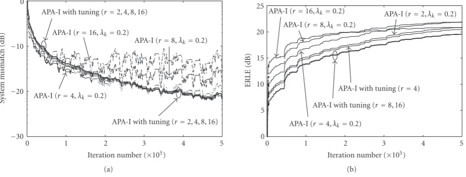
4.2. APA-based method with differentr
Next, we examine the performance of the APA for r = 2, 4, 8, 16 inFigure 8, whereris the dimension of affine pro-jection (seeSection 3.2). The APA-based method using data from one state of inputs at each iteration is referred to as “APA-I.” The step size forr =2 is set toλk =0.2 for better performance. Forr = 4, 8, 16, two step sizes are employed; one is fixed toλk =0.2 (the same step size asr =2), for all
r, and the other is individually tuned, for eachr, so that the steady-state performance in system mismatch is almost the same asr=2 withλk=0.2.
Referring to Figure 8, the increase of r for the APA-I raises the initial convergence speed at the expense of seri-ous degradation in the steady-state performance in system mismatch, which causes gain loss in ERLE especially forr = 8, 16. For the tuned step size, on the other hand, no distinct difference is observed among allrin system mismatch, since, for larger, the small step size for good steady-state perfor-mance decreases the initial convergence speed. Comparing
Figure 8withFigure 7, it is seen that POWER I successfully alleviates the tradeoffproblem between convergence speed and steady-state performance.
0
−10
−20
−30
Sy
st
em
mismat
ch
(dB)
0 1 2 3 4 5
Iteration number (×105)
APA-I (r=4,λk=0.2)
APA-I with tuning (r=2, 4, 8, 16) APA-I (r=8,λk=0.2) APA-I (r=16,λk=0.2)
APA-I with tuning (r=2, 4, 8, 16)
(a)
25 20 15 10 5 0
ERLE
(dB)
0 1 2 3 4 5
Iteration number (×105)
APA-I (r=4,λk=0.2)
APA-I with tuning (r=8, 16) APA-I with tuning (r=4)
APA-I (r=16,λk=0.2) APA-I (r=2,λk=0.2) APA-I (r=8,λk=0.2)
(b)
Figure8: APA-I forr=2, 4, 8, 16 under SNR=25 dB. Forr=2, we setλk=0.2. Forr=4, 8, 16, we use the same step sizeλk =0.2 and individually tuned one;λk=0.1 forr=4,λk=0.04 forr=8, andλk=0.022 forr=16.
0
−10
−20
−30
Sy
st
em
mismat
ch
(dB)
0 1 2 3 4 5
Iteration number (×105)
FRLS
NLMS
APA-I
UW-PSP (q=8) Proposed-II (q=8) Proposed-I (q=8)
(a)
25 20 15 10 5 0
ERLE
(dB)
0 1 2 3 4 5
Iteration number (×105)
Proposed-I (q=8) Proposed-II (q=8)
UW-PSP (q=8)
APA-I
NLMS
FRLS (fair ERLE)
FRLS
(b)
Figure9: Proposed schemes versus UW-PSP, NLMS, and APA-I under SNR=25 dB. For the NLMS,λk =0.2. For the APA-I,r =2 and λk=0.15. For the FRLS,γ=1−1/18N. For the proposed schemes and the UW-PSP,r=1,λk=0.4, andq=8.
colored excited input signals, without severely deteriorating the steady-state performance (see, e.g., [48–51]). Under low-SNR situations, on the other hand, it is theoretically verified that the increase ofr in the APA decreases the membership probabilityh∗ ∈Vk(especially forr ≥3, Prob(h∗ ∈Vk)≈ 0) [28, Section III], which causes serious noise sensitivity of the APA forr≥3 (see alsoSection 3.2).
4.3. Proposed schemes versus UW-PSP, APA, NLMS, and FRLS with fixed and time-varying echo paths
The proposed schemes are now compared with the UW-PSP, APA-I, NLMS, and FRLS algorithms in Figures9and10. For the proposed schemes and the UW-PSP, the parameters are exactly the same as inFigure 7except thatq = 8. For the
NLMS, the step size is set to 0.2 to attain better steady-state performance. For the APA-I, we setr =2 andλk =0.15 so that the initial convergence speed is the same as the UW-PSP. For the FRLS, the forgetting factor is set toγ=1−1/18Nfor the best performance among our experiments. We remark that the FRLS algorithm exhibits severe sensitivity against the choice of the forgetting factor or the regularization parame-terξ2
k; for example, once we tried to employγ=1−1/15N, the speed of convergence was a little faster but the filter di-verged around the iteration number 500000. In this simula-tion, although the steady-state performance is not the same as the proposed schemes, the parameters are tuned care-fully.
0
−10
−20
−30
Sy
st
em
mismat
ch
(dB)
0 1 2 3 4 5
Iteration number (×105)
FRLS NLMS
APA-I
FRLS
NLMS
APA-I
Proposed-I (q=8) Proposed-II (q=8)
UW-PSP (q=8)
(a)
25 20 15 10
5 0
ERLE
(dB)
0 1 2 3 4 5
Iteration number (×105)
Proposed-I (q=8) Proposed-II (q=8)
UW-PSP (q=8)
APA-I
NLMS FRLS (fair ERLE)
FRLS
FRLS (fair ERLE) NLMS & APA
(b)
Figure10: Proposed schemes versus UW-PSP, NLMS, and APA-I with the echo paths changed at the iteration number 1.6×10⁵. The other
conditions are the same as inFigure 9.
Table 1: Time needed to achieve the system mismatch level of
−20 dB.
Method POWER I POWER II UW-PSP FRLS APA-I NLMS
Second 25 31 43 28 50 75
much faster convergence as well as better steady-state per-formance than the NLMS, APA-I, and FRLS algorithms. The time for POWER I to achieve the system mismatch level of −20 dB is approximately 25 second. The time for each algo-rithms is summarized inTable 1. POWER I is approximately 45 second, 25 second, and 3 second faster than the NLMS, the APA-I, and the FRLS, respectively.Figure 10depicts the re-sults under the condition where the echo-paths are changed at the iteration number 1.6×10⁵. We see that the proposed schemes exhibit excellent tracking behavior against echo path variation. In Figures9and10, the FRLS exhibits poor ERLE performance due to the observable instability in system mis-match at the beginning of adaptation. For fairness, we also draw the curves of the FRLS in a different ERLE criterion in which the summations are taken (not from i = 1 but) from the moment when its system mismatch becomes less than 0 dB (this new ERLE criterion is referred to as “fair ERLE”).
It is reported that the RLS algorithm exhibits, besides its high computational complexity, an instability issue especially for (nonstationary) speech signals, and thus has been dis-couraged to be used in acoustic echo cancellation [11, page 77]. Also the FRLS algorithms inherit the instability issue, as pointed out in a considerable amount of literature, for exam-ple, [7, page 40], [52–55]. Moreover, the observable slow ini-tial convergence of the FRLS stems from the same reason as its tracking inferiority, under nonstationary environments, to the LMS-type algorithms, as remarked, for example, in [44,56,57].
4.4. Proposed schemes versus APA with simultaneous use of data from two states
Finally, POWER I is compared, in Figure 11, with the re-maining possibility to resolve thezigzag loss(seeSection 1), that is, the APA with simultaneous use of data from two states of inputs. Namely, for allk≥Q/2 +r/2,ek(h) :=UT
kh−dk is used to defineVk(seeSection 3.2) instead ofek(h), where
Uk :=[uk· · ·uk−r/2+1uk−Q/2· · ·uk−Q/2−r/2+1]∈R2N×r and
dk := UTkh∗+nk ∈Rr withnk :=[nk,. . .,nk−r/2+1,nk−Q/2,
. . .,nk−Q/2−r/2+1]T. This new APA method is referred to as “APA-II.” For the proposed scheme, the parameters are the same as inFigure 7(or inFigure 9) forq=4, 8. For the APA-II, for fairness,r = 8, 16 are employed with the tuned step sizes λk = 0.04, 0.022, respectively. For a comparison, the curves of APA-I and II withr = 2 and λk = 0.2 are also drawn.
In Figure 11, we observe that the proposed scheme achieves faster initial convergence and better steady-state performance than the APA-II in both criteria. Moreover, for the APA-II, the increase ofrimproves the initial convergence speed at the expense of unignorable deterioration in ERLE. On the other hand, for the proposed scheme, the increase of
qimproves the performance in both criteria, as also shown inFigure 7.
5. CONCLUSION
0
−10
−20
−30
Sy
st
em
mismat
ch
(dB)
0 1 2 3 4 5
Iteration number (×105)
APA-II (r=2) APA-II (r=8)
APA-II (r=16)
APA-I (r=2)
Proposed-I (q=8) Proposed-I (q=4)
Proposed-I (q=8)
(a)
25 20 15 10 5 0
ERLE
(dB)
0 1 2 3 4 5
Iteration number (×105)
Proposed-I (q=8) Proposed-I (q=4)
APA-I & II (r=2) APA-II (r=8, 16)
(b)
Figure11: Proposed schemes (q=4, 8) versus APA-II (r=2, 8, 16) under SNR=25 dB. For the proposed schemes, we employ the same parameters as inFigure 7. For APA-II,λk=0.2, 0.04, 0.022 forr=2, 8, 16, respectively. For APA-I,r=2 andλk=0.2.
APPENDICES
A. PREPROCESSING TECHNIQUES
As stated inSection 2.2, the difficulty of nonuniqueness has been known to be inherent in the SAEC problem. To al-leviate this difficulty, several excellent preprocessing tech-niques8were proposed; half-wave rectifier [5] (see [22] for an improved version), comb filtering [3,17], additive noise [18,19], and time-varying filtering [14–16], (see [21] for a generalized version of [14]); another nonlinear preprocess-ing technique is also proposed in [20]. Indeed, efficacy of sev-eral nonlinear preprocessing techniques was quantified with mutual coherence of the stereo inputs [62].
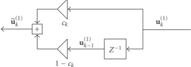
Figure 12illustrates a simple example of the preprocess-ing unit generatpreprocess-ing two states of inputs (see alsoFigure 1). In [14,15], it is reported that periodic one-sample delays, in one side of stereo inputs (i.e.,u(1)k inFigure 1), realize accu-rate echo-path identification without audible degradation in speech. Sinceu(1)k is generated by convolution of the talker’s speechsk with the transmission path θ(1), the periodic de-lays virtually give one-sample shift toθ(1). In other words, the preprocessing technique introduces a slightly modified state of input and alternates two9(modified and nonmod-ified) states of inputs periodically, leading to alternation of two states of transmission path, sayθ(1)andθ(1). As a result, since the solution set depends on transmission paths as men-tioned above, two slightly different solution sets,V(θ(1)) and
V(θ(1)) (corresponding toV andV inFigure 2, resp.), are generated alternately.
8Some nonpreprocessing techniques were also proposed with an advantage
of no degradation in input signals [58–61], however, their tracking speed of echo paths is somewhat inferior to some preprocessing techniques.
9Although the number of states could be generalized to more than two by
generating more than one modified state, we adopt two states for simplic-ity.
u(1)k
+ ck
1−ck
u(1)k−1
u(1)k
Z−1
Figure12: A preprocessing unit called input sliding. The factorck slides between 0 and 1 periodically, and thus,u(1)k :=cku(1)k + (1− ck)u(1)k−1is a periodically delayed version ofu
(1)
k .
B. SAEC SCHEME PROPOSED IN [23]
Scheme 3(see [23]). Suppose that a sequence of closed con-vex sets (Cι(ρ))ι∈I ⊂ H is defined as in (4), whereI :=
k∈N(I(c)k ∪I (p)
k ). Let h0 ∈ H be an arbitrarily chosen initial vector. Then, define a sequence of filtering vectors (hk)k∈N⊂Hby
hk+1:=hk+λkMk
⎛ ⎜ ⎝
ι∈I(c)
k∪I
(p)
k
w(ιk)PH−ι(hk)hk −hk
⎞ ⎟ ⎠,
(B.1) for allk∈N, whereλk∈[0, 2] is the step size, (w(ιk))ι∈I(c)
k ∪I
(p)
k , for allk ∈ N, are the weights satisfyingwι(k) ∈ [0, 1], and
ι∈I(c)
k∪I
(p)
k w
(k)
ι =1, and
Mk:=
⎧ ⎪ ⎪ ⎪ ⎪ ⎪ ⎪ ⎪ ⎪ ⎨ ⎪ ⎪ ⎪ ⎪ ⎪ ⎪ ⎪ ⎪ ⎩
ι∈I(c)
k∪I
(p)
k w
(k)
ι PHι−(hk)hk −hk2
ι∈I(c)
k∪I
(p)
k w
(k)
ι PHι−(hk)hk −hk
2
ifhk ∈
ι∈I(c)
k∪I
(p)
k H
−
ι
hk ,
1 otherwise.
(B.2)
Ifwι(k) = 1/2q(∀ι ∈ I(c)k ∪I (p)
C. COMPUTATION OFP(s,a,b)AND PAIRWISE-OPTIMALITY
The following proposition gives an efficient way to calculate
P(s,a,b) with given (s,a,b)∈H3.
Proposition 1 (projection onto intersection of two half-spaces [32]). Given(s,a,b)∈H3s.t.Π−(s,a)∩Π−(s,b) =
∅, letξ := a−s2,ζ := b−s2, andη:= a−s,b−s.
Then,
P(s,a,b)=s+μ∗ω∗a+1−ω∗ b−s, (C.1)
where
μ∗:=
⎧ ⎪ ⎪ ⎪ ⎨ ⎪ ⎪ ⎪ ⎩
1 ifη≥ξorη≥ζ,
2ξζ−(ξ+ζ)η
ξζ−η2 ifη <min{ξ,ζ},
ω∗:=
⎧ ⎪ ⎪ ⎪ ⎪ ⎪ ⎪ ⎪ ⎨ ⎪ ⎪ ⎪ ⎪ ⎪ ⎪ ⎪ ⎩
1 ifη≥ζ,
0 ifζ > η≥ξ,
ζ(ξ−η)
2ξζ−(ξ+ζ)η ifη <min{ξ,ζ}.
(C.2)
Let us define the operatorQ: [0, 1]×[0,∞)×H3→H by
Q(ω,μ,s,a,b) :=s+μωa+ (1−ω)b−s. (C.3)
By (C.1) and (C.3), we see thatP(s,a,b) = Q(ω∗,μ∗,s,
a,b). An optimality ofω∗andμ∗is shown below.
Proposition 2 (optimality of ω∗ and μ∗ [32]). Given (s,
a,b) ∈ H3 s.t. Π−(s,a)∩Π−(s,b) = ∅, let φ(ω,μ,z) :=
s−z2−Q(ω,μ,s,a,b)−z2. Then,(ω∗,μ∗)inProposition 1is optimal in the sense of
ω∗,μ∗ ∈ arg max (ω,μ)∈[0,1]×[0,∞)
min z∈Π−(s,a)∩Π−(s,b)
φ(ω,μ,z). (C.4)
Intuitively, (ω∗,μ∗) achieves a worst-case optimization, or, in other words, (C.4) implies that (ω∗,μ∗) is a solution to the max-minproblem of maximizing, overωandμ, the minimum ofφ(ω,μ,z) overz. A geometric interpretation of Propositions1and2is given inFigure 13.
Another proposition is presented below to show an opti-mality of the weights realized by the proposed schemes.
Proposition 3(see [32]). Supposeh∗ ∈ ι∈I(c)
k∪I
(p)
k H
−
ι (hk),
k∈N. Then, the following hold:
(I)h∗∈Π−(hk,h(m)
k,ι ),∀ι∈I (m)
k ,∀m∈ {1,. . .,M−1}, (II)h∗∈Π−(hk,h(c)
k )∩Π−(hk,h (p) k ).
For POWER I, Propositions2and3(I) imply that the di-rection of update is getting improved step by step through multiple stages, since the weights realized in each stage are
Π−(s,a)∩Π−(s,b) z
P(s,a,b)
Q(ω,μ,s,a,b) 1−ω∗
a ω
∗
b
Π−(s,a)
1−ω s
ω Π
−(s,b)
Figure13: A geometric interpretation of Propositions1and2. Let
hk := sand hk+1 := Q(ω,μ,s,a,b). Then,s−z = hk−z and Q(ω,μ,s,a,b)−z = hk+1 −zdenote the distance to z[∈ Π−(s,a)∩Π−(s,b)] from the filtering vector before and af-ter update, respectively.Proposition 2means that (ω∗,μ∗) given in
Proposition 1maximizes minz∈Π−(s,a)∩Π−(s,b)hk−z2−hk+1−z2.
optimalin the sense of a solution to a worst-case optimiza-tion problem. For POWER II, similarly, Proposioptimiza-tions2and
3(II) imply that the weights realized in the second stage are
optimal.
D. WEIGHT REALIZATION
In this appendix, we show that POWER I and POWER II can be written in the form of the scheme proposed in [23], which is given inAppendix B. The weights realized by POWER I are given as follows.
Proposition 4(weight realization by POWER I [32]). Let
(hk)k∈N ⊂H be a sequence of filtering vectors generated by Scheme 1. Then,hk+1 is represented in the form ofScheme 3
with(w(jk)=w (k) j,ι,M)j∈I(c)
k∪I
(p)
k , for allk∈N, satisfying thatw
(k) j >0
andj∈I(c)
k∪I
(p)
k w
(k)
j =1, wherew (k)
j,ι,Mis defined by the following
simple recursive form: ifη(km,ι)= −
ξk(m,ι)ζ (m)
k,ι =0, thenw (k) j,ι,m=0 (∀m=1, 2,. . .,M,∀ι∈I(m)
k ,∀j∈I (c) k ∪I
(p)
k ), otherwise,
w(jk,ι),1:=
⎧ ⎪ ⎪ ⎪ ⎪ ⎪ ⎨ ⎪ ⎪ ⎪ ⎪ ⎪ ⎩
ω∗ ifι=(j,·),
1−ω∗ ifι=(·,j),
0 otherwise,
∀j∈I(c) k ∪I
(p)
k , ∀ι∈I (1) k ,
w(jk,ι),m:=
ω∗μ∗Lw (k) j,ιL,m−1+
1−ω∗ μ∗Rw (k) j,ιR,m−1 ω∗μ∗
L+
1−ω∗ μ∗
R
,
∀j∈I(c) k ∪I
(p) k , ∀ι=