Dereverberation by Using Time-Variant Nature of Speech Production System

Volume 2007, Article ID 65698,15pages doi:10.1155/2007/65698

Research Article

Dereverberation by Using Time-Variant Nature of

Speech Production System

Takuya Yoshioka, Takafumi Hikichi, and Masato Miyoshi

NTT Communication Science Laboratories, NTT Corporation 2-4, Hikaridai, Seika-cho, Soraku-gun, Kyoto 619-0237, Japan Received 25 August 2006; Revised 7 February 2007; Accepted 21 June 2007

Recommended by Hugo Van hamme

This paper addresses the problem of blind speech dereverberation by inverse filtering of a room acoustic system. Since a speech signal can be modeled as being generated by a speech production system driven by an innovations process, a reverberant signal is the output of a composite system consisting of the speech production and room acoustic systems. Therefore, we need to extract only the part corresponding to the room acoustic system (or its inverse filter) from the composite system (or its inverse filter). The time-variant nature of the speech production system can be exploited for this purpose. In order to realize the time-variance-based inverse filter estimation, we introduce a joint estimation of the inverse filters of both the time-invariant room acoustic and the time-variant speech production systems, and present two estimation algorithms with distinct properties.

Copyright © 2007 Takuya Yoshioka et al. This is an open access article distributed under the Creative Commons Attribution License, which permits unrestricted use, distribution, and reproduction in any medium, provided the original work is properly cited.

1. INTRODUCTION

Room reverberation degrades speech intelligibility or cor-rupts the characteristics inherent in speech. Hence, deberation, which recovers a clean speech signal from its rever-berant version, is indispensable for a variety of speech pro-cessing applications. In many practical situations, only the reverberant speech signal is accessible. Therefore, the dere-verberation must be accomplished with blind processing.

Let an unknown signal transmission channel from a source to possibly multiple microphones in a room be mod-eled by a linear time invariant system (to provide a unified description independent of the number of microphones, we refer to a set of signal transmission channel(s) from a source to possibly multiple microphones as a signal transmission channel. The channel from the source to each of the micro-phones is called a subchannel. A set of signal(s) observed by the microphone(s) is refered to as an observed signal. We also refer to an inverse filter set, which is composed of fil-ters applied to the signal observed by each microphone, as an inverse filter). The observed signal (reverberant signal) is then the output of the system driven by the source signal (clean speech signal). On the other hand, the source signal is modeled as being generated by a time variant autoregressive (AR) system corresponding to an articulatory filter driven by an innovations process [1]. In what follows, for the sake of

definiteness, the AR system corresponding to the articula-tory filter and the system corresponding to the room’s signal transmission channel are refered to as thespeech production systemand theroom acoustic system, respectively. Then, the observed signal is also the output of the composite system of the speech production and room acoustic systems driven by the innovations process. In order to estimate the source signal, the dereverberation may require the inverse filter of the room acoustic system. Therefore, blind speech derever-beration involves the estimation of the inverse filter of the room acoustic system separately from that of the speech pro-duction system under the condition that neither the param-eters of the speech production system nor those of the room acoustic system are available.

Several approaches to this problem have already been in-vestigated. One major approach is to exploit the diversity be-tween multiple subchannels of the room acoustic system [2–

6]. This approach seems to be sensitive to order misdetec-tion or additive noise since it strongly exploits the isomor-phic relation between the subspace formed by the source sig-nal and that formed by the observed sigsig-nal. The so-called prewhitening technique achieved some positive results [7–

this technique regards the residual signal generated by ap-plying LP to the observed signal as the output of the room acoustic system driven by the innovations process. Then, the inverse filter of the room acoustic system can be obtained by using methods designed for i.i.d. series. Although methods incorporating this technique may be less sensitive to addi-tive noise than the subspace approach, the dereverberation performance remains insufficient since the heuristics is just a crude approximation. Also methods that estimate the source signal directly from the observed signal by exploiting features inherent in speech such as harmonicity [11] or sparseness [12] have been proposed. The source estimate is then used as a reference signal when calculating the inverse filter of the room acoustic system. However, the influence of source es-timation errors on the inverse filter estimates remains to be revealed, and a detailed investigation should be undertaken.

As an alternative to the above approach, the time variant nature of the speech production system may help us to ob-tain the inverse filter of the room acoustic system separately from that of the speech production system. Let us consider the inverse filter of a composite system consisting of speech production and room acoustic systems. The overall inverse filter is composed of the inverse filters of the room acoustic and speech production systems. The inverse filter of the room acoustic system is time invariant while that of the speech pro-duction system is time variant. Hence, if it is possible to ex-tract only the time invariant subfilter from the overall inverse filter, we can obtain the inverse filter of the room acoustic sys-tem. This time-variance-based approach was first proposed by Spencer and Rayner [13] in the context of the restora-tion of gramophone recordings. They implemented this ap-proach simply; the overall inverse filter is first estimated, and then, it is decomposed into time invariant and time variant subfilters. However, it would be extremely difficult to obtain an accurate estimate of the overall inverse filter, which has both time invariant and time variant zeros especially when the sum of the orders of both systems is large [14]. There-fore, the method proposed in [13] is inapplicable to a room environment.

This paper proposes estimating both the time invariant and time variant subfilters of the overall inverse filter directly from the observed signal. The proposed approach skips the estimation of the overall inverse filter, which is the drawback of the conventional method. Let us consider filtering the ob-served signal with a time invariant filter and then with a time variant filter. When the output signal is equalized with the innovations process, the time invariant filter becomes the in-verse filter of the room acoustic system whereas the time vari-ant filter negates the speech production system. Thus, we can obtain the inverse filter of the room acoustic system simply by adjusting the parameters of the time invariant and time variant filters so that the output signal is equalized with the innovations process. We then propose two blind processing algorithms based on this idea. One uses a criterion involving the second-order statistics (SOS) of the output; the other uti-lizes the higher-order statistics (HOS). Since SOS estimation demands a relatively small sample size, the SOS-based algo-rithm will be efficient in terms of the length of the observed signals. On the other hand, the HOS-based algorithm will

provide highly accurate inverse filter estimates because the HOS brings additional information. Performance compar-isons revealed that the SOS-based algorithm improved the rapid speech transmission index (RASTI), which is a measure of speech intelligibility, from 0.77 to 0.87 by using observed signals of at most five seconds. In contrast, the HOS-based al-gorithm estimated the inverse filters with a RASTI of nearly one when observed signals of longer than 20 seconds were available. The main variables used in this paper are listed in

Table 1as a reference.

2. PROBLEM STATEMENT

2.1. Problem formulation

The problem of speech dereverberation is formulated as fol-lows. Let a source signal (clean speech signal) be represented bys(n), and the impulse response of anM×1 linear finite im-pulse response (FIR) system (room acoustic system) of order

K by{h(k)=[h1(k),. . .,hM(k)]T}0≤k≤K. SuperscriptT in-dicates the transposition of a vector or a matrix. An observed signal (reverberant signal)x(n)=[x1(n),. . .,xM(n)]Tcan be modeled as

x(n)= K

k=0

h(k)s(n−k). (1)

Here,x(n) consists ofMsignals from theMmicrophones. By using the transfer function of the room acoustic system, we can rewrite (1) as

x(n)=H(z)s(n), (2)

H(z)= K

k=0

h(k)z−k_=H

1(z),. . .,HM(z)

T

, (3)

where [z−1] represents a backward shift operator.Hm(z) is the transfer function of the subchannel ofH(z), correspond-ing to the signal transmission channel from the source to the mth microphone. Then, the task of dereverberation is to recover the source signal from N samples of the ob-served signal. This is achieved by filtering the obob-served sig-nalx(n) with the inverse filter of the room acoustic system H(z). Lety(n) denote the recovered signal and let{g(k) = [g1(k),. . .,gM(k)]T}−∞≤k≤∞ be the impulse response of the inverse filter. Then,y(n) is represented as

y(n)=

∞

k=∞

g(k)T_{x(n−k), (4)}

or equivalently,

y(n)=G(z)Tx(n), (5)

G(z)=

∞

k=∞

g(k)z−k. (6)

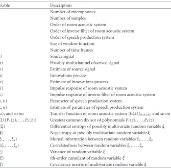
Table1: List of main variables.

Variable Description

M Number of microphones

N Number of samples

K Order of room acoustic system

L Order of inverse filter of room acoustic system P Order of speech production system

W Size of window function

T Number of time frames

s(n) Source signal

x(n) Possibly multichannel observed signal y(n) Estimate of source signal

e(n) Innovations process

d(n) Estimate of innovations process

h(k) Impulse response of room acoustic system

g(k) Impulse response of inverse filter of room acoustic system b(k,n) Parameter of speech production system

a(k,n) Estimate of parameter of speech production system

H(z), and so on Transfer function of room acoustic system{h(k)}0≤k≤K, and so on GCD{P1(z),. . .,Pn(z)} Greatest common divisor of polynomialsP1(z),. . .,Pn(z)

H(ξ) Differential entropy of possibly multivariate random variableξ J(ξ) Negentropy of possibly multivariate random variableξ I(ξ1,. . .,ξn) Mutual information between random variablesξ1,. . .,ξn K(ξ1,. . .,ξn) Correlatedness between random variablesξ1,. . .,ξn υ(ξ) Variance of random variableξ

κi(ξ) ith-order cumulant of random variableξ

Σ(ξ) Covariance matrix of multivariate random variableξ

equalized with the source signals(n) up to a constant scale and delay. This requirement can also be stated as

G(z)T_H(z)=αz−β_{, (7)}

whereαandβare constants representing the scale and delay ambiguity, respectively.

Next, the model of the source signals(n) is given as fol-lows. A speech signal is widely modeled as being generated by a nonstationary AR process [1]. In other words, the speech signal is the output of a speech production system modeled as a time variant AR system driven by an innovations process. Let{b(k,n)}n∈Z, 1≤k≤P, whereZis the set of integers, denote the time dependent parameters of the speech production sys-tem of orderPand lete(n) denote the innovations process. Then,s(n) is described as

s(n)= P

k=1

b(k,n)s(n−k) +e(n), (8)

or equivalently,

s(n)=

1 1−B(z,n)

e(n), (9)

B(z,n)= P

k=1

b(k,n)z−k_{. (10)}

In this paper, we assume that

(1) the innovations{e(n)}n∈Zconsist of zero-mean

inde-pendent random variables,

(2) the speech production system 1/(1−B(z,n)) has no time invariant pole. This assumption is equivalent to the following equation:

GCD. . ., 1−B(z, 0), 1−B(z, 1),. . .=1, (11) where GCD{P1(z),. . .,Pn(z)} represents the greatest common divisor of polynomialsP1(z),. . .,Pn(z).

Although assumption (1) does not hold for a voiced portion of speech in a strict sense due to the periodic nature of vo-cal cord vibration, the assumption has been widely accepted in many speech processing techniques including the linear predictive coding of a speech signal. A comment on the va-lidity of assumption (2) is provided inSection 4.

2.2. Fundamental problem

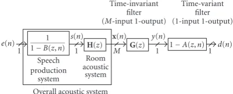
Figure 1depicts the system that produces the observed signal from the innovations process. We can see that the observed signal is the output ofH(z)/(1−B(z,n)), which we call the overall acoustic system, driven by the innovations process.

Overall acoustic system Speech production

system (1-input 1-output)

Room acoustic system (1-inputM-output) e(n)

1 1 M

1 1−B(z,n)

s(n)

H(z) x(n)

Figure1: Schematic diagram of system producing observed signal

from innovations process.

by assumption (1); neither the parameters of 1/(1−B(z,n)) nor those ofH(z) are available. Therefore, we face the criti-cal problem of how to obtain the inverse filter ofH(z) sep-arately from that of 1/(1−B(z,n)) with blind processing. This is the cause of the so-called excessive whitening problem [6], which indicates that applying methods designed for i.i.d. series (e.g., see [15,16] and references therein) to a speech signal results in cancelling not only the characteristics of the room acoustic systemH(z) but also the average characteris-tics of the speech production system 1/(1−B(z,n)).

3. TIME-VARIANCE-BASED APPROACH

In order to overcome the problem mentioned above, we have to exploit a characteristic that differs for the room acous-tic system H(z) and the speech production system 1/(1−

B(z,n)). We use the time variant nature of the speech pro-duction system as such a characteristic.

Let us consider the inverse filter of the overall acoustic systemH(z)/(1−B(z,n)). Since the overall acoustic system consists of a time variant part 1/(1−B(z,n)) and a time in-variant partH(z), the inverse filter accordingly has both time invariant and time variant zeros. The set of time invariant ze-ros forms the inverse filter of the room acoustic systemH(z) while the time variant zeros constitute the inverse filter of the speech production system 1/(1−B(z,n)). Hence, we can obtain the inverse filter of the room acoustic system by ex-tracting the time invariant subfilter from the inverse filter of the overall acoustic system.

3.1. Review of conventional methods

A method of implementing the time-variance-based inverse filter estimation is proposed in [13,17]. The method pro-posed in [13, 17] identifies the speech production system and the room acoustic system assuming that both systems are modeled as AR systems. The overall acoustic system is first estimated from several contiguous disjoint observation frames. In this step, it is assumed that the overall acous-tic system is time invariant within each frame. Then, poles commonly included in the framewise estimates of the over-all acoustic system are collected to extract the time invariant part of the overall acoustic system.

Overall acoustic system Speech

production system

Room acoustic

system

Time-invariant filter (M-input 1-output)

Time-variant filter (1-input 1-output) e(n)

1 1 M 1 1

1 1−B(z,n)

s(n)

H(z)

x(n)

G(z) y(n)

1−A(z,n) d(n)

Figure 2: Schematic diagram of global system from innovations

process to its estimate.

The method imposes the following two conditions.

(i) The frame size is larger than the order of the room acoustic system as well as that of the speech produc-tion system.

(ii) None of the system parameters change within a single frame.

However, the parameters of the speech production system change by tens of milliseconds while the order of the room acoustic system may be equivalent to several hundred mil-liseconds. Therefore, we can never design a frame size that meets those two conditions. This frame-size problem is dis-cussed in more detail inSection 3.2.

Moreover, this method assumes that the room acoustic system is minimum phase, which may be an unrealistic as-sumption. Therefore, it is difficult to apply this method to an actual room environment.

Reference [14] proposes another method of implement-ing the time-variance-based inverse filter estimation. The method estimates only the room acoustic system based on maximum a posteriori estimation assuming that the inno-vations process e(n) is Gaussian white noise. However, the method also assumes the room acoustic system to be mini-mum phase.

3.2. Novel method based on joint estimation of time invariant/time variant subfilters

The two requirements for the frame size with the conven-tional method arise from the fact that it estimates the overall acoustic system in the first step. Therefore, we propose the joint estimation of the time invariant and time variant subfil-ters of the inverse filter of the overall acoustic system directly from the observed signalx(n).

Let us consider filtering x(n) with time invariant fil-ter G(z) and then with time variant filter 1−A(z,n) (see

Figure 2). If we represent the parameters of 1−A(z,n) by {a(k,n)}1≤k≤P, the final outputd(n) is given as follows:

d(n)=y(n)− P

k=1

or equivalently,

d(n)=1−A(z,n)y(n), (13)

A(z,n)= P

k=1

a(k,n)z−k_{, (14)}

wherey(n) is given by (5). Then, we have the following the-orem under assumption (2).

Theorem 1. Assume that the final output signald(n)is equal-ized with innovations processe(n)up to a constant scale and delay, and that1−A(z,n)has no time invariant zero:

d(n)=αe(n−β), (15)

GCD1−A(z, 1),. . ., 1−A(z,N)=1. (16)

Then, the time invariant filterG(z)satisfies(7).

Proof. The proof is given inAppendix A.

This theorem states that we simply have to set up the tap weights{gm(k)}1_{and{a(k,n)}so thatd(n) is equalized with} αe(n−β). The calculated time invariant filter G(z) corre-sponds to the inverse filter of the room acoustic systemH(z), and the time variant filter 1−A(z,n) corresponds to that of the speech production system 1/(1−B(z,n)). Thus, we can conclude that the joint estimation of the time invariant/time variant subfilters is a possible solution to the problem de-scribed inSection 2.2.

At this point, we can clearly explain the drawback of the conventional method with a large frame size. When using a large frame size, it is impossible to completely equalized(n) withαe(n−β) because 1/(1−B(z,n)) varies within a single frame. Hence, the estimate of the overall acoustic system in each frame is inevitably contaminated by estimation errors. These errors make it difficult to extract static poles from the framewise estimates of the overall acoustic system. By con-trast, the joint estimation that we propose does not involve the estimation of the inverse filter of the overall acoustic sys-tem. Therefore, a frame size shorter than the order of the room acoustic system can be employed, which enables us to equalized(n) withαe(n−β).

Since the innovations processe(n) is inaccessible in real-ity, we have to develop criteria defined solely by usingd(n). These criteria are provided in the next two sections. The al-gorithms derived can deal with a nonminimum phase system as the room acoustic system since they use multiple micro-phones and/or the HOS of the outputd(n) [15,16].

4. ALGORITHM USING SECOND-ORDER STATISTICS

Since output signald(n) is an estimate of innovations process

e(n), it would be natural to set up the tap weights{gm(k)} and{a(k,n)}so that the statistical property of the outputs

1_{Hereafter, we will omit the range of indices unless necessary.}

{d(n)}1≤n≤N satisfies assumption (1). In this section, we de-velop a criterion based only on the SOS of{d(n)}. To be more precise, we try to uncorrelate{d(n)}.

We assume the following two conditions additionally in this section.

(i) M≥2, that is, we use multiple microphones.

(ii) Subchannel transfer functionsH1(z),. . .,HM(z) have no common zero.

Under these assumptions, the observed signalx(n) is an AR process driven by the source signals(n) [16]. Therefore, we can substitute an FIR inverse filter of orderLfor the doubly-infinite inverse filter in (4) as

y(n)= L

k=0

g(k)Tx(n−k). (17)

Here, we can restrict the first tap ofG(z) as

gm(0)=

⎧ ⎪ ⎨ ⎪ ⎩

1 m=1,

0 m=2,. . .,M,

(18)

where the microphone withm =1 is nearest to the source (see [16] for details).

4.1. Loss function

LetK(ξ1,. . .,ξn) denote a suitable measure of correlatedness between random variables ξ1,. . .,ξn. Then, the problem is mathematically formulated as

minimize {a(k,n)},{gm(k)}

Kd(1),. . .,d(N)

subject to1−A(z,n)_1≤n≤N being minimum phase. (19)

The constraint of (19) is intended to stabilize the estimate, 1/(1−A(z,n)), of the speech production system.

First, we need to define the correlatedness measureK(·). Several criteria for measuring the correlatedness between random variables have been developed [18,19]. We use the criterion proposed in [19] since it can be further simplified as described later. The criterion is defined as

Kξ1,. . .,ξn

= n

i=1 logυξi

−logdetΣ(ξ), (20)

ξ=ξn,. . .,ξ1

T

, (21)

whereυ(ξ1),. . .,υ(ξn), respectively, represent the variances of random variablesξ1,. . .,ξn, andΣ(ξ) denotes the covariance matrix ofξ. Definition (20) is a suitable measure of correlat-edness in that it satisfies

Kξ1,. . .,ξn

≥0 (22)

with equality if and only if random variables ξ1,. . .,ξnare uncorrelated as

i= j⇐⇒Eξiξj

whereE{·}denotes an expectation operator. Then, we will try to minimize

Kd(1),. . .,d(N)= N

n=1

logυd(n)−logdetΣ(d), (24)

d=d(N),. . .,d(1)T (25)

with respect to{a(k,n)}and{gm(k)}. This loss function can be further simplified as follows under (18) (seeAppendix B):

Kd(1),. . .,d(N)= N

n=1

logυd(n)+ constant. (26)

Hence, problem (19) is finally reduced to

minimize {a(k,n)},{gm(k)}

N

n=1

logυd(n)

subject to1−A(z,n)being minimum phase.

(27)

Therefore, we have to set up tap weights {a(k,n)} and {gm(k)}under (18) so as to minimize the logarithmic mean of the variances of outputs{d(n)}.

Next, we show that the set of 1−A(z,n) andG(z) that minimizes the loss function of (27) equalizes the output sig-nald(n) with the innovations processe(n).

Theorem 2. Suppose that there is an inverse filter, G(z), of the room acoustic system that satisfies (7) and (18). Then,

N

n=1logυ(d(n))achieves a minimum if and only if

d(n)=αe(n−β)=h1(0)e(n). (28)

Proof. The proof is presented inAppendix C.

With Theorems1and2, a solution to problem (27) pro-vides the inverse filters of the room acoustic system and the speech production system.

Remark 1. Let us assume that the variance ofd(n) is station-ary. The loss function of (27) is then equal toNlogυ(d(n)). Because the logarithmic function is increasing monotoni-cally, the loss function is further simplified to Nυ(d(n)), which may be estimated byNn=1d(n)2. Thus, the loss func-tion of (27) is equivalent to the traditional least squares (LS) criterion when the variance ofd(n) is stationary. However, since the variance of the innovations process indeed changes with time, the loss function of (27) may be more appropriate than the LS criterion. This conjecture will be justified by the experiments described later.

4.2. Algorithm

In this section, we derive an algorithm for accomplishing (27). Before we proceed, we introduce an approximation of time variant filter 1−A(z,n). Since a speech signal within a

short time frame of several tens of milliseconds is almost sta-tionary, we approximate 1−A(z,n) by using a filter that is globally time variant but locally time invariant as

1−A(z,n)=1−Ai(z), i=

n−1

W + 1

, (29)

where W is the frame size and · represents the floor function. Under this approximation,d(n) is produced from

y(n) as follows. The outputs{y(n)}1≤n≤N, ofG(z) are seg-mented into T short time frames by using a W-sample rectangular window function. This generates T segments {y(n)}N1≤n≤N1+W−1,. . .,{y(n)}NT≤n≤NT+W−1, whereNiis the

first index of theith frame satisfyingN1=1,NT+W−1=N, andNi+W=Ni+1. Then,y(n) in theith frame is processed through 1−Ai(z) to yieldd(n) as

d(n)=y(n)− P

k=1

ai(k)y(n−k). (30)

By using this approximation, problem (27) is reformulated as

minimize

{ai(k)}1≤i≤T, 1≤k≤P,{gm(k)}1≤m≤M, 1≤k≤L

N

n=1

logυd(n)

subject to1−Ai(z)_1≤i≤Tbeing minimum phase.

(31)

We solve problem (31) by employing an alternating vari-ables method. The method minimizes the loss function with respect first to{ai(k)}for fixed{gm(k)}, then to{gm(k)}for fixed{ai(k)}, and so on. Let us represent the fixed value of

gm(k) bygm(k) and that ofai(k) byai(k). Then, we can for-mulate the optimization problems for estimating{ai(k)}and {gm(k)}as

minimize {ai(k)}1≤i≤T, 1≤k≤P

N

n=1

logυd(n)

{gm(k)}={gm(k)}

subject to1−Ai(z)being minimum phase,

(32)

minimize {gm(k)}1≤m≤M, 1≤k≤L

N

n=1

logυd(n)

{ai(k)}={ai(k)}

. (33)

Note that only{gm(k)}with k ≥ 1 are adjusted. The first tap weights{gm(0)}are fixed as (18). By repeating the opti-mization cycle of (32) and (33)R1times, we obtain the final estimates ofai(k) andgm(k).

First, let us derive the algorithm that accomplishes (32). We first note that (32) is achieved by solving the following problem for each frame numberi:

minimize {ai(k)}1≤k≤P

Ni+W−1

n=Ni

logυd(n)

{gm(k)}={gm(k)}

subject to 1−Ai(z) being minimum phase.

(34)

Let us assume thatd(n) is stationary within a single frame. Then, the loss function of (34) becomes

Ni+W−1

n=Ni

Furthermore, because of the monotonically increasing prop-erty of the logarithmic function, the loss function be-comes equivalent to Nυ(d(n)), which can be estimated by Ni+W−1

n=Ni d(n)

2_{. Thus, the solution to (34) is obtained}

by minimizing the mean square of d(n). Such a solu-tion is calculated by applying linear predicsolu-tion (LP) to {y(n)}Ni≤n≤Ni+W−1. It should be noted that LP guarantees

that 1−Ai(z) is minimum phase when the autocorrelation method is used [1].

Next, we derive the algorithm to solve (33). We realize (33) by using the gradient method. By calculating the deriva-tive of loss functionN_n=1logυ(d(n)), we obtain the follow-ing algorithm (seeAppendix Dfor the derivation):

gm(k)=gm(k) +δ

T

i=1

d(n)vm,i(n−k)

Ni+W−1

n=Ni

d(n)2Ni+W−1

n=Ni

, (36)

vm,i(n)=xm(n)− P

k=1

ai(k)xm(n−k), (37)

where·Ni+W−1

n=Ni is an operator that takes an average from Nith to (Ni+W−1)th samples, andδis the step size. The up-date procedure (36) is repeatedR2times. Since the gradient-based optimization of{gm(k)}is involved in each (32)-(33) optimization cycle, (36) is performedR1R2times in total.

Remark 2. Now, let us consider the special case ofR1 = 1. Assume that we initialize{gm(k)}as

gm(k)=0, 1≤ ∀m≤M, 1≤ ∀k≤L. (38)

Then,{ai(k)}is estimated via LP directly from the observed signal, and{gm(k)}is estimated by using those estimates of {ai(k)}. This is essentially equivalent to methods that use the prewhitening technique [7–10]. In this way, the prewhiten-ing technique, which has been used heuristically, is derived from the models of source and room acoustics explained in

Section 2. Moreover, by repeating the (32)-(33) cycle, we may obtain more precise estimates.

4.3. Experimental results

We conducted experiments to demonstrate the performance of the algorithm described above. We took Japanese sen-tences uttered by 10 speakers from the ASJ-JNAS database [20]. For each speaker, we made signals of various lengths by concatenating his or her utterances. These signals were used as the source signals, and by using these signals, we could investigate the dependence of the performance on the sig-nal length. The observed sigsig-nals were simulated by convolv-ing the source signals with impulse responses measured in a room. The room layout is illustrated inFigure 3. The or-der of the impulse responses,K, was 8000. The reverberation time was around 0.5 seconds. The signals were all sampled at 8 kHz and quantized with 16-bit resolution.

The parameter settings are listed inTable 2. The initial estimates of the tap weights were set as

gm(k)=0, 1≤ ∀m≤M, 1≤ ∀k≤L (39)

while{gm(0)}1≤m≤Mare fixed as (18).

Room: 200 cm height Source:

150 cm height Microphones:

100 cm height Microphones

Source

355

cm

445 cm

65 cm

20 cm _{95 cm}

100 cm 80 cm

Figure3: Room layout.

Table2: Parameter settings. Each optimization (32) is realized by LP whereas each (33) is implemented by repeating (36).

Number of microphones M 4

Order ofG(z) L 1000

Frame size W 200

Order ofAi(z) P 16

Number of repetitions of (32)-(33) cycle R1 6

Number of repetitions of (36) R2 50

Offline experiments were conducted to evaluate the fun-damental performance. For each speaker and signal length, the inverse filter was estimated by using the corresponding observed signal. The estimated inverse filter was applied to the observed signal to calculate the accuracy of the estimate. Finally, for each signal length, we averaged the accuracies over all the speakers to obtain plots such as those inFigure 4. InFigure 4, the horizontal axis represents the signal length, and the vertical axis represents the averaged accuracy, whose measures are explained below.

Since the proposed algorithm estimates the inverse fil-ters of the room acoustic system and the speech production system, we accordingly evaluated the dereverberation per-formance by using two measures. One was the rapid speech transmission index (RASTI2_{) [21], which is the most} com-mon measure for quantifying speech intelligibility from the viewpoint of room acoustics. We used RASTI as a measure for evaluating the accuracy of the estimated inverse filter of the room acoustic system. According to [21], RASTI is defined based on the modulation transfer function (MTF), which quantifies the flattening of power fluctuations by re-verberation. A RASTI score closer to one indicates higher speech intelligibility. The other is the spectral distortion (SD) [22] between the speech production system 1/(1−B(z,n)) and its estimate 1/(1−A(z,n+β)). Since the characteristics of the speech production system can be regarded as those of

2_{We used RASTI instead of the speech transmission index (STI) [21],}

10 8

6 4

2 0

Signal length (s) 0.75

0.8 0.85 0.9

RASTI

sc

o

re

Proposed LS

Figure4: RASTI as a function of observed signal length.

the clean speech signal, the SD represents the extraction er-ror of the speech characteristics. We used the SD as a measure for assessing the accuracy of the estimated inverse filter of the speech production sytem. The reference 1/(1−B(z,n)) was calculated by applying LP to the clean speech signals(n) seg-mented in the same way as the recovered signaly(n).

To show the effectiveness of incorporating the nonsta-tionarity of the innovations process (see the remark in the last paragraph ofSection 4.1), we compared the performance of the proposed algorithm with that of an algorithm based on the least squares (LS) criterion. The LS-based algorithm solves

minimize {ai(k)},{gm(k)}

N

n=1 d(n)2

subject to1−Ai(z)being minimum phase.

(40)

Such an algorithm can be easily obtained by replacing the algorithm solving (33) by the multichannel LP [16,23].

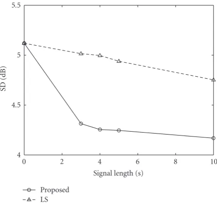
Figure 4 shows the RASTI score averaged over the 10 speakers’ results as a function of the length of the observed signal.Figure 5shows the SD averaged over the results for all time frames and speakers. There was little difference between the results of the proposed algorithm and those of the LS-based algorithm when the length of the observed signal was above 10 seconds. Hence, we plot the results for observed sig-nals duration up to 10 seconds in Figures4and5to highlight the difference between the two algorithms. We can see that the proposed algorithm outperformed the algorithm based on the LS criterion especially when the observed signals were short.

We found that, among the 10 speakers, the dereverbera-tion performance for the male speakers was a bit better than that for the female speakers. This is probably because as-sumption (1) fits better for male speakers because the pitches

10 8

6 4

2 0

Signal length (s) 4

4.5 5 5.5

SD

(dB)

Proposed LS

Figure5: SD as a function of observed signal length.

0.6 0.5 0.4 0.3 0.2 0.1 0

Time (s) −60

−40 −20 0

Energ

y

(dB)

After Before 15 dB

Figure6: Energy decay curves of impulse responses before and after dereverberation.

of male speeches are generally lower than those of female speeches.

InFigure 6, we show examples of the energy decay curves of impulse responses before and after the dereverberation ob-tained by using an observed signal of five seconds. A clear re-duction in reflection energy can be seen; there was a 15 dB reduction in the reverberant energy 50 milliseconds after the arrival of the direct sound.

From the above results, we conclude that the proposed algorithm can estimate the inverse filter of the room acoustic system with a relatively short 3–5 second observed signal.

5. ALGORITHM USING HIGHER-ORDER STATISTICS

random variables is characterized by both their SOS and their HOS. Therefore, an algorithm based on the independence of {d(n)}is expected to realize a highly accurate inverse filter estimation because it fully uses the characteristics of the in-novations process specified by assumption (1).

Before presenting the algorithm, we formulate a theorem about the uniqueness of the estimates,{d(n)}, of the innova-tions{e(n)}. In this section, we also assume that

(i) the innovations {e(n)} have non-Gaussian distribu-tions,

(ii) the innovations{e(n)}satisfy the Lindeberg condition [24].

Under these assumptions, we have the following theorem.

Theorem 3. Suppose that variables{d(n)}are not determin-istic. If{d(n)}are statistically independent with non-Gaussian distributions, thend(n)is equalized withe(n)except for a pos-sible scaling and delay.

Proof. The proof is deferred toAppendix E.

By using Theorems1and3, it is clear that the inverse filters of the room acoustic system and the speech production system are uniquely identifiable.

In practice, the doubly-infinite inverse filterG(z) in (4) is approximated by theL-tap FIR filter as

y(n)= L

k=0

g(k)Tx(t−k). (41)

Unlike the SOS-based algorithm, we need not constrain the first tap weights as (18). Thus, we estimate{gm(k)}withk≥ 0 in this section.

5.1. Loss function

Let us represent the mutual information of random variables

ξ1,. . .,ξnbyI(ξ1,. . .,ξn). By using the mutual information as a measure of the interdependence of the random variables, we minimize the loss function defined asI(d(1),. . .,d(N)) with respect to{a(k,n)}and{gm(k)}under the constraint that instantaneous systems{1−A(z,n)}are minimum phase in a similar way to (19). The loss function can be rewritten as (seeAppendix F)

Id(1),. . .,d(N)= − N

n=1

Jd(n)+Kd(1),. . .,d(N),

(42)

where J(ξ) denotes the negentropy [25] of random vari-ableξ. The computational formula of the negentropy is given later. The negentropy represents the nongaussianity of a ran-dom variable. From (42), what we try to solve is formulated as

minimize {a(k,n)},{gm(k)}

− N

n=1

Jd(n)+Kd(1),. . .,d(N)

subject to1−A(z,n)being minimum phase.

(43)

By comparing (43) with (19), it is found that (43) exploits the negentropies of{d(n)}in addition to the correlatedness be-tween{d(n)}as a criterion. Therefore, we try not only to un-correlate outputs{d(n)}but also to make the distributions of{d(n)}as far from the Gaussian as possible.

5.2. Algorithm

As regards time variant filter 1−A(z,n), we again use ap-proximation (29). Then, we solve

minimize {ai(k)},{gm(k)}

− N

n=1

Jd(n)+Kd(1),. . .,d(N)

subject to1−Ai(z)being minimum phase

(44)

instead of (43).

Problem (44) is solved by the alternating variables method in a similar way to the algorithm in Section 4. Namely, we repeat the minimization of the loss function with respect to{ai(k)}for fixed{gm(k)}and minimization with respect to{gm(k)}for fixed{ai(k)}. However, since the loss function of (44) is very complicated, we derive a suboptimal algorithm by introducing the following assumptions found in our preliminary experiment.

(i) Given{gm(k)}, or equivalently, given y(n), the set of parameters{ai(k)}that minimizesK(d(1),. . .,d(N)) also reduces the loss function of (44).

(ii) Given{ai(k)}, the set of parameters{gm(k)}that min-imizes (−N

n=1J(d(n))) also reduces the loss function of (44).

With assumption (i), we again estimate{ai(k)}1≤k≤Pby applying LP to segment{y(n)}Ni≤n≤Ni+W−1, which is the

out-put ofG(z), for eachi. It should be remembered that we can obtain minimum-phase estimates of{1−Ai(z)}by using LP. Next, we estimate{gm(k)}for fixed{ai(k)}by maximiz-ing N_n=1J(d(n)) based on assumption (ii). By using the Gram-Charlier expansion and retaining dominant terms, we can approximate the negentropyJ(ξ) of random variableξ

as [26]

J(ξ) κ3(ξ)2 12υ(ξ)3 +

κ4(ξ)2

48υ(ξ)4, (45)

whereκi(ξ) represents theith order cumulant ofξ. Generally, the innovations of a speech signal have supergaussian dis-tributions whose third-order cumulants are negligible com-pared with its fourth-order cumulants. Therefore, we finally reach the following problem in the estimation of{gm(k)}:

maximize {gm(k)}1≤m≤M, 0≤k≤L

N

n=1 κ4

d(n)

υd(n)2

{ai(k)}={ai(k)}

subject to M

m=1 L

k=0

gm(k)2=1.

(46)

60 50 40 30 20 10 0

Signal length (s) 0.75

0.8 0.85 0.9 0.95 1

RASTI

sc

o

re

HOS SOS

Figure7: RASTI as a function of observed signal length.

scaleαarbitrarily. We use the gradient method to realize this maximization. By taking the derivative of the loss function of (46), we have the following algorithm:

gm(k)=gm(k)

+δ

T

i=1 4

d(n)24

×d(n)3vm,i(n−k)

d(n)22 −d(n)4_d(n)2_d(n)v

m,i(n−k)

,

gm(k)= gm(k)

M m=1

L

k=0gm(k)2 ,

(47)

where the averages are calculated for indicesNitoNi+W−1. Here, we have again used the assumption thatd(n) is station-ary within a single frame just as we did in the derivation of (36).

Remark 3. While we can easily estimate{ai(k)}and{gm(k)} with assumptions (i) and (ii), the convergence of the al-gorithm is not guaranteed because the assumptions may not always be true. We examine this issue experimentally. It is hoped that future work will reveal the theoretical back-ground to the assumptions.

5.3. Experimental results

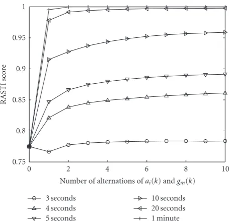
We compared the dereverberation performance of the HOS-based algorithm proposed in this section with that of the SOS-based algorithm described in the previous section. We used the same experimental setup as that in the previous sec-tion except for the iterasec-tion parametersR1andR2, which we set at 10 and 20, respectively.

Figure 7 shows the RASTI score averaged over the 10 speakers’ results as a function of the length of the observed

60 50 40 30 20 10 0

Signal length (s) 2.5

3 3.5 4 4.5 5 5.5

SD

(dB)

HOS SOS

Figure8: SD as a function of observed signal length.

10 8

6 4

2 0

Number of alternations ofai(k) andgm(k) 0.75

0.8 0.85 0.9 0.95 1

RASTI

sc

o

re

3 seconds 4 seconds 5 seconds

10 seconds 20 seconds 1 minute

Figure9: RASTI as a function of iteration number.

signal. As expected, we can see that the HOS-based algorithm outperformed the SOS-based algorithm when the observed signal was relatively long. In particular, when an observed signal of longer than 20 seconds was available, the RASTI score was nearly equal to one. Figure 8shows the average SD. Again, we can confirm the great superiority of the HOS-based algorithm to the SOS-HOS-based algorithm in terms of asymptotic performance.

Inf. 40

30 20

10

SNR (dB) 0.65

0.7 0.75 0.8 0.85 0.9 0.95 1

RASTI

sc

o

re

SOS, 5 seconds SOS, 20 seconds

HOS, 5 seconds HOS, 20 seconds

Figure10: RASTI obtained in the presence of noise.

of the RASTI score. The RASTI score converges particularly rapidly when the observed signal length is sufficiently large.

6. DISCUSSION

6.1. Effect of additive noise

Thus far, we have considered a system without any additive noise. In this section, we experimentally examine the effect of additive noise on the performance of the proposed algo-rithms3_.

We tested a case where the observed signal was con-taminated by additive white Gaussian noise with signal to noise ratios (SNR) of 40, 30, 20, and 10 dB. Since the pro-posed methods do not involve noise reduction, we mea-sured the performance as a RASTI score calculated by us-ing the impulse response of equalized room acoustic system G(z)T_H(z).

InFigure 10, we plot the average RASTI scores as a func-tion of the SNR for observed signals of five and twenty sec-onds. The SOS-based algorithm was relatively robust against additive noise. Although the performance of the HOS-based algorithm was degraded more severely than that of the SOS-based algorithm, the former still exhibited excellent perfor-mance in the presence of noise with an SNR of 30 dB or greater when the observed signal was 20 seconds long.

Thus, it is a promising way to combine the proposed algorithms with traditional noise reduction methods such as spectral subtraction [28] in a noisy environment with a

3_{We also conducted an experiment by using real recordings where the}

room acoustic system might fluctuate and where there was slight back-ground noise. Good dereverberation performance was achieved in this experiment. The result is reported in [27].

1 0.5 0 −0.5

−1 Realpart

−1 −0.5 0 0.5 1

Imag_inar y par_t

0 1 2 3 4 5 ×10−2

No

rm

al

iz

ed

n

u

m

b

er

of

app

ear

anc

e

Figure11: Histogram showing the number of poles of the speech

production system in each small region in the complex plane.

severe SNR. An investigation of such a combination is how-ever beyond the scope of this paper.

6.2. Validity of assumption (2)

Assumption (2) is one of the essential assumptions that form the basis of the proposed algorithms. Here we investigate its validity.

Figure 11is an example histogram showing the number of poles of the speech production system included in a clean speech signal of five seconds in each small region in the com-plex plane. The number of poles in each region is normalized by the total frame number. Due to this normalization, re-gions with a value of one correspond to time invariant poles. InFigure 11, we can see no such regions, which indicates that there is no time invariant pole. This result supports assump-tion (2).

7. CONCLUSION

We have described the problem of speech dereverberation. The contribution of this paper is summarized as follows.

(i) We proposed the joint estimation of the time invariant and time variant subfilters of the inverse filter of an overall acoustic system. It was shown that these subfil-ters correspond to the inverse filsubfil-ters of a room acoustic system and a speech production system, respectively. (ii) We developed two distinct algorithms; one uses a

crite-rion based on the SOS of the output while the other is based on the HOS. The SOS-based algorithm improves RASTI by 0.1 even when the observed signals are at most 5-second long. By contrast, the HOS-based algo-rithm estimates the inverse filter with a RASTI score of nearly one, as long as observed signals of longer than 20 seconds are available.

investigated practical issues such as computational costs and adaptation to time varying environments. A simple way to cope with these issues would be to employ stochastic gradi-ent learning. An exaustive subjective listening test should also be conducted. Investigating these issues in depth is a subject for future study.

APPENDICES

A. PROOF OFTHEOREM 1

By using (2), (5), and (13), we obtain

d(n)=1−A(z,n)G(z)TH(z)s(n). (A.1) Substituting (15) into (A.1) yields

αe(n−β)=1−A(z,n)G(z)TH(z)s(n). (A.2) On the other hand, from (9), we have

e(n)=1−B(z,n)s(n)=1−B(z,n)z−β_s(n+β). (A.3)

This equation is equivalent to

e(n−β)=1−B(z,n−β)z−β_{s(n). (A.4)} Relations (A.2) and (A.4) give

1−A(z,n)G(z)TH(z)

=1−B(z,n−β)αz−β_{, 1≤ ∀n≤N.} (A.5) Since both 1−A(z,n) and 1−B(z,n) have no time invariant zero according to (16) and (11), we have

G(z)T_H(z)=αz−β_{. (A.6)}

B. DERIVATION OF(26)

In this appendix, we show that log|detΣ(d)| is in-variant with respect to {a(k,n)}1≤n≤N, 1≤k≤P and {gm(k)}1≤m≤M, 1≤k≤L. We here assume that s(n) = 0 whenn ≤ 0. Hence, relation (B.10), which we derive here, may be an approximation.

Output vectord, defined by (25), is represented by using y=[y(N),. . .,y(1)]T _as

d=Ay, (B.1)

whereAis defined as (B.2): A= ⎡ ⎢ ⎢ ⎢ ⎢ ⎢ ⎢ ⎢ ⎢ ⎢ ⎢ ⎢ ⎢ ⎢ ⎢ ⎢ ⎢ ⎢ ⎢ ⎢ ⎢ ⎢ ⎢ ⎢ ⎢ ⎢ ⎣

1−a(1,N) · · · · · · −a(P,N)

1 −a(1,N−1)· · · · −a(P,N−1)

. ._. . ._.

1 −a(1,P+1) · · · · · · −a(P,P+1)

1 −a(1,P) · · · −a(P−1,P)

. ._. . ._. .._.

1 −a(1, 2)

1 ⎤ ⎥ ⎥ ⎥ ⎥ ⎥ ⎥ ⎥ ⎥ ⎥ ⎥ ⎥ ⎥ ⎥ ⎥ ⎥ ⎥ ⎥ ⎥ ⎥ ⎥ ⎥ ⎥ ⎥ ⎥ ⎥ ⎦ . (B.2)

RelationΣ(d) = E{ddT_{} = AE{yy}T_}AT _{= AΣ(y)A}T leads to

logdetΣ(d)=logdetΣ(y)+ 2 log|detA|. (B.3) Because the determinant of an upper triangular matrix is the product of its diagonal components, we have detA=1. Hence, we obtain

logdetΣ(d)=logdetΣ(y). (B.4) yis related tos=[s(N),. . .,s(1)]T_as

y= M

m=1

Gmxm=

_M

m=1 GmHm

s, (B.5)

wherexm,Gm, andHmare written as

xm=xm(N),. . .,xm(1)T,

Gm=

⎡ ⎢ ⎢ ⎢ ⎢ ⎢ ⎢ ⎢ ⎢ ⎢ ⎣

gm(0) · · · gm(L) O

. .. . ..

gm(0) · · · gm(L) . .. .._.

O gm(0)

⎤ ⎥ ⎥ ⎥ ⎥ ⎥ ⎥ ⎥ ⎥ ⎥ ⎦ ,

Hm=

⎡ ⎢ ⎢ ⎢ ⎢ ⎢ ⎢ ⎢ ⎢ ⎢ ⎣

hm(0) · · · hm(K) O

. .. . ..

hm(0) · · · hm(K) . .. .._.

O hm(0)

⎤ ⎥ ⎥ ⎥ ⎥ ⎥ ⎥ ⎥ ⎥ ⎥ ⎦ . (B.6)

Hence, in a similar way to (B.3), we obtain

logdetΣ(y)=logdetΣ(s)+ 2 logdet

_M

m=1 GmHm

=2 logdet

_M

m=1 GmHm

+ constant.

(B.7)

Since M_m=1GmHm is also an upper triangular matrix with diagonal elements ofM_m=1hm(0)gm(0), we have

logdet

_M

m=1 GmHm

=Nlog

_M

m=1

hm(0)gm(0)

.

(B.8)

Substituting (18) into (B.8) yields

logdet

_M

m=1 GmHm

=Nlogh1(0)= constant. (B.9)

By using (B.3), (B.7), and (B.9), we can derive

C. PROOF OFTHEOREM 2

By (4) and (12),d(n) is written by using{s(n−k)}0≤k≤K+L+P as

d(n)=h1(0)s(n) +Lc

s(n−k); 1≤k≤K+L+P, (C.1)

whereLc{·}stands for the linear combination. By substitut-ing (8) into (C.1),d(n) is rewritten as

d(n)=h1(0)e(n) +u

n;G(z),A(z,n), (C.2)

whereu(n) is of the form

u(n)=Lc

s(n−k); 1≤k≤K+L+P. (C.3)

Becauses(n) is of the form

s(n)=Lc

e(n),s(n−k); 1≤k≤P (C.4)

as in (8),s(n) has no components of{e(n+k)}k≥1. Therefore, e(n) andu(n) are statistically independent. Then, we have

υd(n)=h1(0)2υ

e(n)+υu(n)≤h1(0)2υ

e(n) (C.5)

with equality if and only if

υu(n)=0. (C.6)

Because the logarithmic function is increasing monotoni-cally,Nn=1logυ(d(n)) reaches a minimum if and only if

υu(n)=0, 1≤ ∀n≤N. (C.7)

According to (C.2), condition (C.7) is satisfied if and only if

d(n) is equalized withe(n) as

d(n)=h1(0)e(n). (C.8)

D. DERIVATION OF(36)

By using the assumption thatd(n) is stationary within a sin-gle frame and replacing the varianceυ(d(n)) by its sample estimate, the loss function of (33),Nn=1logυ(d(n)), is esti-mated by

T

i=1

Wlogd(n)2Ni+W−1

n=Ni ∝

T

i=1

logd(n)2Ni+W−1

n=Ni . (D.1)

The derivative of the right-hand side of (D.1) with respect to

gm(k) is

∂ ∂gm(k)

T

i=1

logd(n)2Ni+W−1

n=Ni

= T

i=1

2

d(n)2Ni+W−1

n=Ni

d(n)∂d(n)

∂gm(k)

!Ni+W−1

n=Ni .

(D.2)

The derivative ofd(n) belonging to theith frame is

∂d(n)

∂gm(k)=

∂y(n)

∂gm(k)− P

l=1

ai(l)∂y(n−l)

∂gm(k)

=xm(n−k)− P

l=1

ai(l)xm(n−l−k)

=vm,i(n−k).

(D.3)

From (D.2) and (D.3), we have the update equation of (36).

E. PROOF OFTHEOREM 3

Let{f(k,n)}−∞≤k≤∞ be the impulse response of the global system (1−A(z,n))G(z)T_{H(z)/(1−B(z,n)) at timen. Since}

d(n) has a non-Gaussian distribution, sequence{f(k,n)}has finite nonzero components according to the central limit the-orem [24]. Becaused(n) is not deterministic,{f(k,n)}has at least one nonzero component. Let the first nonzero compo-nent of{f(k,n)}be f(βn,n). Since the time variant part of the global system (1−A(z,n))G(z)T_{H(z)/(1−B(z,n)) has} the first tap of weight one, we have

βm=βn, f

βm,m= fβn,n, ∀m,∀n. (E.1) So we can represent the index and value of the first nonzero component asβandα, respectively. Because variables{d(n)} are independent, we obtain the following relation by using Darmois’ theorem [25]:

f(k,n)f(k−m,n−m)=0, ∀n,∀k, ∀m=0. (E.2)

If

k=β+m, (E.3)

we have

Therefore, ifm=0, we obtain by using (E.2)

f(k,n)= f(β+m,n)=0. (E.5)

Thus,{f(k,n)}has only one nonzero component f(β,n)=

α. Sinced(n) is represented as

d(n)=

"

1−A(z,n)G(z)T_H(z) 1−B(z,n)

#

e(n), (E.6)

d(n) is equalized withe(n) up to constant scaleαand delay

β.

F. DERIVATION OF(40)

Mutual informationI(d(1),. . .,d(N)) is defined as

Id(1),. . .,d(N)= N

n=1

Hd(n)−H(d), (F.1)

whereH(ξ) represents the differential entropy of (multivari-ate) random variableξ. From (B.1), we have

H(d)=H(y) + log|detA|. (F.2) Because of (B.3), we also have

log|detA| = 1 2

logdetΣ(d)−logdetΣ(y). (F.3) Substituting (F.2) and (F.3) into (F.1) gives

Id(1),. . .,d(N)

= N

n=1

Hd(n)−1

2logdetΣ(d)

+1

2logdetΣ(y)−H(y)

= − N

n=1

1 2logυ

d(n)−Hd(n)

+1 2

N

n=1

logυd(n)−logdetΣ(d)

+1

2logdetΣ(y)−H(y).

(F.4)

Now, the negentropy ofn-dimensional random variableξis defined as

J(ξ)=Hξgauss_−H

(ξ)

=1

2logdetΣ

ξgauss

+n

2(1 + log 2π)−H(ξ), (F.5)

whereξgaussis a Gaussian random variable with the same co-variance matrix as that ofξ. By using (20) and (F.5), (F.4) is rewritten as

Id(1),. . .,d(N)

= − N

n=1

Jd(n)+J(y) +Kd(1),. . .,d(N).

(F.6)

Furthermore, sinceyis related tosby anN×Nregular lin-ear transformation according to (B.5), and the negentropy is conserved by such linear transformation, we obtain

J(y)= constant. (F.7)

From (F.6) and (F.7), we finally reach (42).

REFERENCES

[1] L. R. Rabiner and R. W. Schafer,Digital Processing of Speech Signals, Prentice-Hall, Upper Saddle River, NJ, USA, 1983. [2] M. I. Gurelli and C. L. Nikias, “EVAM: an eigenvector-based

algorithm for multichannel blind deconvolution of input col-ored signals,”IEEE Transactions on Signal Processing, vol. 43, no. 1, pp. 134–149, 1995.

[3] K. Furuya and Y. Kaneda, “Two-channel blind deconvolution of nonminimum phase FIR systems,”IEICE Transactions on Fundamentals of Electronics, Communications and Computer Sciences, vol. E80-A, no. 5, pp. 804–808, 1997.

[4] S. Gannot and M. Moonen, “Subspace methods for multimi-crophone speech dereverberation,”EURASIP Journal on Ap-plied Signal Processing, vol. 2003, no. 11, pp. 1074–1090, 2003. [5] T. Hikichi, M. Delcroix, and M. Miyoshi, “Blind dereverbera-tion based on estimates of signal transmission channels with-out precise information on channel order,” inIEEE Interna-tional Conference on Acoustics, Speech, and Signal Processing (ICASSP ’05), vol. 1, pp. 1069–1072, Philadelphia, Pa, USA, March 2005.

[6] M. Delcroix, T. Hikichi, and M. Miyoshi, “Precise dereverber-ation using multichannel linear prediction,”IEEE Transactions Audio, Speech and Language Processing, vol. 15, no. 2, pp. 430– 440, 2007.

[7] B. Yegnanarayana and P. S. Murthy, “Enhancement of rever-berant speech using LP residual signal,”IEEE Transactions on Speech and Audio Processing, vol. 8, no. 3, pp. 267–281, 2000. [8] B. W. Gillespie, H. S. Malvar, and D. A. F. Florˆencio, “Speech

dereverberation via maximum-kurtosis subband adaptive fil-tering,” inIEEE Interntional Conference on Acoustics, Speech, and Signal Processing (ICASSP ’01), vol. 6, pp. 3701–3704, Salt Lake, Utah, USA, May 2001.

[9] B. W. Gillespie and L. E. Atlas, “Strategies for improving au-dible quality and speech recognition accuracy of reverberant speech,” inIEEE International Conference on Accoustics, Speech, and Signal Processing (ICASSP ’03), vol. 1, pp. 676–679, Hong Kong, April 2003.

[10] N. D. Gaubitch, P. A. Naylor, and D. B. Ward, “On the use of linear prediction for dereverberation of speech,” in Pro-ceedings of International Workshop on Acoustic Echo and Noise Control (IWAENC ’03), pp. 99–102, Kyotp, Japan, September 2003.

[11] T. Nakatani, K. Kinoshita, and M. Miyoshi, “Harmonicity-based blind dereverberation for single-channel speech sig-nals,”IEEE Transactions, Audio, Speech and Language Process-ing, vol. 15, no. 1, pp. 80–95, 2007.