Volume 2010, Article ID 617325,13pages doi:10.1155/2010/617325
Research Article
Distortion Analysis Toolkit—A Software Tool for Easy Analysis of
Nonlinear Audio Systems
Jyri Pakarinen
Department of Signal Processing and Acoustics, School of Science and Technology, Aalto University, P.O. Box 13000, 00076 Aalto, Finland
Correspondence should be addressed to Jyri Pakarinen,[email protected]
Received 27 February 2010; Revised 30 April 2010; Accepted 17 May 2010
Academic Editor: Udo Zoelzer
Copyright © 2010 Jyri Pakarinen. This is an open access article distributed under the Creative Commons Attribution License, which permits unrestricted use, distribution, and reproduction in any medium, provided the original work is properly cited.
Several audio effects devices deliberately add nonlinear distortion to the processed signal in order to create a desired sound. When creating virtual analog models of nonlinearly distorting devices, it would be very useful to carefully analyze the type of distortion, so that the model could be made as realistic as possible. While traditional system analysis tools such as the frequency response give detailed information on the operation of linear and time-invariant systems, they are less useful for analyzing nonlinear devices. Furthermore, although there do exist separate algorithms for nonlinear distortion analysis, there is currently no unified, easy-to-use tool for rapid analysis of distorting audio systems. This paper offers a remedy by introducing a new software tool for easy analysis of distorting effects. A comparison between a well-known guitar tube amplifier and two commercial software simulations is presented as a case study. This freely available software is written in Matlab language, but the analysis tool can also run as a standalone program, so the user does not need to have Matlab installed in order to perform the analysis.
1. Introduction
Since the 1990s, there has been a strong trend in the digital audio effects community towards virtual analog modeling, that is, mimicking the sound of old analog audio devices using digital signal processing (DSP). Guitar tube amplifier emulation [1] has been an especially vibrant area of research with several commercial products.
There are roughly two methodological approaches for designing virtual analog models: the black-box- and the white-box methods. In the former, the designer treats the original audio device (called target in the following) as an unknown system and tries to design the model so that it mimics only the input/output relationship of the target, without trying to simulate its internal state. In the white-box approach, the designer first studies the operation logic of the device (often from the circuit schematics) and tries to design the model so that it also simulates the internal operation of the target. While both approaches can yield satisfactory results in many cases, there is still room for improvement in the sound quality and model adjustability, if the virtual
analog models are to act as substitutes for the original analog devices.
In all virtual analog modeling, the target and model responses need to be carefully analyzed. This is obviously essential in the black-box approach, but it is also an unavoidable step in white-box modeling, since even circuit simulation systems need to have their component values adjusted so that the model response imitates the target response. While some part of this analysis can be conducted simply by listening to the models, there is a clear need for objective analysis methods. If the target system can be considered linear and time invariant (LTI), it is rela-tively straightforward to analyze the magnitude and phase responses of the target and model and try match them as closely as possible. For distorting systems, however, linear magnitude and phase responses give only partial information on how the system treats audio signals, since distortion components are not analyzed.
sine signal is fed to the system as an input, and the harmonic distortion component levels are summed and normalized to the amplitude of the fundamental component. Even though THD gives a vague indication on the general amount of static harmonic distortion, it tells nothing on the type of this distortion. Thus, THD is a poor estimate for analyzing distorting audio effects. Although more informative analysis techniques have been designed by the scientific community, there is currently no unified, easy-to-use tool for simultane-ously conducting several distortion analysis measurements.
2. Distortion Analysis Toolkit
2.1. Overview. The distortion analysis toolkit (DATK) is a
software tool for analyzing the distortion behavior of real and virtual audio effects. It operates by first creating a user-defined excitation signal and then analyzes the responses from the devices. The DATK package includes five analysis techniques, which can be further augmented with additional user-defined analysis functions. The DATK is developed in Matlab language, but standalone operation is also possible. Since a distortion measurement on an audio effects device usually consists of making several individual recordings while varying some control parameter and keeping the other parameters fixed, the DATK is designed for batch processing. This means that the DATK creates an excitation signal as an audio file according to the specifications set by the user. Next, the user plays this excitation to the device under test (DUT) and records the output on any playback/recording software. The DUT response to its control parameter variations can be tested by changing the control parameter values and rerecording the response. As a result, the user is left with a set of response files that each have different control parameter settings.
The analysis part is carried out by pointing the excitation file and the set of response files to the DATK, after which it plots analysis figures, so that each analysis type is shown as a separate figure, and the analysis results from each response file are illustrated with subfigures. Thus, it is easy to interpret the effect of control parameter variations on the system response, since each subfigure shows the response to a different value of the varied parameter. The analysis figures can also be saved as.fig files even in standalone mode, allowing further editing with Matlab. The DATK runs on any modern computer, and only requires the use of a simple playback/recording software for playing the excitation signal and recording the responses. For measuring software plugins, the playback/recording software should be able to act as a plugin host. For measuring physical effects devices, an audio interface with adjustable play-back/recording gains should be used. Sections2.2 through
2.6 discuss the analysis functions currently included in the DATK, while Section 2.7 discusses how to develop additional analysis functions. Since the user defines the desired analysis techniques and their parameters by writing a text file, where the different analysis types (or same analysis types with different parameters) are written as separate lines, Sections 2.2 through2.6 also introduce the syntax for performing each analysis type. The actual use of
the DATK software is illustrated in Section 3 with a case study.
2.2. Sine Analysis. One of the simplest distortion analysis
techniques is to insert a single sinusoid signal with fixed amplitude and frequency into the system, and plot the resulting spectrum. The advantage of this analysis type is that it is easy to understand and the results are straightforward to interpret. The disadvantage is that this analysis gives only information on how the system treats a single, static sine signal with given amplitude and frequency. In particular, it tells nothing about the dynamic behavior of the system. The DATK sine analysis function is invoked using the syntax
SineAnalysis(frequency,duration)
where thefrequencydenotes the frequency of the analysis sine in Hertz, and duration is the signal duration in seconds. The amplitude of the sine is set to unity. In the analysis phase, the DATK plots the resulting system response spectrum in the audio frequency range so that the amplitude of the fundamental frequency component (i.e., the component at the same frequency as the analysis sine) is 0 dB. The fundamental component is further denoted with a small circle around its amplitude peak, which helps in locating it if the spectrum has high-amplitude distortion components at subharmonic- or otherwise low frequencies.
2.3. Logsweep Analysis. The logsweep analysis technique is an
ingenious device for analyzing static harmonic distortion as a function of frequency. Introduced by Farina in 2000 [2], the basic idea behind the logsweep analysis technique is to insert a logarithmic sine sweep signal with fixed amplitude to the system, and then convolve the time-reversed and amplitude weighted excitation signal with the system response. As a result, one obtains an impulse response signal, where the response of each harmonic distortion component is separated in time from the linear response and each other. If the duration of the logsweep signal is long enough, the time separation between the harmonic impulse responses is clear and it is straightforward to cut the individual harmonic responses and represent them in the frequency domain. As a result, one obtains magnitude response plots for the linear response and each harmonic distortion component.
The DATK logsweep analysis function uses the syntax
LogsweepAnalysis(start freq,end freq,
duration,number of harmonics)
where start freq and end freq are the frequency limits (in Hz) for the logarithmic sweep, and duration
is the sweep duration in seconds. The parameter
(e.g.,>6), unless long excitation signals (several seconds) are used.
In the analysis phase, the DATK plots the linear and harmonic distortion component magnitude responses as a function of frequency (in the frequency range from
start freq to end freq) in a single figure. The response curves are illustrated with different colors and each curve has a number denoting the harmonic order, starting from 1 for the linear response, 2 for the 2nd harmonic, and so forth. The magnitude offset of the responses is set so that the magnitude of the linear response is 0 dB at low frequencies. The magnitude responses of the harmonic distortion components are shifted down in frequency by the order of their harmonic number. This means that looking at the analysis figure at a given frequency, say at 1 kHz, curve 1 gives the magnitude of the linear component, curve 2 gives the magnitude of the 2nd harmonic (which actually has the frequency of 2 kHz), curve 3 gives the magnitude of the 3rd harmonic (residing at 3 kHz), and so forth. This will be further illustrated in Section 3.6. The harmonic impulse responses are windowed using a Blackman window prior to moving them into the frequency domain, for obtaining smoother magnitude response plots [3].
The advantage of this measurement technique over the sine analysis (Section 2.2) is that it displays more informa-tion in a single figure by drawing the magnitude responses as a function of the (fundamental) frequency on the full audio frequency range. For analyzing the magnitude of high-order distortion components, however, the sine analysis is usually better since it displays the entire audible spectrum in one figure, while the logsweep analysis can successfully be used to track only the low-order distortion components, due to clarity reasons and the aforementioned SNR issue. Another drawback of the logsweep analysis technique is that long excitation signals can take a long time to analyze due to the relatively slow computation of long convolutions.
2.4. Intermodulation Distortion Analysis. When a multitone
signal is clipped, intermodulation distortion (IMD) occurs. This means that the distortion creates signal components not only to the integer multiples of the original tones, but also to frequencies which are the sums and differences of the original signal components and their harmonics. In musical context, IMD is often an undesired phenomenon, since IMD components generally fall at frequencies which are not in any simple harmonic relation to the original tones, making the resulting sound noisy and inharmonic.
Traditionally, the IMD of distorting systems has been measured by feeding a sum of two sinusoids with different frequencies into the system and plotting the resulting spectrum. Although this type of analysis gives an exact indi-cation of the frequencies and amplitudes of the distortion components for a given pair of input signal frequencies and amplitudes, it is not very useful in determining the overall level of the IMD. It should be noted that with distorting audio effects, it is often useful to know the exact frequency and amplitude behavior of the harmonic distortion compo-nents, since there are some strong opinions regarding the
harmonic content and the resulting sound, such as “the vacuum tube sound consists mainly of even harmonics”, or that “the 7th harmonic is something to be avoided”. With IMD, however, it is probably more useful to have a single number indicating the overall amount of distortion, since IMD is generally considered an undesired phenomenon, with no specific preferences on any particular IMD components. Furthermore, traditional IMD measurements ignore the dynamic behavior of the intermodulation mechanism, so that dynamic or transient intermodulation (DIM/TIM) [4] distortion components are left unnoticed.
The IMD analysis of the DATK software is based on the measurement technique introduced by Leinonen et al. [5], which measures both the DIM distortion and static IMD. In this measurement approach, a square wave signal with a fundamental frequency f1 is summed with a
lower-amplitude sinusoid having a frequency f2, so that f1 <
f2. Next, this signal is inserted to the DUT, and the
amplitude of the IMD components at audio frequency range is compared to the amplitude of the sinusoid. As a result, a percentage ratio between the root-mean-square (RMS) IMD components and the low-amplitude sinusoid riding on top of the square wave is obtained. Thus, an IMD percentage value of 100 % would mean that the RMS IMD is equal in magnitude to the frequency component that causes the IMD in the first place. The static IMD is measured in a very similar way, the only difference being that instead of a square wave signal, a triangular waveform is used.
For measuring the IMD, the DATK creates two signals: one containing the square wave and the sine wave (for measuring DIM), and one containing the triangle wave and the sine (for measuring static IM). In order to estimate the IMD as a function of input signal amplitude, both of these signals are weighted by a linear amplitude ramp, so that the overall signal amplitude increases with time, although the amplitude ratios between the square (or triangle) wave and the sine wave remain unchanged. The DATK IMD analysis is called with the function
IMDAnalysis(sine freq,sq freq,sine ampl,
sq ampl,duration)
where sine freq andsine ampl are the frequency (Hz) and amplitude of the sinusoid, respectively, and sq freq
andsq amplare the fundamental frequency and amplitude of the square wave. The triangle wave uses the same frequency and amplitude parameters as the square wave. The frequencies of the sine and square waves should be selected so that they are not in an integer relation with each other or the sampling frequency of the system.
output spectra for the IMD test signals and evaluates the DIM and IM percentages.
The advantage of the IMD measurement suggested in [5] over the traditional IMD measurements (i.e. simply plotting the output spectra), is that it provides two intuitive parameters concerning the IMD level: the IM percentage, which tells the amount of IMD associated with relatively static signals (such as the sound of a violin), and the DIM percentage, which tells the amount of IMD associated with transient signals (such as the sound of percussions).
2.5. Transient Response Analysis. Measuring the transient
behavior of distorting audio devices is difficult in general. Typically, the transient response depends heavily on the amplitude and frequency content of the test signal, so it is usually not possible to generalize the results for other types of input signals. Nevertheless, it is still useful to compare the input/output waveforms of a distorting device when a transient signal is used as input, for example because certain types of dynamic distortion (such as the blocking distortion, as in [7]) can be identified from the waveforms.
The DATK transient response analysis operates by creat-ing a sine burst signal, where the first cycle (called transient) has a larger amplitude than rest of the sine burst (called tail). The DATK transient response analysis function uses the syntax
TransientAnalysis(tail ampl,freq,
duration,cycles to draw)
where tail ampl denotes the amplitude of the tail of the sine burst following the transient, and should be a positive number smaller than one (the amplitude of the transient is always unity). Parametersfreqandduration
set the frequency (Hz) and duration (sec) of the sine burst, respectively. The parametercycles to drawsets the initial zoom limit in the analysis figure, so that dynamic distortion effects are easy to see. For example, a value of 10 would result in a waveform analysis figure, where 10 cycles of the response wave were displayed. The optimal value for thecycles to drawparameter obviously depends on the dynamic distortion characteristics of the device. If the DUT acts only as a static nonlinearity, the amplitude envelope, horizontal offset, and shape of the tail should remain constant in the analysis figure.
2.6. Aliasing Analysis. The DATK also has a tool for
estimat-ing the effect of signal aliasing in digital distorting devices. Nonlinear distortion always expands the signal spectrum by creating harmonic (and other) distortion components. This is problematic in a digital implementation, since the dis-tortion components exceeding the Nyquist frequency (half the sampling rate) will alias back to the baseband, possibly resulting in an inharmonic and noisy signal. There are several techniques for avoiding aliasing within digital distortion [1], oversampling being probably the most popular.
The aliasing analysis tool in the DATK operates by creat-ing a high-frequency sine signal, and analyzcreat-ing the spectrum of the system response. This analysis technique, introduced
Figure1: The custom-built AC30 tube guitar amplifier (photo by Ari Viitala).
in a recent journal article [7], tracks the nonaliased harmonic distortion components and fits a simple auditory spectrum curve on them, for estimating the frequency masking effect of the baseband signal. More specifically, the auditory spectrum curve is estimated by fitting a gammatone filterbank [8] magnitude response curve on top of the nonaliased signal so that the center frequencies of the filters are aligned with the frequencies of the baseband components. A fixed 10 dB offset between the peak of each sinusoidal signal component and the corresponding gammatone filter is applied since it was empirically found to match well with many distorted signals. Next, the effect of the hearing threshold is added by estimating the F-weighting function [9] for audio fre-quencies, together with a user-defined sound pressure level (SPL) value. The net effect of the masking curves and hearing threshold is obtained by taking the maximum value of the filter magnitude responses and theF-weighting function for each frequency.
Finally, the DATK creates a residual spectrum by removing the original sine and the nonaliased distortion components, and displays the residual spectrum in the same figure with the auditory spectrum estimate. Since the residual spectrum consists of the aliased signal components (and noise), one can assume that the aliasing artifacts (or noise) are audible, if the residual spectrum exceeds the auditory spectrum estimate in magnitude at any frequency. It should be noted that although there exist more sophisticated tech-niques (e.g., [10,11]) for estimating the auditory spectrum of complex tones, the use of a relatively simple auditory model in this context is enough to characterize the perceptual point of view. Evaluation in detail requires a detailed model compared against a careful formal listening test, which falls beyond the intended scope of the DATK tool.
The DATK aliasing analysis function is invoked by calling
AliasingAnalysis(freq,duration,SPL)
Figure2: Dialog box for creating the analysis signal.
Figure3: A dialog box for analyzing the system responses.
(in seconds), and the SPL parameter is the estimated F -weighted sound pressure level at which the distorted sine signal would be played.
2.7. Developing Additional Analysis Functions. The user can
append the DATK’s collection of analysis tools by developing
his or her own signal generation and analysis functions. Although the DATK can be operated as a standalone program, developing additional analysis tools requires the use of Matlab. Appending the DATK to include custom user-defined analysis tools is relatively simple, provided that the user is familiar with basic signal processing tasks on Matlab. The user-defined analysis tools should comply with some consistency rules, namely that
(i) there is a function for creating an excitation signal, possibly according to parameters set by the run-time user,
(ii) there is an analysis function which accepts a response signal and plots an analysis figure accordingly,
(iii) any additional parameters that the analysis function requires are generated as metadata by the excitation creation function and stored in a file.
More detailed instructions on developing custom analysis tools for DATK can be found on the DATK website:http:// www.acoustics.hut.fi/publications/papers/DATK/. After de-veloping the custom analysis tools, the user can easily com-pile a standalone version of the updated DATK using Matlab’s
deploytool-function.
3. Case Study: Measurement on the Real and
Virtual AC30 Guitar Amplifiers
This section illustrates the use of the standalone DATK software by measuring the distortion characteristics of an AC30 guitar tube amplifier and two of its virtual analog versions. The main purpose of this section is to provide an example case for producing distortion measurements using the DATK, rather than to perform a detailed interpretation of the operation of the devices. Thus, the emphasis is on explaining the measurement procedure, and what is the useful information in the analysis results, without trying to explain why the amplifier or its virtual versions have a certain effect on the signal.
3.1. VOX AC30. The AC30 is an iconic guitar tube amplifier,
first introduced by the VOX company in 1959 [13]. This class AB [14] amplifier uses four cathode-biased EL-84 tubes in the output stage. In 1961, a “Top Boost”-unit, an additional circuit box including treble and bass controls and an extra gain stage was introduced for the AC30. Due to its immediate popularity among users, the Top Boost unit was integrated into the AC30 circuitry from 1963 onwards. The distinct “jangly” sound of the AC30 amplifier can be heard on many records from several bands such as the Beatles, The Rolling Stones, The Who, Queen, R. E. M., and U2, from the last five decades.
−1
−0.5 0.5
0 1
0 1 7 8 9
×105
Figure4: Graphical user interface for manual alignment of the analysis signal.
were conducted on two commercial software emulators, namely the Top30 unit of the Overloud TH1 [15] plugin, and the FOX ACS-45 unit of the Peavey ReValver [16] plugin (abbreviated TH1 AC30 and ReValver AC30, resp., in the following).
3.2. Measurement Setup. The distortion behavior of the
real AC30 was measured with the DATK software running on a 2.4 GHz MacBook (Intel Core 2 Duo, 4 GB RAM) laptop computer with M-Audio Firewire 410 as the audio interface. The Reaper software [17] was used in playing the excitation and recording the responses. An 8Ω power resistor was used as a load for the amplifier. The amplifier output signal was obtained by recording the voltage over the load resistor using a custom-built attenuator/buffer circuit to eliminate the impedance coupling between the amplifier and the audio interface. It should be noted, that although real tube amplifiers usually require a separate attenuator/buffer circuit, many other distortion devices, such as effects pedals, may directly be connected to the audio interface. The high-impedance bright channel was used on the amplifier, and the tone knobs were all set to 12 o’clock. Different responses were measured by varying the “Volume bright” knob, which in practice controls the gain for the bright channel. On the software plugins also, the bright channel was selected (called “Brilliant” on the ReValver AC30), all tone controls were set to 12 o’clock, and different recordings were made while varying the channel gain. It should be noted that since the real AC30 was operated without a loudspeaker, the loudspeaker emulation was switched offfor both virtual plugins.
3.3. Creating the Analysis Signal. A complete analysis was
performed on the three systems. The five functions were stored in a text file, with the following parameter values:
SineAnalysis(1000,0.1),
TransientAnalysis(1/10,1000,2,20),
LogsweepAnalysis(20,20000,2,5),
IMDAnalysis(6000,1270,1,4,2),
AliasingAnalysis(5000,1,80),
This file was read during the analysis by DATK. Next, the excitation signal was created by double-clicking the
DATK Create program icon, which opens a dialog box illustrated in Figure 2. At step 1, a sampling frequency of 48000 Hz and a bit length equal to 24 were selected from the dialog box. A gap of 24000 samples (corresponding to half a second with the selected sample rate) was chosen between the individual excitations. The purpose of this segment of silence between the measurement signal bursts is to ensure that the different measurements do not affect each other, that is, that the previous response signal has faded before a new one begins. At step 2, the recently created text file was selected using the “Browse”-button, and at step 3, the name and path for the excitation file was selected. Finally, the “Create analysis signal”-button was pressed, resulting in a command-line message denoting that the excitation signal was successfully created.
3.4. Recording. The excitation signal was imported by the
−100 −50 0
A
m
plitude
(dB)
0 0.5 1 1.5 2
×104 Frequency (Hz)
Real AC30, low gain
(a)
−100 −50 0
A
m
plitude
(dB)
0 0.5 1 1.5 2
×104 Frequency (Hz)
TH1 AC30, low gain
(b)
−100 −50 0
A
m
plitude
(dB)
0 0.5 1 1.5 2
×104 Frequency (Hz)
ReValver AC30, low gain
(c)
−100 −50 0
A
m
plitude
(dB)
0 0.5 1 1.5 2
×104 Frequency (Hz)
Real AC30, middle gain
(d)
−100 −50 0
A
m
plitude
(dB)
0 0.5 1 1.5 2
×104 Frequency (Hz)
TH1 AC30, middle gain
(e)
−100 −50 0
A
m
plitude
(dB)
0 0.5 1 1.5 2
×104 Frequency (Hz)
ReValver AC30, middle gain
(f)
−100 −50 0
A
m
plitude
(dB)
0 0.5 1 1.5 2
×104 Frequency (Hz)
Real AC30, full gain
(g)
−100 −50 0
A
m
plitude
(dB)
0 0.5 1 1.5 2
×104 Frequency (Hz)
TH1 AC30, full gain
(h)
−100 −50 0
A
m
plitude
(dB)
0 0.5 1 1.5 2
×104 Frequency (Hz)
ReValver AC30, full gain
(i)
Figure5: Response spectra to a 1 kHz sinusoid for the real AC30 (left column), the Top30 unit of the TH1 software plugin (middle column), and the FOX ACS-45 unit of the ReValver software plugin (right column). The user adjustable gain knob was first set to 9 o’clock (top row), then to 12 o’clock (middle row), and finally to full (bottom row). As expected, the real AC30 has a higher noise floor than the digital versions.
the response directory contained 9 response signals as.wav files with sample rate of 48 kHz and 24-bit resolution.
3.5. Signal Analysis. The analysis part of the DATK was
started by double-clicking theDATK Analyze-program icon, which opens a dialog box illustrated in Figure 3. First, the wave file containing the excitation signal and the directory containing the response files were located using the “Browse” buttons at steps 1 and 2. The next pane, step 3, defines the type of time alignment between the excitation and response signals. The “Align manually” option, which allows the user to individually set the time alignment, was used. The other option allows the user to define a common delay (positive or negative) for all response files. A common delay value may be useful, for example if all responses
are obtained from the same device since the signal delay is typically identical between different responses. Since there were three versions of the AC30 with three gain settings each, three rows and three columns were selected at step 4 to display the nine analysis subfigures. Finally, the distortion analysis was started by pressing the “Analyze!” button.
−0.5 0 0.5
Output
0 0.005 0.01
Time (s) Real AC30, low gain
(a)
−0.5 0 0.5
Output
0 0.005 0.01
Time (s) TH1 AC30, low gain
(b)
−0.5 0 0.5
Output
0 0.005 0.01
Time (s) ReValver AC30, low gain
(c)
−0.5 0 0.5
Output
0 0.005 0.01
Time (s) Real AC30, middle gain
(d)
−0.5 0 0.5
Output
0 0.005 0.01
Time (s) TH1 AC30, middle gain
(e)
−0.5 0 0.5
Output
0 0.005 0.01
Time (s) ReValver AC30, middle gain
(f)
−0.5 0 0.5
Output
0 0.005 0.01
Time (s) Real AC30, full gain
Input Response
(g)
−0.5 0 0.5
Output
0 0.005 0.01
Time (s) TH1 AC30, full gain
Input Response
(h)
−0.5 0 0.5
Output
0 0.005 0.01
Time (s) ReValver AC30, full gain
Input Response
(i)
Figure6: Transient analysis waveforms for the real AC30 (left column), the TH1 AC30 (middle column), and the ReValver AC30 (right column). The input signal is illustrated with a dashed line, while the solid line denotes the measured response. The gain knob was first set to 9 o’clock (top row), then to 12 o’clock (middle row), and finally to full (bottom row).
the user has aligned all the responses with the excitation, the DATK begins the analysis calculation and draws the result figures in the order defined in the analysis command text file.
3.6. Results. Prior to performing the analysis using DATK,
the three AC30 variants were tested with an electric guitar. The output signals from all test cases were fed to headphones through a TH1 loudspeaker cabinet simulator in order to obtain a more natural electric guitar sound. This informal and highly subjective playing test revealed that the real AC30 had a certain “smooth” distortion type that was not entirely captured by either software plugins, although the TH1 AC30
managed to get closer to it than the ReValver AC30, which sounded somehow too “harsh”, especially when using full gain.
1 3 2 4 5 −60 −40 −20 0 M ag nitude (dB)
102 103 104
Frequency (Hz) Real AC30, low gain
(a) 1 2 3 4 5 −60 −40 −20 0 M ag nitude (dB)
102 103 104
Frequency (Hz) TH1 AC30, low gain
(b) 1 2 3 4 5 −60 −40 −20 0 M ag nitude (dB)
102 103 104
Frequency (Hz) ReValver AC30, low gain
(c) 1 2 3 4 5 −60 −40 −20 0 M ag nitude (dB)
102 103 104
Frequency (Hz) Real AC30, middle gain
(d) 1 2 3 4 5 −60 −40 −20 0 M ag nitude (dB)
102 103 104
Frequency (Hz) TH1 AC30, middle gain
(e) 1 2 3 4 5 −60 −40 −20 0 M ag nitude (dB)
102 103 104
Frequency (Hz) ReValver AC30, middle gain
(f) 1 2 3 4 5 −60 −40 −20 0 M ag nitude (dB)
102 103 104
Frequency (Hz) Real AC30, full gain
(g) 1 2 3 4 5 −60 −40 −20 0 M ag nitude (dB)
102 103 104
Frequency (Hz) TH1 AC30, full gain
(h) 1 2 3 4 5 −60 −40 −20 0 M ag nitude (dB)
102 103 104
Frequency (Hz) ReValver AC30, full gain
(i)
Figure7: Logsweep analysis of the real AC30 (left column), the TH1 AC30 (middle column), and the ReValver AC30 (right column). The gain knob was first set to 9 o’clock (top row), then to 12 o’clock (middle row), and finally to full (bottom row). The numbered curves represent the order of the distortion, so that curve 1 corresponds to the linear magnitude response, curve 2 to the 2nd order harmonic distortion, curve 3 to the 3rd order harmonic distortion, and so forth. The 6th order and higher distortion components are not illustrated.
Increasing the gain level to medium (middle row), the even harmonic components become more suppressed in the real AC30 response, while the overall spectral envelope gets brighter. The ReValver AC30 response seems to simulate this even-order distortion component attenuation well. Both virtual plugins show a slightly stronger lowpass-effect than the real AC30 with medium gain. For full gain settings, the even-order distortion components exceed the odd-order components in the real AC30 response. For the ReValver AC30, the opposite happens: the odd-order components are significantly louder. As expected, the overall spectral envelope gets even brighter with increased gain in all three AC30 variants. Looking at all responses inFigure 5, it seems that the spectrum of the real AC30 response varies strongly on the gain level and this change is more subtle with the software versions.
The second analysis type produces the transient response plot, illustrated inFigure 6, where the dashed line denotes the input signal, while the response waveform is drawn
with a solid line. The vertical axis has been zoomed in between−0.5–0.5 to better illustrate the dynamic effects. It can be seen in the figure that the initial transient is hard-clipped in nearly all cases. For low-gain settings (top row), the real AC30 shows a slight bias shift after the transient, without a strong effect on the waveform. The TH1 AC30 response experiences a slightly stronger bias shift, with a heavier distortion immediately after the transient, while the ReValver AC30 response is more static. For medium and full gain settings (middle and bottom row), the real AC30 shows a slight attenuation right after the transient, which might indicate blocking distortion [7]. The TH1 AC30 response shows an exaggerated bias shift due to the transient, while the ReValver AC30 response is again more static. With full gain, the real AC30 waveform is more severely distorted than with the software plugins.
0 50 100 150 200
DIM/IM
(%)
0 0.5 1
Input signal amplitude (normalized) Real AC30, low gain
(a)
0 50 100 150 200
DIM/IM
(%)
0 0.5 1
Input signal amplitude (normalized) TH1 AC30, low gain
(b)
0 50 100 150 200
DIM/IM
(%)
0 0.5 1
Input signal amplitude (normalized) ReValver AC30, low gain
(c)
0 50 100 150 200
DIM/IM
(%)
0 0.5 1
Input signal amplitude (normalized) Real AC30, middle gain
(d)
0 50 100 150 200
DIM/IM
(%)
0 0.5 1
Input signal amplitude (normalized) TH1 AC30, middle gain
(e)
0 50 100 150 200
DIM/IM
(%)
0 0.5 1
Input signal amplitude (normalized) ReValver AC30, middle gain
(f)
0 50 100 150 200
DIM/IM
(%)
0 0.5 1
Input signal amplitude (normalized) Real AC30, full gain
DIM IM
(g)
0 50 100 150 200
DIM/IM
(%)
0 0.5 1
Input signal amplitude (normalized) TH1 AC30, full gain
DIM IM
(h)
0 50 100 150 200
DIM/IM
(%)
0 0.5 1
Input signal amplitude (normalized) ReValver AC30, full gain
DIM IM
(i)
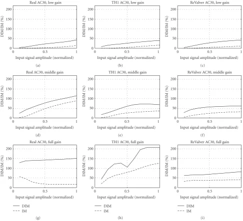
Figure8: Intermodulation distortion analysis of the real AC30 (left column), the TH1 AC30 (middle column), and the ReValver AC30 (right column). The gain knob was first set to 9 o’clock (top row), then to 12 o’clock (middle row), and finally to full (bottom row). The solid line illustrates the amount of dynamic intermodulation distortion, while the dashed line denotes the amount of static intermodulation distortion, both as a function of the normalized input signal level.
highpass behavior in the audio range as the real AC30, while the TH1 AC30 response is flatter. For low and medium-gain settings, the distortion components on the real AC30 have a highpass nature. The even harmonics on the TH1 AC30 mimic this somewhat, while the odd harmonics are more pronounced in the low frequencies than with the real AC30. The odd harmonics on the ReValver AC30 have a highpass trend for low and medium-gain, but the even harmonics are attenuated more than in the real AC30. For full gain, the second and third harmonics on the real AC30 are very strong at high frequencies. Neither software plugins have such a high distortion in the kilohertz range as the real AC30. Furthermore, neither plugins mimic the boosting of
the third harmonic and simultaneous suppression of the fifth harmonic at low frequencies (near 70 Hz).
The fourth analysis result created by the DATK is the intermodulation distortion analysis plot, illustrated in
−100 −50 0
A
m
plitude
(dB)
100 1 k 10 k
Frequency (Hz) Real AC30, low gain
(a)
−100 −50 0
A
m
plitude
(dB)
100 1 k 10 k
Frequency (Hz) TH1 AC30, low gain
(b)
−100 −50 0
A
m
plitude
(dB)
100 1 k 10 k
Frequency (Hz) ReValver AC30, low gain
(c)
−100 −50 0
A
m
plitude
(dB)
100 1 k 10 k
Frequency (Hz) Real AC30, middle gain
(d)
−100 −50 0
A
m
plitude
(dB)
100 1 k 10 k
Frequency (Hz) TH1 AC30, middle gain
(e)
−100 −50 0
A
m
plitude
(dB)
100 1 k 10 k
Frequency (Hz) ReValver AC30, middle gain
(f)
−100 −50 0
A
m
plitude
(dB)
100 1 k 10 k
Frequency (Hz) Real AC30, full gain
Signal Aud. spec. Aliasing
(g)
−100 −50 0
A
m
plitude
(dB)
100 1 k 10 k
Frequency (Hz) TH1 AC30, full gain
Signal Aud. spec. Aliasing
(h)
−100 −50 0
A
m
plitude
(dB)
100 1 k 10 k
Frequency (Hz) ReValver AC30, full gain
Signal Aud. spec. Aliasing
(i)
Figure9: Aliasing analysis for the real AC30 (left column), the TH1 AC30 (middle column), and the ReValver AC30 (right column), when a 5 kHz sine is used as input. The gain knob was first set to 9 o’clock (top row), then to 12 o’clock (middle row), and finally to full (bottom row). In the figures, the circles denote the peaks of the harmonic components, while the solid line stands for aliased signal components and noise. The dashed line illustrates an auditory spectrum estimate. In both software plugins (middle and right column), the aliased components greatly exceed the estimated auditory threshold, thus suggesting that the aliasing is clearly audible. For the real AC30 (left column), the figures show that the 50 Hz power supply hum and its harmonics are also audible.
With full gain (bottom row), however, the intermodulation distortion figures reveal stronger differences. On the real AC30, the static IM distortion decreases with increasing input signal amplitude, while the DIM distortion remains nearly constant. The TH1 AC30 shows an interesting notch in the DIM distortion curve, indicating that there could be a local minimum of DIM distortion with input signals with a certain amplitude. The DIM/IM distortion on the ReValver AC30 with full gain seems to be relatively low and largely unaffected by the input signal amplitude.
In general, it seems that there are no large differences in the intermodulation distortion behavior between the real and simulated AC30 variants at low- and medium
gain settings. However, the underlying mechanisms causing the different full-gain intermodulation distortion behavior between the AC30 variants should be examined in detail in further studies.
The fifth and final analysis plot is the aliasing analysis, depicted in Figure 9. It illustrates the estimated auditory spectrum (dashed line) caused by a distorted 5 kHz sine signal. The amplitude peaks of the distorted signal are plotted with circles. The solid lines in the figures illustrate the aliased signal components and measurement noise.
noise is clearly audible also in quiet parts when using the amplifier in a real playing situation. Interestingly, the aliasing analysis plots for both virtual AC30 plugins (second and third column) show severe aliasing phenomenon. The aliased component at 1 kHz is roughly 40 dB above the auditory spectrum estimate at full gain settings, making it clearly audible. In fact, the heavy aliasing behavior can strongly be heard also by listening to the logsweep responses of the AC30 plugins. It should be noted that the power supply noise is generally less irritating than aliasing noise, since the former stays largely constant regardless of the input signal. Aliasing noise, in turn, changes radically according to the input signal, and can it be an especially undesired phenomenon when playing high bent notes, since when the original tone moves up in frequency, the strongest aliased components move down, creating an unpleasant effect.
After all the analysis figures have been created, the DATK analysis part is finished. For the 2.4 GHz MacBook test computer, it took 76 seconds to analyze the AC30 responses (66 seconds when running under Matlab), while clearly most of the time is spent in performing the logsweep analysis.
4. Conclusion
A new software tool for performing rapid analysis measure-ments on nonlinearly distorting audio effects was presented. The software is called Distortion Analysis Toolkit (DATK), and it is freely available for download at http://www .acoustics.hut.fi/publications/papers/DATK/. The software operates by first creating an excitation signal as a.wav file according to the specifications set by the user. Next, the user feeds this excitation signal as an input to a physical or virtual distorting audio effect and records the output. Several recordings can be made if the distorting effect’s control parameter variations are to be analyzed. Finally, the introduced software analyzes the response files and displays the analysis results with figures. The software is developed in Matlab language, but it can also be operated in standalone mode. The DATK includes five distortion analysis methods, and additional analysis techniques can be appended to it using Matlab.
The usage of the DATK was illustrated with a case study, where a custom-built AC30 guitar tube amplifier and two commercial software simulations, TH1 AC30 and ReValver AC30, were measured and compared. The amount and type of distortion on the real AC30 were found to be strongly dependent on the channel gain, as well as input signal frequency. Especially the amplitude ratios between the first few harmonic components show a complex nonmonotonous dependency from the channel gain. Although both soft-ware plugins successfully simulate the overall distortion characteristics in a broad sense, their response is more static than the real AC30 response. Waveform responses to a transient input signal reveal that the nonlinearity in the real AC30 is dynamic. Also the tested TH1 AC30 plugin shows strong dynamic behavior, while the ReValver AC30 plugin is more static. Intermodulation distortion
analysis did not reveal any major differences between the three AC30 variants for low- and medium-gain settings, although some differences could be observed under full gain operation. Clearly audible aliasing noise was observed for both software plugins with sinusoid inputs when running a 48 kHz sample rate, whereas the real AC30 suffered from power supply hum. In a practical guitar playing condition, the aliasing noise on the tested software plugins is in most cases negligible due to the complex spectrum of the guitar. High bent notes can, however, reveal audible aliasing artifacts even when operating at a 96 kHz sample rate.
Acknowledgments
This research is funded by the Aalto University. The author is grateful to Vesa V¨alim¨aki for helpful comments. Special thanks are due to Ari Viitala for building the AC30 amplifier.
References
[1] J. Pakarinen and D. T. Yeh, “A review of digital techniques for modeling vacuum-tube guitar amplifiers,”Computer Music
Journal, vol. 33, no. 2, pp. 85–100, 2009.
[2] A. Farina, “Simultaneous measurement of impulse response and distortion with a swept-sine technique,” in Proceedings
of the 108th AES Convention, Paris, France, February 2000,
preprint 5093.
[3] P. D. Hatziantoniou and J. N. Mourjopoulos, “Generalized fractional-octave smoothing of audio and acoustic responses,”
Journal of the Audio Engineering Society, vol. 48, no. 4, pp. 259–
280, 2000.
[4] M. Otala, “Transient distortion in transistorized audio power amplifiers,”IEEE Transactions on Audio and Electroacoustics, vol. 18, no. 3, pp. 234–239, 1970.
[5] E. Leinonen, M. Otala, and J. Curl, “A method for measuring transient intermodulation distortion (TIM),” Journal of the
Audio Engineering Society, vol. 25, no. 4, pp. 170–177,
1977.
[6] V. V¨alim¨aki and A. Huovilainen, “Oscillator and filter algo-rithms for virtual analog synthesis,”Computer Music Journal, vol. 30, no. 2, pp. 19–31, 2006.
[7] J. Pakarinen and M. Karjalainen, “Enhanced wave digital triode model for real-time tube amplifier emulation,”IEEE
Transactions on Audio, Speech and Language Processing, vol. 18,
no. 4, pp. 738–746, 2010.
[8] R. D. Patterson, “The sound of a sinusoid: spectral models,”
Journal of the Acoustical Society of America, vol. 96, no. 3, pp.
1409–1418, 1994.
[9] R. A. Wannamaker, “Psychoacoustically optimal noise shap-ing,”Journal of the Audio Engineering Society, vol. 40, no. 7-8, pp. 611–620, 1992.
[10] K. Brandenburg, G. Stoll, Y. F. Deh´ery, J. D. Johnston, L. V. D. Kerkhof, and E. F. Schr¨oder, “The ISO-MPEG-1 audio: a generic standard for coding of high-quality digital audio,”
Journal of the Audio Engineering Society, vol. 42, no. 10, pp.
780–792, 1994.
[11] S. Van De Par, A. Kohlrausch, G. Charestan, and R. Heusdens, “A new psychoacoustical masking model for audio coding applications,” inProceedings of the IEEE International
Confer-ence on Acoustic, Speech, and Signal Processing, vol. 2, pp. 1805–
[12] S. Errede, “Measurement of the electromagnetic properties of electric guitar pickups,” Tech. Rep., February 2010, http:// online.physics.uiuc.edu/courses/phys498pom/lab handouts/ electric guitar pickup measurements.pdf.
[13] J. Elyea, “The history of Vox,” April 2010, http://www .voxamps.com/history.
[14] R. Aiken, “Is the Vox AC-30 really class A?” 2002,http://www .aikenamps.com/VoxAC30classA 2.html.
[15] “Overloud TH1,” February 2010,http://www.overloud.com/. [16] “Peavey ReValver,” February 2010, http://www.peavey.com/
products/revalver/index.cfm.