Signal restoration via a splitting approach

(1)

R E S E A R C H

Open Access

Signal restoration via a splitting approach

Bushra Jalil

*

, Eric Fauvet and Olivier Laligant

Abstract

In the present study, a novel signal restoration method from noisy data samples is presented and is termed as

“signal split (SSplit)” approach. The new method utilizes Stein unbiased risk estimate estimator to split the signal, the Lipschitz exponents to identify noise elements and a heuristic approach for the signal reconstruction. However, unlike many noise removal techniques, the present method works only in the non-orthogonal domain. Signal restoration was performed on each individual part by finding the best compromise between the data samples and the smoothing criteria. Statistical results are quite promising and suggest better performance than the

conventional shrinkage. Furthermore, the proposed method preserves the energy of the sharp peaks and edges which, is not however, the case for classical shrinkage methods.

Keywords:continuous wavelet transform, wavelet transform modulus maxima, split or segmentation, Stein unbiased risk estimate, thresholding, modulus maxima, Lipschitz exponent

1 Introduction

In the past two decades, wavelet transform has been used as significant non-parametric estimation tool to extract noise elements from the signal. Antoniadis et al provided an extensive review of the vast literature of wavelet shrinkage and wavelet thresholding estimator developed to denoise data [1]. Among these denoising techniques, the modulus maxima approach proposed by Mallat et al. has received the most attention in continu-ous and non-orthogonal domains [2,3]. Although many researchers have proposed different methods to estimate signals from the evolution of the wavelet transform modulus maxima (WTMM) across different scales [4-11], still the proposed reconstruction process are either complicated or computationally expensive. More recently, Chen at al. presented a neighboring coefficients based multi wavelets denoising method [12].

Another domain of denoising techniques studies on the principle of shrinkage [13]. The shrinkage method uses nonlinear thresholding approach to shrink the orthogonal wavelet coefficients as a denoising tool. This method relies on the idea that the energy of the func-tion is often concentrated in a few wavelet coefficients while the energy of the noise is spread over all coeffi-cients, therefore by selecting a suitable threshold value it

is possible to reduce a significant amount of noise ele-ments by using nonlinear thresholding in the wavelet domain [13]. However, the denoised signal in this case may contain spurious oscillations due to the translation variant property of the discrete wavelet transform. After-wards, several approaches were proposed to overcome these problems of shrinkage but so far none of them guarantees the preservation of edges or sharp variations possibly due to their working in an orthogonal basis [13-17]. Fodor and Kamath presented a brief survey of some of these approaches [17]. More recently, Blu and Luisier presented the state of the art SURE-LET method for image denoising [18]. The performance of the SURE-LET method is quite outstanding in the presence of Gaussian noise. In the present study, we are addres-sing only 1D signal therefore it is not possible to com-pare with the SURE-LET method. However in the future study, the extension of the proposed method for 2D cases will give logical comparison of the two methods.

The main motivation of the current study is to over-come the existing problems in the previously proposed methods and to preserve the transitions at a relatively lower computational cost without introducing any oscil-lations. The new technique worked on the idea of split-ting the signal. The method segments the signal based on the sharpness of its transitions. In this way, the main transitions presented inside the signal have been pre-served at the initial stage. This segmentation is * Correspondence: [email protected]

Le2i Laboratory, Université de Bourgogne, 12 Rue de la Fonderie, Le Creusot, France

(2)

performed by Stein’s unbiased risk estimate (SURE) based nonlinear thresholding of WTMM. Once the sig-nal has been split into different sub sigsig-nals, Lipschitz exponents were computed for all the significant transi-tions present inside each sub signal. These Lipschitz exponents permit to separate the regular or smooth points from the noise elements. At the final stage, signal reconstruction involves in finding the best compromise between the data points and the smoothness criterion. At the end, all sub signals were merged together to reconstruct the fully denoised signal.

The article is organized as follows. The principle of the method is given in Section 2. Section 3 explains the proposed splitting approach. The proposed noise removal technique for the subs signals and the recon-struction method is given in Section 4. Results and com-parative analysis of the SSplit method with the SURE Shrink method [13] is given in Section 5 and finally, Section 6 concludes the study. The summary of the method is given in Appendix section.

2 Principle of the method

The proposed method can be divided into two main stages: signal splitting and restoration. Suppose we have a noisy functionYsuch that:

Y=F(ti) +εi, where i= 1, ...,N (1)

F(ti) is the deterministic function with ti= (i-1)/N, N

is the total number of samples andiis white gaussian

noiseN(0,s2). The aim of the current study is to esti-mate the function F with the minimum mean square error (MSE). The MSE of an estimator_Fˆ with respect to the estimated parameterF. In this study, all MSE were computed between restored signal and original (noise free) signal. To estimate the functionF, the method pro-poses to split the functionY into its subsets in spatial domain based on the sharpness of transitions or edges such that:

Y⊇Yi=1,2,...,J (2)

Ydenotes the setof all samples and each subset Yi,

withi= 1, ...,J containsKi adjacent samplesyi,lwhere l

1, ...Ki.J is the total number of subset and Ki is the

length of each respective subset. Piecewise analysis was performed on each subset of the functionY. The selec-tion of subsets is defined by SURE based nonlinear thresholding of WTMM. Once the signal has been split into subsets, the WTMM approach was applied on each subset individually to compute the Lipschitz exponents of the transitions in each subset. These Lipschitz expo-nents identify the regular or smooth points in the signal. The nonlinear function is then optimized between all the regular points using an iterative method to restore

the signal from each subset. Finally, all subsets were merged together to reconstruct the fully denoised signal. Four different types of synthetic signals used in this study are taken from the work by Donoho et al.: blocks, bumps, heavisine and dopplers as shown in Figure 1.

3 Signal splitting method (SSplit)

In order to split the signal, continuous wavelet trans-form based multiscale analysis has been applied on sig-nal y(t) to compute the modulus maxima by using an integrable function [2,3]:

WT(u,s) = √1

s

+∞

−∞ y(t)∗

(t−u)

s

dt (3)

where WT(u, s) is the wavelet coefficient of the func-tion y(t),Ψ(t) is the analyzing wavelet, s(> 0) is the scale parameter and uis the position parameter. The Gaus-sian function (θ(t)) has an important property of contin-uous differentiability, which makes this function suitable for the analysis of most types of signals. Therefore, the derivative of the Gaussian function has been used as a wavelet analyzing function (Ψ(t)) for the splitting method. These WTMM computed by using the deriva-tive of the Gaussian wavelet is defined as any point (u0,

s0) such that∥Wf(u, s0)∥ has a local maximum atu =u0

[2,3].

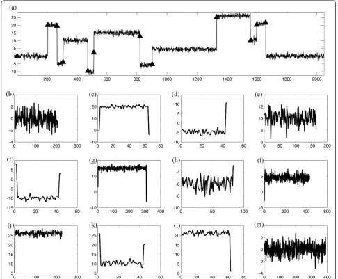
In order to select the optimum threshold criterion for making the subsets, the level-dependent thresholds are derived from modulus maxima by regarding the differ-ent scale levels as independdiffer-ent multivariate normal esti-mation problems. SURE gives an estimate of the risk for a particular threshold valuet; minimizing this in tgives a selection of the threshold level for that levelj(j= 1, 2 ...,J) [19]. SURE-based thresholding on modulus max-ima results in splitting the signal into subsets based on the sharpness of transitions. Figure 2 shows the thresh-olding results and respective splitting points on decom-posed signal. The first derivative of Gaussian function is used as a mother wavelet function on the block function with the sample size of 2048. Tracing these modulus maxima lines from coarser scales to finer scale gives the split edges at a convergence point on the finest scale. In short, a nonlinear soft thresholding at the decomposi-tion levelJ = 10 with the signal size of 2J results in giv-ing all the split points in block signal. In the present study, we termed the signal between two split points as a“subset”. Figure 3 shows the resulting subsets along with the split points obtained in the original block signal by applying SURE based nonlinear soft thresholding. In this section, we had explained the proposed splitting process and the coming sections will explain the noise

Jalilet al.EURASIP Journal on Advances in Signal Processing2012,2012:38 http://asp.eurasipjournals.com/content/2012/1/38

(3)

extraction method and the proposed reconstruction technique.

4 Singular points estimation and signal restoration

The second stage of the denoising algorithm deals with the extraction of noise elements from each individual subset. Mallat highlighted that the wavelet transform has a sequence of local maxima that converges to a point at a finer scale even though the function is regular at that point [2,3]. Therefore, in order to detect the

singularities it is not sufficient to follow the wavelet modulus maxima across scales. The Lipschitz exponents measure the regularity or singularity from the decay of these modulus maxima lines. By utilizing this property of Lipschitz exponents, the proposed method recon-structs the signal between all regular points using non-linear functions.

4.1 Modulus maxima lines and Lipschitz exponent Continuous wavelet transform based multiscale analysis was applied on each subsetYi(t) individually to compute Figure 1Four different synthetic signals used in this study.(a)Blocks,(b)bumps,(c)heavisine, and(d)dopplers.

(4)

the modulus maxima line. The modulus maxima line is any connected curveS(u) in the scale-space plane (u, s) along which all points are modulus maxima (Figure 4b). It has been shown by Mallat that the point wise singula-rities can be computed by measuring the decay of the slope of∥Wf(u, s)∥as a function oflog2(s) and is termed

as the Lipschitz exponent [2,3].

Definition 1 Supposenis an integer such that,n <a <n+ 1, the signal y(t) has Lipschitz aat t0, if and only

if there exists a constant A andt0> 0 and a polynomial

Pn(t) of ordern, such that fort<t0

y(t)−Pn(t)≤A|t−t0|α (4)

where the least upper bound ofa at the point oft0is

defined as the regularity of y(t) at the point of t0.

Lipschitz exponents can be computed from modulus

maxima lines by using Eq. (4). Lipschitz exponents actu-ally represent the nature of the signal in term of its dif-ferentiability and can be describe for a point or for interval as well. The scope of this study is limited to the study of point wise Lipschitz estimation. Figure 5 sum-marizes the results of Lipschitz estimation for different types of edges normally present inside the signal. In the case of Step function, Lipschitz exponent of 0 corre-spond to the discontinuity and also the function is non-differentiable as well. Similarly, impulse function is con-sidered to be as a singular and have negative Lipschitz estimation. In many situations, noise is also considered as an impulse in nature. Therefore, in more generalized way negative Lipschitz correspond to the noise elements. The more smoother regions have higher Lipschitz order and hence are differentiable more than once [2,3]. Figure 3Signal Splitting.(a)Signal with Gaussian white noise addition, proposed split points shown as arrow marks,(b)-(m)Subsets of noisy signal obtained with the first derivative of Gaussian function as a wavelet analyzing function.

(5)

4.2 Reconstruction method

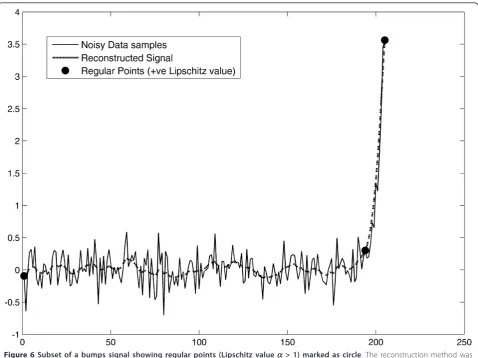
The present method proposes restoring each subset individually by taking into account extracted regular data samples based on their respective Lipschitz expo-nents as shown in Figure 6. These regular samples represent the smoother regions present inside the signal, therefore the reconstruction method does not change these data samples. The actual values at these points are preserved and the restoration is performed between these regular data samples. The restoration process was performed between two data samples and hence the first and last data samples have also been considered as regular data points.

The restoration method between regular data samples utilizes all sampled points and the smoothness of each subset to estimate the best fit. In the final stage, mer-ging of all reconstructed subsets result in giving fully denoised signal.

We define

Y_ik+1=Y_ik+λk_i

−∂C

MSE,k i ∂Yi

+γ_ik

−∂C

MSO,k i ∂Yi

(5)

Yidenotesi = 1, ...,Jsubsets withKiadjacent samples

(yi,l withl1, ...Ni).kdefine the iteration step.CMSE_i is

the mean square error estimation of the restored subset Figure 4Synthetic signal with the corresponding maxima lines.(a)Combination of synthetic signals: heavisine, bumps, blocks, and dopplers,(b)modulus maxima lines with the first derivative of Gaussian function as a mother wavelet function.

(6)

with the original signal of respective subset (yoi) such

that

CMSE_i =

Ni

l=1

yk_i_,_l−yk_oi 2 (6)

CMSO_i define the smoothness of the reconstructed sub-set signal.

CMSO_i =

Ni

l=1

yk_i_,_l2 (7)

Since, we suppose that there are no more singularities in the sub signal therefore in order to find the value of

λk

i andγikin Eq. (5), consider the Taylor series

expan-sion, and for the given series, to find the minimum mean square error we want f’(x+dx) = 0 therefore by simplifying Taylor series expansion:

dx=−f

₍_x₎

d2f dx2

(8)

and we know that:

xk+1=xk+λdx (9)

As x→Yk+1

i and f →C

MSE,k

i the variables in eq.9. can

be replaced such that

Y_ik+1=Y_ik+−C

MSE,k i (y) d2CMSE_i ,k

dYk2 l

(10)

Thus,

λk i =

d2_CMSE,k i

dY_lk2 (11)

Figure 6Subset of a bumps signal showing regular points (Lipschitz valuea> 1) marked as circle. The reconstruction method was performed between these regular points. solid line = noisy data samples, dotted lines = reconstructed signal.

(7)

and we can simplify the equation to

Y_ik+1=Y_ik+λk_i

−∂CMSEi ∂Yl

(12)

Similarly by using the Taylor series as smoothing cri-teria,γk

i is as follows:

γk i =

d2CMSO_i ,k

dY_lk2 (13)

The algorithm works iteratively to find the minimum error between the restored signal and the original signal for each subsetyi. It has been assumed for the

initializa-tion that the signal is most like the data points and has the least smoothness. In order to find the best compro-mise between the data samples and smoothing criteria, two optimization factors for data samples and smooth-ness (wMandwS, respectively) has been introduced such that Eq. (5) will become:

Yk+1

i =Yik+wMλki

−∂CMSEi ,k

∂Yi

+wS_γk i

−∂CMSOi ,k

∂Yi

(14)

In discrete case, by simplifying we can write Eq. (14) as,

Yk+1

i =Yik−4wM

Yk

i −Yoik + 32wS

Yk

i,l−1−2Y

k i,l+Y

k i,l+1 (15)

The parametric value of wM or wS depends on the type of singularity. We define these two parameters in such a way that they should satisfy the stability condi-tions. The term corresponding to the data sample or mean square error is already stable due to the presence of the original signal. However, in term of smoothness, we rewrite Eq. (15) as:

Y_ik+1=1−64wSY_ik+ 32wS

Y_ik_,_l−₁+Y_ik_,_l₊₁ (16)

From Eq. (16), we find that in order to ensure the sta-bility of the signal, the term should satisfy the following conditions:

0<1−64wS<1 0<32wS<1

By solving the above conditions, we can write the con-stantwSterm in numerical form between 0 to₆₄1 as the signal will only be stable in this range. Therefore, based on our above finding we define two constant factor in term of an equation as:

wS+wM= 1

64 (17)

Figure 7 highlights the importance of the selection of these parameters (wMor wS) by taking an example of a peak signal with the addition of white Gaussian noise. Figure 7b shows the reconstruction result with the max-imum smoothness (wS = 1/64). The maximum smooth-ness results in reducing the noise elements but at the cost of an offset on the slope towards the peak. It can be notice that, in this case RMSE gives worst response however visually the results appear to be best in terms of smoothness. On the other hand, Figure 7c shows the reconstruction with the minimum smoothness and max-imum data sample (wS = 0), which result in removing an offset but at the cost of more noise. The best com-promise for this type of signal is shown in Figure 7d. Therefore, the selection of these two parameters depends on the type of the singularity present in the sig-nal and selected manually for different types of sigsig-nal. After restoring each subset individually by using Eq. (14), final merging of all reconstructed subsets results in giving the fully denoised signal.

5 Results

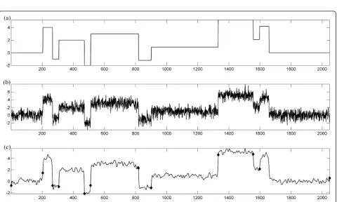
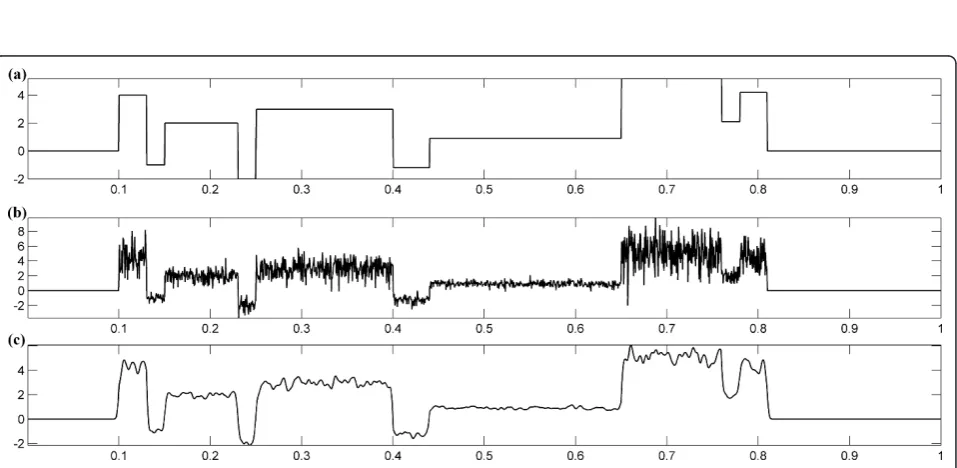
In this section, we will present the analysis of SSplit method in terms of MSE on four different types of syn-thetic signals [13]. MSE were computed between restored signal and original (noise free) signal. Figure 8 shows the restored Blocks signal with the proposed SSplit method along with the noisy block signal cor-rupted with white Gaussian noise. It can be seen from the figure that, the method not only reduced the noise significantly but also preserved the sharp transitions, which however is not in the case of mostly denoising algorithms. In the case of Block signal, the main prop-erty of such function lies in the discontinuity at the edges which has been preserved with the splitting.

Figure 9 shows the result on bumps signal corrupted with white Gaussian noise. In this case as well, the restored signal preserved the peaks along with the reduction of noise elements. The marked points in Fig-ure 9c represents the proposed split points. It can be seen from the figure that all the split points correspond to the peaks and once these peaks are identified, the restoration method result in smoothing rest of the noise elements. In the case of bumps signal, the selection of wM or wS is of extreme importance to get the best results as explained with an example of peak signal in the previous section.

(8)

Figure 7Explanation of wSandwMfactor.(a)Original and noisy signal: dotted line = original signal, solid line = noisy signal,(b) reconstruction withwS= 0.01, dotted line = original signal, solid line = reconstructed signal and root mean square error (RMSE) = 1.42,(c) reconstruction withwS= 0 and RMSE = 0.81, d) Reconstruction withwS= 0.007, dotted line = original signal, solid line = Reconstructed signal and RMSE = 0.32. RMSE were computed between restored signal and original (noise free) signal.

Figure 8Obtained results on Block signal.(a)Original block signal,(b)block signal with the addition of white Gaussian noise, sample size is 2048, input SNR (dB) is 9.25 and input MSE = 0.85,(c)reconstructed signal with SSplit (wS= 0.01), MSE = 0.36, (_Ψ(t)) is the first derivative of Gaussian function, the arrow marked shows the split point in the signal.

(9)

Figure 9Obtained results on Bumps signal.(a)Original bumps signal,(b)bumps signal with the addition of white Gaussian noise, sample size is 2048, input SNR (dB) is 10.16 and input MSE = 0.42, c) Reconstructed signal with SSplit (wS= 0.007), MSE = 0.23, (Ψ(t)) is the second derivative of Gaussian function, the arrow marked shows the split point in the signal.

(10)

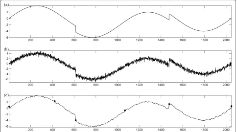
the case of Dopplers signal, the method split the signal from the points which correspond to the change in fre-quency. In many situations it is difficult to denoise low and high frequency components at the same time. How-ever, this can be done by splitting the signal. Similar results can be observed in the case of Heavisine signal as well. Apart from the smooth area, the proposed method preserved the sharp edges by splitting the signal from the discontinuities. In this section, we have pre-sented the results obtained with the SSplit method on four different types of signals used in this study. We will present the comparative analysis of the proposed method with the SURE shrinkage method in the follow-ing section.

The result on four different types of signals has been presented in this section. The main objective of the pre-sent study is to preserve these edges and then remove noise elements. Therefore, we first separate the sharp transition or edges from the signal by splitting and then performed smoothing operation. It can be seen from the results of block and heavisine signals that splitting pre-serve the main edges. After that we are left with the relatively homogeneous regions and we know that we need to perform smoothing along the data samples. However, this is not in the case of bumps signal because the only smoothing will result in generating an offset as

explained with an example in Section 4.2. Therefore, we try to find the better compromise between data samples and smoothness. Apparently, it seems to be a random selection but in fact, this is not the case. It can be seen from the results that the selection of the parametric value (wS) depends on the type of the signal.

5.1 Comparative analysis

Figure 12 shows the restored bumps signal with SURE shrink and the proposed SSplit method along with the noisy bumps signal corrupted with the white Gaussian noise. It can be seen from the figure that the restored signals from both approaches seem similar with a few differences in the mean square errors. In this study, all MSE were computed between reconstructed signal and original (noise free) signal. In the case of the bumps sig-nal, the most useful aspect and energy of the signal lies in the sharp peaks which shows the most significant transitions in the signal. Although the SURE Shrink method gives comparable results as compared to the SSplit method, but the energy of the peaks were reduced, as highlighted in Figure 12. The SSplit method preserves the energy of the peaks because the method split the signal from sharp peaks and restores the signal between such sharp transitions by considering regular points as explained in the previous section.

Figure 11Obtained results on Heavisine signal.(a)Original heavisine signal,(b)Heavisine signal with the addition of white Gaussian noise, sample size is 2048, input SNR (dB) is 16.85 and input MSE = 0.44,(c)reconstructed signal with SSplit (ws= 0.009), MSE = 0.13, (Ψ(t)) is the first derivative of Gaussian function, the arrow marked shows the split point in the signal.

(11)

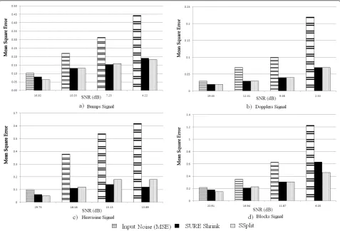
At the second stage, the method was tested with the addition of different variance of noise. The graphical results given in Figure 13 illustrate the resulting mean square error of four different types of signals with differ-ent variance of noise. It can be seen from the figure that the proposed method gives comparable results in all the cases with the classical SURE shrink method. Therefore, the method is particularly useful in the cases where the sharpness of the transitions is of extreme importance.

At the last stage, the proposed method has been com-pared with the SURE shrink approach with different size of data samples. Figure 14 summarizes the results in terms of MSE. It can be observed from the graphs that reduction in the total data samples does not significantly influence the results. The proposed method preserves the significant transition first and then performs smoothing and data sample based restoration. There-fore, after splitting, the subset or sub signal is left with the small transitions and relatively smoother regions, hence in most of the cases the reduction in the data sample does not significantly effect the denoising results. 5.1.1 Test with the multiplicative noise

The proposed method has been tested with an addition of multiplicative noise as well. In the case of multiplica-tive noise, variance of the noise is a function of the sig-nal and the noise variance is higher when amplitude of

the signal is higher. Figure 15 illustrates the amount of the multiplicative in the data samples and the effects of the denoising with the SSplit method. The proposed method works equally well in the case of multiplicative noise as well with the resulting root mean square error of 0.34. However, SURE shrink method needs some adaptation to perform in the presence of multiplicative noise.

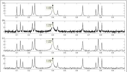
5.2 Generalization: extraction of small singularities The initial denoising results are very encouraging to extend this approach for the identification of small sin-gularities hidden inside the noisy signals. In contrast to the several proposed algorithms in the past, the SSplit method can detect small discontinuities or singularities hidden inside the signal. In several denoising methods, such small singularities are either suppressed during the denoising process or ignored due to their insignificance in most of the cases. These small but sharp singularities suffer due to the mutual influence of their adjacent high energy transitions [20], e.g., Figure 16 explains this phe-nomenon, where small edges are suppressed due to the mutual influence of its adjacent sharp transition. In Fig-ure 16, “A” defines the strength in terms of an ampli-tude of the strong discontinuity, whose influence does not allow the detection of adjacent small edge of an Figure 12Comparison: bumps signal.(a)Original bumps signal,(b)bumps signal with the addition of white Gaussian, sample size is 2048, input MSE = 0.3,(c)reconstruction with SURE Shrink method MSE = 0.16,(d)reconstructed signal with SSplit (ws_{= 0.007), MSE = 0.14, (}_Ψ₍_t_{)) is}

(12)

amplitude “1-A”. Since, splitting is based on the SURE based threshold criterion therefore, the selection of the correct thresholding scale is crucial to the accurate split-ting. Figure 16 shows the decay probabilistic curve of the SURE based threshold across successive scales along with the deterministic curve of small edge at“x” posi-tion (shown in Figure 16) with different A values. For each A value, edge at “x” can only be detected at the scale where the deterministic value is higher than the probabilistic value as Figure 17 highlights the minimum scale required to identify the edge at position“x”with a particular A value.

In order to identify such small edges, the SSplit method was extended to the multi splitting approach. It is possible to further split the subset by applying same splitting technique on subsets. Figure 18 gives the expla-nation of the multi splitting approach. At the first stage of splitting, the small discontinuity hidden at the loca-tion of “x” can not be detected. Therefore, the SSplit method is again applied on subset “C” to identify the small edge. Subset “C” is further split into two more subsets by using the same SSplit approach and finally

the complete denoised signal can be reconstructed by using total of 4 subsets. Figure 19 presents the results obtained with the multi SSplit method in the case of a small discontinuity (A = 0.8). It can be seen from the figure that the proposed method not only denoised the signal reasonably well but also preserved the small edges. On the other hand, SURE shrinkage method failed to do so.

5.3 Application: electrocardiogram signal

At the second stage, the proposed method has been applied on real signals. Electrocardiograms signal are used as test measure for this task. We applied SSplit method to denoised real Electrocardiogram signal. The detail theory of the method is already explained in the previous sections. Therefore very brief explana-tion of the implementaexplana-tion is given in this secexplana-tion. As already discussed before, the method is divided into two steps:

1. Signal Splitting.

2. Reconstruction or Restoration.

Figure 13Comparison of SURE shrink with SSplit method with different variance of input noise, sample size is 2048:(a)bumps,(b) dopplers,(c)heavisine,(d)blocks. Horizontal lines shows the MSE of input signal, solid black lines for SURE shrink and vertical lines for the resulting MSE with SSplit method. MSE computed between restored signal and original noiseless signals.

(13)

Figure 14MSE estimation comparison of SURE shrink with SSplit method with different sample size between 1024 and 8192:(a) bumps,(b)dopplers,(c)heavisine,(d)blocks. Horizontal lines shows the MSE of input signal, solid black lines for SURE shrink and vertical lines for the resulting MSE with SSplit method. MSE computed between restored signal and original noiseless signals.

Figure 15Comparison: blocks signal.(a)Original block signal,(b)block signal with an addition of multiplicative noise speckle noise, sample size is 2048, input MSE = 0.87,(c)reconstructed signal with SSplit (ws_{= 0.01), MSE = 0.34, (}

(14)

5.3.1 Electrocardiogram signal splitting

In order to split the signal multiscale analysis has been applied on ECG signal. 2ndorder Gaussian wavelet func-tion has been used as an analyzing wavelet funcfunc-tion for decomposition into succesive scales. The main reason for the selection of Gaussian wavelet function is its

close similarity with the ECG signal and to ensure the evolution of modulus maxima on each scale as explained already in previous chapter. The CWT and the CWT based modulus maxima are two good tools for the analysis of ECG and both exhibit good perfor-mance even in the presence of noise. The low level of Figure 16Multisplitting.(a)Synthetic block function with two discontinuities,_“A_”represents the strength in terms of an amplitude of the high step and(b)function with the white Gaussian noise (0,1).

Figure 17Evolution of maxima at position“x“by varying A amplitude, along with the probabilistic SURE threshold curve (dashed line). For each A value, edge at position“x“can only be detected at the scale where the deterministic value is higher than the probabilistic value.

(15)

computational complexity of the modulus maxima makes it easier of the two to employ in practice. How-ever, for the detection of small waveform features within the ECG, the CWT contains more detailed information and therefore has the potential to produce enhanced results.

In order to illustrate the performance of the SSplit method on real signal, the real ECG signal taken from MIT-BIH website [21] has been taken (shown in

(16)

subsets. It can be seen from the modulus maxima cor-respond to the coarsest scale of the multiscale analysis that the thresholding will result in giving only the R peaks point as the split points and after the threshold-ing this assumption was justified. The signal has been split from the corresponding R peaks and hence the reconstruction process was applied between these peaks.

5.3.2 Electrocardiogram signal restoration

Figure 23a shows the marked points as proposed split points. It can be concluded that all the peaks points are considered to be as a split points and the reconstruction

was performed between all these peaks. Unlike pre-viously proposed denoising method, the main signifi-cance of the present approach is the preservation of energy in the peaks. Figure 22 presents the modulus maxima lines of the corresponding ECG signal. It has been explained before that these lines correspond to all the modulus maxima on successive scales and the local regularity can be measured from these line by Lipschitz exponents. We had identified all the regular points from this measure and then applied the restoration process as already explained in detail in previous section. Since, we already defined in previous chapter that weighing factors Figure 19Results with multisplitting.(a)Original signal,(b)noisy signal input RMSE (0.20),(c)SURE shrink results RMSE = 0.092,(d)SSplit with extended multi splitting approach (A = 0.8), RMSE = 0.032.

Figure 20Real electrocardiogram signal taken from MIT-BIH website (MIT 100.dat). Jalilet al.EURASIP Journal on Advances in Signal Processing2012,2012:38

http://asp.eurasipjournals.com/content/2012/1/38

(17)

wS orwMare manual inputs and depends on the nature of the signal. But for the given ECG signals, the weigh-ing factorswSor wMare kept same as in Bumps signals

(wS = 0.007) and the main reason for this selection is the close approximation of both signals. Figure 23 pre-sents the denoising results. In order to illustrate the Figure 21Multiscale analysis of electrocardiogram signal.

(18)

performance of the method, we have added known white Gaussian noise (10dB). It can be seen from the figure that the new method has successfully reduce the noise elements without introducing any spurious oscilla-tions with the resulting MSE = 0.21. Not only that, it can be observed that the energy inside the peaks has also been preserved. The method has been tested with different types of signal given in the database and in term of statistics, the resulting MSE of almost 83% of the different cases of ECG is less than 0.23.

5.4 Discussions

Although in the present form, the method performed very well on signals where small information about the nature of the signals are apriori known, e.g., if it is elec-trocardiogram (ECG) signal, speech signal or mechanical vibrations. With this information, it is possible to roughly estimate the parametric value ofwS. This is due to the fact that if system is design for the denoising of ECG signal then all the ECG signals have approximately similar structure, same goes for the other types of the signals. In this context, we say that the proposed method is semi automatic in nature. With a very little information, the method effectively denoise any type of the signal in the case of either additive or multiplicative noise elements. In addition to that, If we know that the smoothness is of high priority then we can assign higher

weighage to wS. It has already been explained in the Section 4.2, that the maximum smoothness gives visually best results with the splitting but higher statistical error in term of MSE.

At the current stage, we are working on the possible solutions to completely automate the method. One approach could be to relate the smoothness of the signal with the type of singularities present inside the signal (shown in Figure 5). However, further experiments are needed to relate the type of singularity (Lipschitz value) with the choice ofwSand will be presented in the future study.

6 Conclusion

In the present study, a novel approach for the restora-tion of signals from noisy data samples has been pre-sented. The most useful aspect of the proposed method is the separation of sharp edges or transitions from the suspicious noise elements. Based on the SURE estima-tion, thresholding is performed on modulus maxima across selected scales to split the signal from the edges. The wavelet transform has shown to be a useful tool to extract noise elements by locating modulus maxima. Lipschitz exponents computed from modulus maxima lines can be used to identify the noise elements. The reconstruction process involves in finding the best com-promise between the data samples in terms of MSE and Figure 23Implementation on real signals.(a)Original ECG signal,(b)ECG signal with white Gaussian noise.(c)Denoising with SSplit method (marked points are proposed split points).

(19)

the smoothing criteria. The trade off between mean square error and the smoothing criteria can be opti-mized and it depends on the type of singularity present inside the signal. It has been shown with an example (peak signal in Figure 6) that it is possible to have bad results in terms of MSE even though the results visually appears to be good in terms of smoothness. Moreover due to the detection of singularities, an over smoothing will not really change the shape of the signal and main information about the shape of the signal has been pre-served. Graphical results shown in the figures demon-strate that the proposed method performs equally well as compared to the conventional shrinkage methods at different variance of noise and sample sizes. The present method is particularly useful for the extraction of small singularities hidden inside the signal. Perspective will be focus on such small edges which cannot be detected due to the mutual influence of their adjacent strong transitions. However, splitting the signal into significant subsets allows such small hidden singularities to be identified. Furthermore, the proposed method proved that the denoising in spatial domain work equally well as in transform domains. By looking at the statistical and graphical results, it could be quite logical to extend the method for 2D cases. We will present the extension of this method in 2D cases and our findings in future study.

Appendix

In this section, once again we are summarizing the method as follows:

1. At the first step, the signal has been divided into different subsets or sub signal. The selection of these subsets is defined on the basis of SURE based nonlinear thresholding of WTMM.

2. The second step is to identify Lipschitz exponents computed from each subsets individually. These Lipschitz exponent results in identifying the regular points present in the subset. In the present study, all the differentiable points (a ≥1) are considered as regular points.

3. The nonlinear function is then optimized between all regular points to restore each subset individually by following reconstruction algorithm as follows:

Step1 : Initialization k= 1,Y_i1=Y_oi1

Step 2 :

Y_ik+1=Y_ik+wMλk_i

−∂C

MSE,k i ∂Yi

+wSγ_ik

−∂C

MSO,k i ∂Yi

Step3 : if_N1N− 1

l=0

yk_i_,_l−yk_i_,+1_l 2< ε

Stop else k=k+ 1

εis the minimum root mean square error and lis the index of data sample.

Competing interests

The authors would like to acknowledge Region Bourgogne, France for providing financial support, Dr. Zegadi, Dr. Nasera Zegadi, Dr. Aneza, Dr. Azeem, Dr. El Habbach and Dr. Soussou for their valuable help in understanding the different concepts of electrocardiogram signals. We are also thankful of Florian Luisier for his kind help in understanding SURE-LET denoising method.

Received: 2 May 2011 Accepted: 20 February 2012 Published: 20 February 2012

References

1. A Antoniadis, J Bigot, T Sapatinas, Wavelet estimators in nonparametric regression: a comparative simulation study. J Statist Softw.6, 1_–83 (2001) 2. S Mallat,A Wavelet Tour of Signal Processing, 2nd edn. (Academic Press,

New York, 1999)

3. S Mallat, W Huwag, Singularity detection and processing with Wavelets. IEEE Trans Inf Theory.38, 617–643 (1992). doi:10.1109/18.119727 4. A Liew, DT Nguyen, Reconstruction from wavelet transform modulus

maxima using non-expansive projections. Electron Lett.31, 1038–1039 (1995). doi:10.1049/el:19950749

5. Z Cvetkovic, M Vetterli, Wavelet extrema and zero-crossing representation: Properties and consistent reconstruction, inIEEE International Conference on Acoustics Speech and Signal Processing.3, III/117–III/120 (1994)

6. CJ Kicey, CJ Lennard, Unique reconstruction of band-limited signals by a Mallat-Zhong Waveletbbtransform algorithm. J Fourier Anal Appl.3, 63–82 (1997). doi:10.1007/BF02647947

7. B Jalil, O Beya, E Fauvet, O Laligant, Detection of QRS complex in ECG signal based on classification approach, inInternational Conference on Image Processing (ICIP), Hong Kong, pp. 345–348 (2010)

8. V Brunia, D Vitulano, Wavelet-based signal de-noising via simple singularities approximation. Signal Process.86, 859_–876 (2006). doi:10.1016/j. sigpro.2005.06.017

9. TC Hsung, DP Lun, WC Siu, Denoising by singularity Detection. IEEE Trans Signal Process.47, 3139–3144 (1999). doi:10.1109/78.796450

10. C Ordenovica, C Suracea, B Torresani, A Llebaria, Detection of glitches and signal reconstruction using Holder and wavelet analysis. Statist Methodol.5, 373–386 (2008). doi:10.1016/j.stamet.2008.01.005

11. F Jin, P Fieguth, L Winger, Wavelet video denoising with regularized multiresolution motion estimation. EURASIP J Appl Signal Process.2006, 1_–11 (2006)

12. GY Chen, TD Bui, Multiwavelets denoising using neighboring coefficients. IEEE Signal Process Lett.10, 211_–214 (2003)

13. DL Donoho, I Johnstone, Ideal spatial adaptation via wavelet shrinkage. Biometrika.81, 425_–455 (1994). doi:10.1093/biomet/81.3.425

14. RR Coifman, DL Donoho, Translation-invariant Denoising, inLecture Notes in Statistics, (Springer Verlag, New York, 1995)

15. L Xiao, LL Huang, B Roysam, Image variational denoising using gradient fidelity on curvelet shrinkage. EURASIP J Adv Signal Process.2010, 1–16 (2010) 16. AM Atto, D Pastor, G Mercier, Smooth adaptation by sigmoid shrinkage.

EURASIP J Image Video Process,2009, Article ID 532312.16(2009). 17. IK Fodor, C Kamath, Denoising through wavelet shrinkage: an empirical

study. J Electron Imag.12, 151–160 (2003). doi:10.1117/1.1525793 18. T Blu, F Luisier, The SURE-LET approach to image denoising. IEEE Trans

Image Process.16, 2778–2786 (2007)

19. S Charles, Estimation of the mean of a multivariate normal distribution. Annals Statist.9, 1135–1151 (1981). doi:10.1214/aos/1176345632

20. O Laligant, F Truchetet, F Meriaudeau, Regularization preserving localization of close edges. IEEE Signal Process Lett.14, 185–188 (2007)

21. MIT-BIH Arrhythmia Database http://www.physionet.org/physiobank/ database/mitdb

doi:10.1186/1687-6180-2012-38

Cite this article as:Jalilet al.:Signal restoration via a splitting approach.