A comparison of nonlinear filtering approaches in the context of an HIV model

(1)

A Comparison of Nonlinear Filtering

Approaches in the Context of an HIV Model

H.T. Banks, Shuhua Hu, Zackary R. Kenz and H.T. Tran

Center for Research in Scientiﬁc Computation North Carolina State University

Raleigh, NC 27695-8212

July 16, 2009

Abstract

In this paper three different filtering methods, the Extended Kalman Filter (EKF), the Gauss-Hermite Filter (GHF), and the Unscented Kalman Filter (UKF), are com-pared for state-only and coupled state and parameter estimation when used with log state variables of a model of the immunologic response to the human immunodeficiency virus (HIV) in individuals. The filters are implemented to estimate model states as well as model parameters from simulated noisy data, and are compared in terms of estimation accuracy and computational time. Numerical experiments reveal that the GHF is the most computationally expensive algorithm, while the EKF and UKF have comparable computation times. In addition, computational experiments suggest that there is little difference in the estimation accuracy between the UKF and GHF. When measurements are taken as frequently as every week to two weeks, the EKF is the superior filter. When measurements are further apart, the UKF is the best choice in the problem under investigation.

1 Introduction

The modeling of the physiologic and immunologic response to HIV infection in humans is generating a substantial amount of research effort, and significant progress has been made in the treatment of HIV-infected patients. One of the most prevalent treatment strategies for acutely infected HIV patients is highly active anti-retroviral therapy (HAART) which utilizes two or more drugs. However, despite the success of HAART, patient-specific optimal schemes for its use need to be considered. Grave side effects of taking drugs, viral mutations and the high cost of drugs all motivate a substantial research effort in this area.

(2)

reasons such as poor patient adherence, increasing drug resistance due to virus mutations, and drug side eﬀects as noted. Another approach that has been used to design dynamic HIV treatment therapies utilizes feedback controls such as those based on the state dependent Riccati equation (SDRE) approach used in [6] and on receding horizon control methodology in [8]. A fundamental characteristic of feedback control is that it depends on the current

state of the system. Hence, this method can be used to designadaptive treatment schedules

for HIV patients based on the patient’s current status (e.g., current CD4+ T cell count and viral load). Because HIV modeling generally involves partial observations and noisy measurements from combined compartments, the method by which the state is obtained at each sampling time is of special concern, and an eﬃcient estimation technique is needed to develop a successful implementation of feedback control.

State and parameter estimation and the development of associated adaptive feedback control schemes in the setting investigated here offer challenges different from those in many engi-neering applications where often high frequency uncensored observations are often the norm. In addition to low frequency sampling in longitudinal data sets (data points are often very expensive both in financial costs of associated assays as well as in emotional/physical costs to patients), the data itself is frequently censored below due to limitations on assays in dis-criminating low values. Thus a number of challenges include development of filters for state and parameter estimation in the context of low frequency sampling and partial state obser-vations that are censored. Successful efforts in these areas must be combined with feedback control of nonlinear dynamics which are often only approximate for patient response. Here we discuss a first step in development of a needed methodology by attempting to discover an appropriate filtering approach to use with partial state uncensored observations that are collected rather infrequently by usual engineering standards.

The model used in this paper was developed and validated as a predictive tool in [4], wherein two types of target cells, along with their corresponding infected states, free virus, and im-mune eﬀector cells (CTL) are included as states in the model. Fitting with clinical data demonstrated that this model provides reasonable ﬁts to numerous patient longitudinal data sets and has impressive predictive capability when comparing model simulations with param-eters based on estimation using only half of the longitudinal observations. For computational

ease in our presentation here, without loss of generality, we omit the noninfectious virus𝑉𝑁 𝐼

component from the model in [4]. This will not aﬀect the dynamics of this model as it is completely decoupled from all the other compartments. The model we use is

˙

𝑇1 = 𝜆1−𝑑1𝑇1−(1−𝜖1)𝑘1𝑉𝐼𝑇1

˙

𝑇2 = 𝜆2−𝑑2𝑇2−(1−𝜇𝜖1)𝑘2𝑉𝐼𝑇2

˙

𝑇∗

1 = (1−𝜖1)𝑘1𝑉𝐼𝑇1−𝛿𝑇1∗−𝑚1𝐸𝑇1∗

˙

𝑇∗

2 = (1−𝜇𝜖1)𝑘2𝑉𝐼𝑇2−𝛿𝑇2∗−𝑚2𝐸𝑇2∗ (1)

˙

𝑉𝐼 = 𝑁𝑇103𝛿(𝑇1∗+𝑇2∗)−[𝑐+ (1−𝜖1)103𝑘1𝑇1+ (1−𝜇𝜖1)103𝑘2𝑇2]𝑉𝐼 ˙

𝐸 = 𝜆𝐸 +𝑏𝐸

𝑇∗

1 +𝑇2∗ 𝑇∗

1 +𝑇2∗+𝐾𝑏

𝐸−𝑑𝐸

𝑇∗

1 +𝑇2∗ 𝑇∗

1 +𝑇2∗+𝐾𝑑

(3)

with a state vector initial condition

(𝑇1(0), 𝑇2(0), 𝑇1∗(0), 𝑇2∗(0), 𝑉𝐼(0), 𝐸(0))𝑇.

Here the state variables are 𝑇1, the uninfected CD4+ T-cells; 𝑇2, the uninfected target cells

of a second kind; 𝑇∗

1, the infected CD4+ T-cells; 𝑇2∗, the infected target cells of a second

kind; 𝑉𝐼, the infectious virus; and 𝐸, the immune eﬀectors. The units for 𝑇1, 𝑇2, 𝑇1∗, 𝑇2∗

and 𝐸 are cells/𝜇l-blood, and the unit for 𝑉𝐼 is RNA copies/ml-plasma. The factors 103

are introduced to convert between microliter (𝜇l) and milliliter (ml) scales, preserving the

units from some of the earlier published papers [1]. The particular target cells of a second kind are not speciﬁed, and (according to [4]) might be related to macrophages or brain cells or inactivated memory. The model also includes terms that model drug eﬃcacy. The

control term𝜖1 represents the eﬃcacy of a Reverse Transcriptase Inhibitor (RTI). For a more

detailed description of model parameters and rationale for the model (1) we refer the reader to the article [4]. While there are somewhat improved and generalized versions of this model [5], the version we have chosen to use here is representative and more than adequate for demonstration of the behavior of the classes of ﬁlters we wish to compare.

We observe that our model (1) is nonlinear and hence we must explore nonlinear estimation methods. The Extended Kalman Filter (EKF) was used in [9] for state estimation for the

HIV model of [4] (also without the 𝑉𝑁 𝐼 component and without the scaling factor). Unlike

the nonlinear least squares approach this technique does not require all the data at once. That is, this methodology only uses data as it is received and thus it can be used “online” to estimate the parameters in an adaptive approach. However, the EKF was found in [9] to have difficulty with state estimation even when the time span between measurements is only five days. This motivates a need to consider alternative filtering methods. Accordingly, we introduce the Gauss-Hermite Filter (GHF) and Unscented Kalman Filter (UKF) as possible alternatives. Even though all three of theses methods are based on a Gaussian assumption (that is, the posterior distribution can be approximated by a Gaussian distribution), the process by which this approximation is obtained is different, and therefore, leads to different performance. It has been demonstrated (e.g., [10, 15]) that the performance of both the GHF and UKF are superior to the EKF in numerous other nonlinear problems.

Even though this paper might be considered an extension of the efforts in [9], we have made a significant modification here in applying these filters to our problem. Instead of using the

model directly as in [9], we applied the ﬁlters to a log-scaled version of our model. This

was done because log-transformation is a standard technique to render the observations more nearly normally distributed. In addition, from a numerical analysis point of view, by using a log-transformed system one can resolve a problem of states becoming unrealistically negative due to round-oﬀ errors. More importantly, all these ﬁlters are derived for systems

where the states are deﬁned onℝ𝑛; this may lead to some trouble when one apples the ﬁlters

to a system such as (1) where the states are only deﬁned in ℝ𝑛

+; log-scaling mitigates this

potential diﬃculty.

(4)

of the EKF, UKF and GHF and their application to a general nonlinear continuous system with discrete observations. In Section 3, the ﬁlters are implemented to estimate model states as well as model parameters from simulated noisy data, and compared in terms of estimation accuracy and computational time. We conclude the paper in Section 4 with some remarks and suggestions for future eﬀorts.

2 Filter Descriptions

In this section we will use a capital italic letter to denote a random variable or random vector unless otherwise indicated, and use the corresponding small letter to denote its realization. A capital Roman letter is used to denote a non-random matrix. In addition, we may

occa-sionally use the following shorthand notations to ease the presentation: 𝑋𝑡 for 𝑋(𝑡), 𝑃𝑡𝑡𝑘𝑘+1

for P𝑡𝑘₍_𝑡

𝑘+1), etc. We will useℰ{⋅}to denote the expectation of a random variable or vector.

Next we give a brief introduction of the three ﬁlters that we use, the EKF, GHF and UKF, and their application in the context of a general nonlinear continuous system

𝑑𝑋(𝑡) = 𝑓(𝑋(𝑡), 𝑡)𝑑𝑡+𝜎(𝑡)𝑑𝐵(𝑡), 𝑡 ≥𝑡0, (2)

with discrete observations taken according to the measurement equation

𝑌𝑘=ℎ(𝑋(𝑡𝑘), 𝑡𝑘) +𝑉𝑘, 𝑡𝑘+1 > 𝑡𝑘 ≥𝑡0, 𝑘= 1,2,3, . . . .

Here 𝑋(𝑡), assumed to satisfy an Ito stochastic diﬀerential equation, is a 𝑛-dimensional

column vector random variable for any ﬁxed time𝑡with𝑋𝑡0 being normally distributed with

mean ˆ𝑥𝑡0 and covariance matrix P𝑡0, i.e.,𝑋𝑡0 ∼ 𝒩(ˆ𝑥𝑡0,P𝑡0),𝑓 :ℝ

𝑛_×ℝ_→_ℝ𝑛_{is a non-random}

function of 𝑥 and 𝑡, 𝐵(𝑡) is 𝑟-dimensional Brownian motion with ℰ[(𝑑𝐵(𝑡))(𝑑𝐵(𝑡))𝑇_{] =}

Q(𝑡)𝑑𝑡, where Q(𝑡) is an𝑟×𝑟 matrix, and𝜎:ℝ→ℝ𝑛×𝑟 is a non-random function of time𝑡.

The random variable𝑌𝑘 is a𝑙-dimensional column vector, ℎ:ℝ𝑛×ℝ→ℝ𝑙 is a non-random

function of 𝑥and 𝑡, and𝑉𝑘 are white Gaussian random sequence with 𝑉𝑘 ∼ 𝒩(0,R𝑘), where

R𝑘 is a 𝑙×𝑙 matrix. In addition, we assume that𝑋𝑡0, {𝐵(𝑡)} and {𝑉𝑘} are independent.

Let𝒴𝜏 ={𝑦𝑘 :𝑡𝑘≤𝜏}denote the information available by observing the process up to time

𝜏, where𝑦𝑘 is a realization of𝑌𝑘. The ﬁltering problem is to ﬁnd the “best” estimate ˆ𝑥𝜏(𝑡)

of𝑋(𝑡) based on𝒴𝜏. The “best” is understood in the sense of minimum mean-squared error

(MMSE) for each ﬁxed 𝑡

ˆ

𝑥𝜏₍_𝑡_{) = arg min}

𝜉 ℰ

{

(𝑋(𝑡)−𝜉)𝑇₍_𝑋₍_𝑡₎₋_𝜉₎_∣𝒴

𝜏

} ,

where the superscript in ˆ𝑥𝜏 _{is determined by the subscript in}_𝒴

𝜏. The MMSE estimate ˆ𝑥𝜏(𝑡)

of 𝑋(𝑡) based on 𝒴𝜏 is the conditional mean

ˆ

(5)

and the covariance matrix of this estimate, denoted by P𝜏(𝑡), is given by P𝜏₍_𝑡_{) =}_ℰ{₍_𝑋₍_𝑡₎₋_𝑥_ˆ𝜏₍_𝑡₎₎₍_𝑋₍_𝑡₎₋_𝑥_ˆ𝜏₍_𝑡₎₎𝑇_∣𝒴

𝜏}.

Hence, to determine the best estimate ˆ𝑥𝜏(𝑡) of 𝑋(𝑡) based on 𝒴𝜏 as well as the conditional

covariance matrix, we need to ﬁnd the conditional probability density function 𝑝(𝑥, 𝑡∣𝒴𝜏) of

𝑋(𝑡) at any time 𝑡. However, this distribution 𝑝(𝑥, 𝑡∣𝒴𝜏), which satisﬁes the Fokker-Planck

equation between any observation period 𝑡𝑘 < 𝑡 < 𝑡𝑘+1,

∂𝑝(𝑥, 𝑡∣𝒴𝜏)

∂𝑡 +

𝑛

∑

𝑖=1

∂(𝑝(𝑥, 𝑡∣𝒴𝜏)𝑓𝑖(𝑥, 𝑡))

∂𝑥𝑖

= 1

2 𝑛

∑

𝑖=1

𝑛

∑

𝑗=1

∂2_[(_𝜎₍_𝑡_)Q(_𝑡₎_𝜎𝑇₍_𝑡₎₎

𝑖𝑗𝑝(𝑥, 𝑡∣𝒴𝜏)]

∂𝑥𝑖∂𝑥𝑗

,

and then is updated with a measurement due to a new observation at 𝑡𝑘+1 using Bayes

formula, in general, can not be obtained in closed form. Hence, in many applications it is conventionally assumed that the distribution is Gaussian so that the distribution is com-pletely parameterized by just the mean and covariance; this is exactly the assumption made in the EKF, GHF and UKF.

All three ﬁlters, the EKF, UKF and GHF, utilize a “predictor-corrector” implementation.

Given current state estimate ˆ𝑥𝑡𝑘

𝑡𝑘 = ˆ𝑥

𝑡𝑘₍_𝑡

𝑘) and covariance matrix estimate P𝑡𝑡𝑘𝑘 = P

𝑡𝑘₍_𝑡

𝑘)

at time 𝑡𝑘, the ﬁlter ﬁrst predicts the states at time𝑡𝑘+1 by using only model dynamics to

obtain the predicted quantities ˆ𝑥𝑡𝑘

𝑡𝑘+1 = ˆ𝑥

𝑡𝑘(𝑡

𝑘+1) and P𝑡𝑡𝑘𝑘+1 = P

𝑡𝑘(𝑡

𝑘+1). When new data𝑦𝑘+1

is available at time 𝑡𝑘+1, a linear update rule is speciﬁed to obtain the updated quantities

ˆ

𝑥𝑡𝑘+1

𝑡𝑘+1 and P

𝑡𝑘+1

𝑡𝑘+1, where the weights are chosen to minimize the mean squared error of the

estimate.

2.1 The Extended Kalman Filter

In the EKF, the expected values occurring in time and measurement updates are computed

by linearization of the system function 𝑓 and measurement function ℎ at the current state

estimate.

To start the ﬁlter algorithm, we set 𝑘 = 0 initially and set ˆ𝑥𝑡0

𝑡0 = ˆ𝑥𝑡0 and P

𝑡0

𝑡0 = P𝑡0 for given

initial conditions ˆ𝑥𝑡0, P𝑡0. We then compute the predicted state ˆ𝑥

𝑡𝑘

𝑡𝑘+1 = ˆ𝑥

𝑡𝑘₍_𝑡

𝑘+1), by solving

the ordinary diﬀerential equations

𝑑𝑥ˆ𝑡𝑘(𝑡)

𝑑𝑡 =𝑓(ˆ𝑥

𝑡𝑘(𝑡), 𝑡), 𝑡

𝑘 < 𝑡 < 𝑡𝑘+1,

ˆ

𝑥𝑡𝑘₍_𝑡

𝑘) = ˆ𝑥𝑡𝑡𝑘𝑘.

We simultaneously compute the predicted error covariance matrix P𝑡𝑘

𝑡𝑘+1 = P

𝑡𝑘(𝑡

𝑘+1), by

solving the ordinary diﬀerential equations

𝑑P𝑡𝑘(𝑡)

𝑑𝑡 = P

𝑡𝑘₍_𝑡₎[_▽_𝑓_(ˆ_𝑥𝑡𝑘₍_𝑡₎_{, 𝑡}₎]𝑇 ₊_▽_𝑓_(ˆ_𝑥𝑡𝑘₍_𝑡₎_{, 𝑡}_)P𝑡𝑘₍_𝑡_{) +}_𝜎₍_𝑡_)Q(_𝑡₎_𝜎𝑇₍_𝑡₎_, _𝑡

𝑘< 𝑡 < 𝑡𝑘+1,

(6)

Here 𝑄 and 𝜎 are the parameters of the noise in the stochastic process 𝑋(𝑡) as described above. Once this prediction step is complete, we can incorporate the new data information

at time 𝑡𝑘+1. We compute the updated state and updated error covariance matrix with the

observation 𝑦𝑘+1 by computing solutions to the equations

ˆ

𝑥𝑡𝑘+1

𝑡𝑘+1 = ˆ𝑥

𝑡𝑘

𝑡𝑘+1 + G𝑘+1(𝑦𝑘+1−ℎ(ˆ𝑥

𝑡𝑘

𝑡𝑘+1, 𝑡𝑘+1)),

and

P𝑡𝑘+1

𝑡𝑘+1 =

[

I−G𝑘+1▽ℎ(ˆ𝑥𝑡𝑡𝑘𝑘+1, 𝑡𝑘+1) ]

P𝑡𝑘

𝑡𝑘+1,

respectively, where G𝑘+1 is deﬁned by

G𝑘+1 = P𝑡𝑡𝑘𝑘+1 (

▽ℎ(ˆ𝑥𝑡𝑘

𝑡𝑘+1, 𝑡𝑘+1)

)_𝑇 [

𝑡𝑘+1, 𝑡𝑘+1)P

𝑡𝑘

𝑡𝑘+1

(

𝑡𝑘+1, 𝑡𝑘+1)

)_𝑇

+ R𝑘+1

]₋₁ .

Recall that R𝑘 is the covariance matrix in the noise for the observation process. We thus

have the updated state values and covariance matrix at time𝑡𝑘+1. We then move to the next

time step, so we increment 𝑘 by 1 and return to the predictor step.

The EKF has been successfully applied to numerous nonlinear ﬁltering problems in the engineering and physical sciences. However, its performance can be extremely poor when nonlinearities between observations become severe. Moreover, it is not a good choice for some application problems where Jacobian matrices are diﬃcult to calculate (or may not even exist). For more discussions on the EKF, the interested reader can consult [11] among numerous other texts.

2.2 The Unscented Kalman Filter

Instead of linearization of the system function𝑓 and measurement functionℎat current state

estimates as required by the EKF, in order to compute the expected values occurring in time and measurement updates, the UKF is based on the principle that a discrete distribution composed of a set of deterministically chosen sampled points with the corresponding weights can be used to approximate the standard normal distribution. It is founded on intuition: “it is easier to approximate a probability density function than it is to approximate an arbitrary

nonlinear function”. Given a function ˜𝑓(𝜏), the UKF entails the approximation of integrals

by

∫

ℝ𝑛

˜

𝑓(𝜏) 1 (2𝜋)𝑛/2𝑒

−1

2∣𝜏∣2𝑑𝜏 ≈

𝑁

∑

𝑖=1

˜

𝑓(𝑞𝑖)𝑤𝑖. (3)

Here𝑁 = 2𝑛+ 1. The values for the sampling points 𝑞𝑖 and the weights𝑤𝑖 are deﬁned by

𝑞𝑖 =

⎧ ⎨

⎩

√

𝑛+𝜅𝑒𝑖, 1≤𝑖≤𝑛,

−𝑞𝑖−𝑛, 𝑛+ 1≤𝑖≤2𝑛,

0, 𝑖= 2𝑛+ 1,

and 𝑤𝑖 =

⎧   ⎨

  ⎩

1

2(𝑛+𝜅), 1≤𝑖≤2𝑛,

2𝜅

(7)

where 𝑒𝑖 is the 𝑖th unit vector in ℝ𝑛, and 𝜅 ∈ ℝ can be any number providing 𝑛+𝜅 ∕= 0.

The variable𝜅provides an extra degree of freedom to “ﬁne tune” the higher order moments

of the approximation and can be used to reduce the overall predication error.

The UKF was originally designed for a discrete system with discrete observations. To apply

to the continuous model (2) we need to discretize the model over each time frame (𝑡𝑘, 𝑡𝑘+1).

We ﬁrst subdivide the interval (𝑡𝑘, 𝑡𝑘+1) into the 𝑀 subintervals (𝑡𝑘 + (𝑗 −1)𝛿𝑡, 𝑡𝑘 +𝑗𝛿𝑡)

where 1≤𝑗 ≤𝑀 and 𝛿𝑡 = (𝑡𝑘+1−𝑡𝑘)/𝑀. Then we use an Euler method approximation

𝑋𝑘,𝑗 ₌_𝑋𝑘,𝑗−1₊_𝛿

𝑡𝑓(𝑋𝑘,𝑗−1, 𝑡𝑘+ (𝑗−1)𝛿𝑡) +𝜎(𝑡𝑘+ (𝑗 −1)𝛿𝑡)𝑊𝑘,𝑗, 1≤𝑗 ≤𝑀 (4)

with 𝑊𝑘,𝑗 =𝐵(𝑡𝑘+𝑗𝛿𝑡)−𝐵(𝑡𝑘+ (𝑗−1)𝛿𝑡), where𝑋𝑘,𝑗 denotes the ﬁnite diﬀerence

approx-imation of𝑋(𝑡𝑘+𝑗𝛿𝑡).

To begin the ﬁlter algorithm, we set𝑘 = 0 and set ˆ𝑥𝑡0

𝑡0 = ˆ𝑥𝑡0 and P

𝑡0

𝑡0 = P𝑡0. We then compute

the predicted state ˆ𝑥𝑡𝑘

𝑡𝑘+1 = ˆ𝑥

𝑡𝑘₍_𝑡

𝑘+1), and the predicted covariance matrix P𝑡𝑡𝑘𝑘+1 = P

𝑡𝑘₍_𝑡

𝑘+1)

through the time frame 𝑡𝑘 < 𝑡 < 𝑡𝑘+1. To begin the predictor step, we set 𝑗 = 0, pick

𝑀 >0, and let 𝛿𝑡 = (𝑡𝑘+1−𝑡𝑘)/𝑀. Then compute the factorization P𝑡_𝑡𝑘_𝑘₊₍_𝑗₋₁₎_𝛿_𝑡 = S𝑇S using

the Cholesky decomposition. Set ˜𝑥𝑖 = S𝑇𝑞𝑖 + ˆ𝑥_𝑡𝑡𝑘_𝑘₊₍_𝑗₋₁₎_𝛿_𝑡. We then compute the following

sums to obtain the states and the covariance matrix

ˆ

𝑥𝑡𝑘

𝑡𝑘+𝑗𝛿𝑡 =

𝑁

∑

𝑖=1

(˜𝑥𝑖+𝛿𝑡𝑓(˜𝑥𝑖, 𝑡𝑘+ (𝑗 −1)𝛿𝑡))𝑤𝑖,

P𝑡𝑘

𝑡𝑘+𝑗𝛿𝑡 =

𝑁

∑

𝑖=1

(˜𝑥𝑖+𝛿𝑡𝑓(˜𝑥𝑖, 𝑡𝑘+ (𝑗 −1)𝛿𝑡)−𝑥ˆ𝑡𝑡𝑘𝑘+𝑗𝛿𝑡)(˜𝑥𝑖+𝛿𝑡𝑓(˜𝑥𝑖, 𝑡𝑘+ (𝑗−1)𝛿𝑡)−𝑥ˆ

𝑡𝑘

𝑡𝑘+𝑗𝛿𝑡)

𝑇_𝑤

𝑖

+𝜎(𝑡𝑘+ (𝑗−1)𝛿𝑡)Q(𝑡𝑘+ (𝑗 −1)𝛿𝑡)𝜎(𝑡𝑘+ (𝑗−1)𝛿𝑡)𝑇.

After the sums have been computed, we increment𝑗and repeat the preceding steps beginning

with the factorization of P𝑡𝑘

𝑡𝑘+(𝑗−1)𝛿𝑡. We continue iterating until𝑗 =𝑀, which will yield ˆ𝑥

𝑡𝑘

𝑡𝑘+1

and P𝑡𝑘

𝑡𝑘+1.

Once this prediction step is complete, we can incorporate the new data information at

time 𝑡𝑘+1 to update the state and covariance matrix. First, we compute the factorization

P𝑡𝑘

𝑡𝑘+1 = ˜S

𝑇_{˜S as before and set ˜}_𝑥

𝑖 = ˜S𝑇𝑞𝑖+ ˆ𝑥𝑡𝑡𝑘𝑘+1. Then compute

ˆ

𝑥𝑡𝑘+1

𝑡𝑘+1 = ˆ𝑥

𝑡𝑘

𝑡𝑘+1 + L𝑘+1(𝑦𝑘+1−𝑧𝑘+1),

P𝑡𝑘+1

𝑡𝑘+1 = P

𝑡𝑘

𝑡𝑘+1−L𝑘+1P

𝑇

(8)

where

𝑧𝑘+1 =

𝑁

∑

𝑖=1

ℎ(˜𝑥𝑖, 𝑡𝑘+1)𝑤𝑖,

P𝑥𝑧 =

𝑁

∑

𝑖=1

(˜𝑥𝑖−𝑥ˆ𝑡𝑡𝑘𝑘+1)(ℎ(˜𝑥𝑖, 𝑡𝑘+1)−𝑧𝑘+1)

𝑇_𝑤

𝑖,

P𝑧𝑧 =

𝑁

∑

𝑖=1

(ℎ(˜𝑥𝑖, 𝑡𝑘+1)−𝑧𝑘+1)(ℎ(˜𝑥𝑖, 𝑡𝑘+1)−𝑧𝑘+1)𝑇𝑤𝑖,

L𝑘+1 = P𝑥𝑧(R𝑘+1+ P𝑧𝑧)−1.

Following the update step, we have the updated state values and covariance matrix at time

𝑡𝑘+1. We then move to the next time step, so we increment𝑘by 1 and return to the predictor

step above.

We note that the UKF is easier to implement than the EKF as it does not require the calculation of Jacobian matrices. However, the UKF may require some “ﬁne tuning” in order to prevent the propagation of a non-positive deﬁnite covariance matrix for a state vector dimension higher than three [3]. For a more extensive treatment of the UKF, see [12, 13, 14].

2.3 The Gauss-Hermite Filter

Similar to the UKF approach, the GHF does not linearize the system function and measure-ment function at the current state estimate to obtain the expectation values occurring in time and measurement updates. However, the expectation values in the GHF are calculated by using a Gaussian-Hermite quadrature rule instead of by approximating the standard

nor-mal distribution as used in the UKF. Given a function ˜𝑓(𝜏), the quadrature rule for expected

values is expressed by

∫

ℝ𝑛

˜

𝑓(𝜏) 1 (2𝜋)𝑛/2𝑒

−1₂∣𝜏∣2 𝑑𝜏 ≈

𝑚

∑

𝑖1=1

⋅ ⋅ ⋅

𝑚

∑

𝑖𝑛=1

˜

𝑓(𝜚𝑖1, 𝜚𝑖2, . . . , 𝜚𝑖𝑛)𝜔𝑖1𝜔𝑖2⋅ ⋅ ⋅𝜔𝑖𝑛, (5)

where𝑚is the number of quadrature points used in a one-dimensional quadrature rule. The

quadrature points and their corresponding weights are calculated as follows. Let A∈ℝ𝑚×𝑚

be a symmetric tridiagonal matrix with zero diagonal elements and its (𝑗, 𝑗 + 1)th element

deﬁned by A𝑗,𝑗+1 =

√ 𝑗

2, 𝑗 = 1,2, . . . , 𝑚−1. Then A has𝑚 eigenvalues, which are denoted by 𝜌𝑗, 𝑗 = 1,2, . . . , 𝑚. Let 𝑣𝑗 be the normalized eigenvector of A corresponding to the

eigenvalue 𝜌𝑗, 𝑗 = 1,2, . . . , 𝑚. Then the quadrature points and its corresponding weights

are given by

(9)

where 𝑣𝑗1 is the ﬁrst element of normalized eigenvector 𝑣𝑗. Hence, in order to evaluate the

integral in (5) we need 𝑚𝑛_{-point function evaluations. To have a notation consistent with}

(3), we may rewrite the right side of (5) into one sum notation as in (3), and express it as

∫

ℝ𝑛

˜

𝑓(𝜏) 1 (2𝜋)𝑛/2𝑒

−1

2∣𝜏∣2𝑑𝜏 ≈

𝑁

∑

𝑖=1

˜

𝑓(𝑞𝑖)𝑤𝑖,

where 𝑁 =𝑚𝑛_, _𝑞

𝑖 = (𝜚𝑖1, 𝜚𝑖2, . . . , 𝜚𝑖𝑛) and 𝑤𝑖 =𝜔𝑖1𝜔𝑖2⋅ ⋅ ⋅𝜔𝑖𝑛, 𝑖= 1,2, . . . , 𝑁.

The GHF was also originally designed for a discrete system with discrete observations. Hence, in order to apply the GHF to a continuous system with discrete observations, we again need to discretize the continuous model, and we will use the same approximation scheme as we used in the UKF. The algorithm for the GHF is exactly the same as that for the UKF except

for the choice of 𝑞𝑖 and its corresponding weight 𝑤𝑖 in evaluating the integral.

Like the UHF, the GHF does not require the calculation of Jacobian matrices. However, the obvious disadvantage of the GHF is that the required number of points to evaluate the integral scales geometrically with the number of dimensions. For more detailed information on the GHF, the interested reader is referred to [10].

3 Numerical Simulations

As mentioned in the introduction, we will apply the EKF, GHF and UKF to the log-scaled HIV system instead of the original system. We ﬁrst rewrite the HIV model (1) as vector system

˙¯

𝑥=𝑔(¯𝑥; ¯𝜃), (6)

where ¯𝑥= (𝑇1, 𝑇2, 𝑇1∗, 𝑇2∗, 𝑉𝐼, 𝐸)𝑇, and ¯𝜃 is the vector for model parameters given by

¯

𝜃 = (𝜆1, 𝑑1, 𝜖1, 𝑘1, 𝜆2, 𝑑2, 𝜇, 𝑘2, 𝛿, 𝑚1, 𝑚2, 𝑁𝑇, 𝑐, 𝜆𝐸, 𝑏𝐸, 𝐾𝑏, 𝑑𝐸, 𝐾𝑑, 𝛿𝐸).

The available measurements (based on our current collaborative eﬀorts with clinical re-searchers) is assumed to include total CD4+ T-cell count, number of viral load copies, and immune eﬀector T-cell count, where for model (6) the total CD4+ T-cell counts are

repre-sented by ¯𝑥1(𝑡; ¯𝜃) + ¯𝑥3(𝑡; ¯𝜃) (that is, 𝑇1(𝑡; ¯𝜃) +𝑇1∗(𝑡; ¯𝜃)), viral load copies are represented by

¯

𝑥5(𝑡; ¯𝜃) (that is,𝑉𝐼(𝑡; ¯𝜃)), and immune eﬀector T-cell count are represented by ¯𝑥6(𝑡; ¯𝜃) (that

is, 𝐸(𝑡; ¯𝜃)).

Because the values of model parameters are in dramatically diﬀerent scales (varied from

10−7 _{to 10}2_{), we also transform all the model parameters into their log-scaled counterparts}

except parameters 𝜖1 and 𝜇. The values of these two parameters can be zero and they

are already on the scale of 10−1_{. Let} _𝑥

𝑖 = log10𝑥¯𝑖, 𝑖 = 1,2, . . . ,6, 𝜃𝑖 = log10𝜃¯𝑖 for 𝑖 =

1,2,4,5,6,8,9,10, . . . ,19, and 𝜃𝑖 = ¯𝜃𝑖 for 𝑖= 3,7. Then we have

˙

(10)

where 𝑓𝑖(𝑥) = 10−𝑥𝑖

ln(10)𝑔𝑖(˜𝑥,𝜃˜), 𝑖= 1,2, . . . ,6, where ˜𝑥= (10

𝑥1_{, . . . ,}₁₀𝑥6_{) and}

˜

𝜃 = (10𝜃1_{, . . . ,}₁₀𝜃3_{, 𝜃}

3,10𝜃4, . . . ,10𝜃6, 𝜃7,10𝜃8, . . . ,10𝜃19). The observation process is given by

𝑌𝑘=ℎ(𝑥(𝑡𝑘)) +𝑉𝑘,

where ℎ is deﬁned by

ℎ(𝑥) =

⎡

⎢ ⎣

log₁₀(10𝑥1_{+ 10}𝑥3₎

𝑥5 𝑥6

⎤

⎥ ⎦,

and {𝑉𝑘} is a white Gaussian sequence with 𝑉𝑘 ∼ 𝒩(0,R𝑘). However, in our simulations

(for data generation and ﬁlter computation), we use the following stochastic model instead of (7)

𝑑𝑋(𝑡) =𝑓(𝑋(𝑡);𝜃)𝑑𝑡+𝑑𝐵(𝑡), (8)

that is, we append white noise to (7) with ℰ[(𝑑𝐵(𝑡))(𝑑𝐵(𝑡))𝑇_{] = Q}_𝑑𝑡_{. The observation}

process is then given by

𝑌𝑘=ℎ(𝑋(𝑡𝑘)) +𝑉𝑘. (9)

The addition of model noise is done because it can reduce the chance of the covariance matrix being non-positive deﬁnite in both the UKF and GHF. To ensure this new model has similar

dynamics as (7) we choose Q = 10−6_I.

We point out that there are some model parameters that are patient specific in that the values of these parameters may vary from patient to patient. Hence, we do not know the values of these parameters in advance. In this effort we also wish to test the performance of these filters in adaptively estimating the model parameters as well as model states. To do this, we append the parameters to the model (8) as additional states.

𝑑𝑋(𝑡) =𝑓(𝑋(𝑡);𝜃)𝑑𝑡+𝑑𝐵(𝑡),

˙

𝜃𝑒= 0,

(10)

where 𝜃𝑒 are the model parameters that are to be estimated.

Simulated data sets were generated in the following manner. We used (8) or (10) with 𝜃 set

to the “true” values in Table 1 below to generate 𝑁 realizations (we used 𝑁 = 20 for the

results reported here) of the state vector𝑋(𝑡). We used these realizations in (9) along with

𝑁 diﬀerent realizations for 𝑉𝑘 to generate realizations of 𝑌𝑘. This provides 𝑁 longitudinal

data sets for the state vector and corresponding observations. We used each of these in the ﬁlter algorithms to generate estimators or realizations of the ﬁlters. These were then

compared using the 𝑁 realizations by taking the average (over the𝑁 diﬀerences) root mean

(11)

results are then examined and compared using the average RMS error for each observed state and each model compartment. The average RMS error for each model compartment is deﬁned by

Ã

1

𝑁

∑

𝑖=1

[

𝑥𝑖_𝑗(𝑡𝑘)−𝑥ˆ𝑖𝑗(𝑡𝑘)

]₂)1/2

, (11)

which is based on the 𝑁 diﬀerent simulation runs. Here the subscript 𝑗 denotes the 𝑗th

component of the “true” noisy state vector 𝑥(𝑡𝑘) (the data) and the corresponding state

estimate ˆ𝑥(𝑡𝑘), and the superscript 𝑖denotes the𝑖th simulation run. The average RMS error

for each observed state is deﬁned by

Ã

1

𝑁

∑

𝑖=1

[

ℎ𝑗(𝑥𝑖(𝑡𝑘))−ℎ𝑗(ˆ𝑥𝑖(𝑡𝑘))

]₂)1/2

, (12)

where the subscript 𝑗 denotes the 𝑗th component of the observation function ℎ(𝑥(𝑡𝑘)),𝑗 =

1,2,3. Since real time feedback is also important, we examine the computational expense of

each ﬁlter.

3.1 Generation of Simulated Data

In order to test our three ﬁlters, we needed to create simulated data based on a “true” state value. To do this, we used Euler method approximation (the method used in the UKF) to numerically solve model equations (8) through a speciﬁed time span (0 to 364 days in our simulation runs) with time mesh size chosen to be 0.001, and then used (9) to obtain simulated data at the relevant observation times (every 1, 7, 14, or 28 days) with constant

noise covariance matrix R = diag([0.12,0.252,0.072]) .

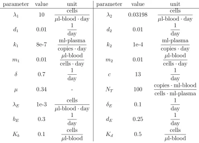
The values of model parameters (“true values”) used to generate the simulated data are given

in Table 1. The initial states were set to be 𝑥0 = (log10(800),log10(3.198),−4,−6,1,−2)𝑇.

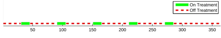
We simulated a treatment schedule for 364 days, with treatment off for the first 30 days, then alternating on for 15 days and off for 45 days, and then off treatment for the last 34 days of the year. This is shown in Figure 1, and also appears at the bottom of every graph of

100 150 200 250 300 350

50

On Treatment Off Treatment

Figure 1: The treatment schedule used in the experiments.

(12)

parameter value unit parameter value unit

𝜆1 10

cells

𝜇l-blood⋅day 𝜆2 0.03198

cells

𝜇l-blood⋅day

𝑑1 0.01 1

day 𝑑2 0.01

1 day

𝑘1 8e-7 ml-plasma

copies⋅day 𝑘2 1e-4

ml-plasma

copies⋅day

𝑚1 0.01

𝜇l-blood

cells⋅day 𝑚2 0.01

𝜇l-blood

cells⋅day

𝛿 0.7 1

day 𝑐 13

1 day

𝜇 0.34 - 𝑁𝑇 100 copies⋅ml-blood

cells⋅ml-plasma

𝜆𝐸 1e-3 cells

𝜇l-blood⋅day 𝛿𝐸 0.1

1 day

𝑏𝐸 0.3

1

day 𝑑𝐸 0.25

1 day

𝐾𝑏 0.1

cells

𝜇l-blood 𝐾𝑑 0.5

cells

𝜇l-blood

Table 1: Values of parameters in the HIV model.

3.2 Examination of Simulation Results

We will examine the observed states average RMS error deﬁned in (12) as well as the model compartments average RMS error deﬁned in (11), each when measurement data is taken 1 day, 7 days, 14 days or 28 days apart, respectively. Each of the simulated data sets for a

given sampling frequency was taken from the same 𝑁 “true” data sets, but taken at the

speciﬁed measurement frequency.

In order to test the ﬁlters under “poor” starting conditions with relatively uncertainty, we set ˆ𝑥𝑡0

𝑡0 = 0.6𝑥0 and P

𝑡0

𝑡0 = 0.01I for all the simulation results presented in this section. In

both the UKF and GHF, we set 𝛿𝑡= 0.005 in the discretization scheme (4). In some of our

(13)

3.2.1 State Estimation

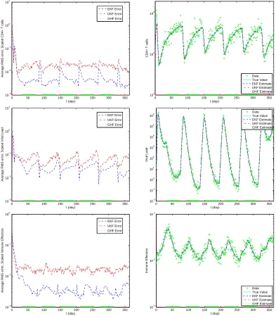
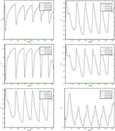
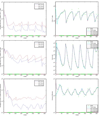
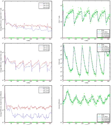
In this section, numerical results are obtained by applying the filtering algorithms to model (8) with measurements taken 1 day, 7 days, 14 days and 28 days apart. The plots in the left column of Figures 2 and 5 are for the average RMS error for each observed state defined by (12), and the ones in the right column are plotted for the estimated values versus the true values of the total CD4+ T-cell count, viral load level and immune effector T-cell count obtained by applying the filters to a typical data set. In addition, we have included the plots in Figures 3 and 6 for the average RMS error of each model compartment defined by (11).

Figures 4 and 7 contain the plots for the estimated values versus the true values of 𝑇1, 𝑇2,

𝑇∗

1, 𝑇2∗, 𝑉𝐼 and 𝐸 obtained by applying the ﬁlters to a typical data set.

(14)

0 50 100 150 200 250 300 350

10−3

10−2

10−1

100

101

t (day)

Average RMS error, Scaled CD4+ T cells

EKF Error UKF Error

GHF Error

0 50 100 150 200 250 300 350

101

102

103

t (day)

CD4+ T cells

Data True Value EKF Estimate UKF Estimate GHF Estimate

0 50 100 150 200 250 300 350

10−3

10−2

10−1

100

101

t (day)

Average RMS error, Scaled Viral Load

EKF Error UKF Error

GHF Error

0 50 100 150 200 250 300 350

10−2

10−1

100

101

102

103

104

105

106

t (day)

Viral Load

0 50 100 150 200 250 300 350

10−3

10−2

10−1

100

t (day)

Average RMS error, Scaled Immune Effectors

EKF Error UKF Error

GHF Error

0 50 100 150 200 250 300 350

10−3

10−2

10−1

t (day)

Immune Effectors

(15)

0 50 100 150 200 250 300 350

10−3

10−2

10−1

100

t (day)

Average RMS error, Scaled T

1

EKF Error UKF Error GHF Error

0 50 100 150 200 250 300 350

10−3

10−2

10−1

100

t (day)

1

*

0 50 100 150 200 250 300 350

10−3

10−2

10−1

100

t (day)

2

0 50 100 150 200 250 300 350

10−4

10−3

10−2

10−1

100

t (day)

2

*

0 50 100 150 200 250 300 350

10−3

10−2

10−1

t (day)

Average RMS error, Scaled V

I

0 50 100 150 200 250 300 350

10−3

10−2

10−1

t (day)

Average RMS error, Scaled E

(16)

0 50 100 150 200 250 300 350 101

102

t (day)

T1

True Value EKF Estimate UKF Estimate GHF Estimate

0 50 100 150 200 250 300 350 10−6

10−5 10−4 10−3 10−2 10−1 100 101 102

t (day)

T1

*

0 50 100 150 200 250 300 350 10−4

10−3 10−2 10−1 100

t (day)

T2

0 50 100 150 200 250 300 350 10−6

10−5 10−4 10−3 10−2 10−1 100

t (day)

T2

*

0 50 100 150 200 250 300 350 10−2

10−1 100 101 102 103 104 105 106

t (day)

VI

0 50 100 150 200 250 300 350 10−2

t (day)

E

(17)

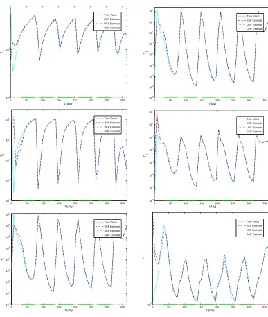
Figures 5, 6 and 7 illustrate the results obtained in the case when measurements are taken 7 days apart. Even though Figures 5 and 6 reveal that the UKF and GHF appear to adjust to the data slightly faster than the EKF, the average RMS errors obtained by the EKF for both observed states and model compartments are much smaller than those obtained by the UKF and GHF after day 100. Hence, for this measurement frequency, the EKF still performs much better than the UKF or the GHF. Also we observe that there is still no detectable diﬀerence in the estimation accuracy between the GHF and UKF. In addition, Figures 5 and 7 demonstrate that that all ﬁlters still perform well in estimating the observed states and each model compartment.

We have also applied the ﬁlters to the case with measurements taken 14 days and 28 days apart (sample results are given in the Appendix), and obtained the same conclusions as

those for measurements taken 1 day and 7 days apart. That is, for the case withonly model

states estimated, the EKF performs much better than both the UKF and GHF in terms of estimation accuracy for all the measurement frequencies that we have investigated, and there is little diﬀerence in the estimation accuracy between the UKF and GHF.

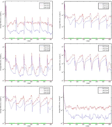
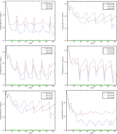
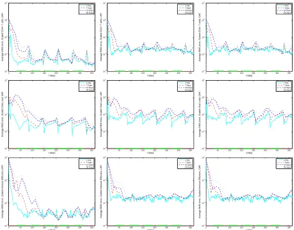
Figure 8 depicts the results for the average RMS error of each observed state with several dif-ferent measurement frequencies, where the plots in the left column, middle column and right column are the results obtained by using the EKF, UKF and GHF, respectively. From this figure, we see that the measurement frequency has no significant effect on the performance of the filters after day 100 (that is, after the filters adjust to the data). This is probably because for this case the nonlinearity is not so severe.

3.2.2 State and Parameter Estimation

Figures 9, 12, 15 and 18 were obtained by estimating parameters𝜆1 and𝑁𝑇 as well as model

states (i.e., the filters are applied to model (10)), where the figures in the left column are for the average RMS error of each observed state, and those in the right column are plotted for the estimated values versus the true values of the total CD4+ T-cell count, viral load level and immune effector T-cell count obtained by applying the filters to a typical data set. In addition, we have included the plots in Figures 10, 13, 16 and 19 for the average RMS error of each model compartment as well as each estimated parameter. Figures 11, 14, 17

and 20 contain the plots for the estimated values versus the true values of 𝑇1,𝑇2,𝑇1∗,𝑇2∗, 𝑉𝐼

and 𝐸 obtained by applying the ﬁlters to a typical data set. The results presented in this

section are typical for diﬀerent combinations of parameters that we estimated in a number of simulation studies.

(18)

0 50 100 150 200 250 300 350

10−3

10−2

10−1

100

101

t (day)

EKF Error

UKF Error GHF Error

0 50 100 150 200 250 300 350

101

102

103

t (day)

CD4+ T cells

0 50 100 150 200 250 300 350

10−3

10−2

10−1

100

101

t (day)

EKF Error

UKF Error GHF Error

0 50 100 150 200 250 300 350

10−2

10−1

100

101

102

103

104

105

106

t (day)

Viral Load

0 50 100 150 200 250 300 350

10−3

10−2

10−1

100

t (day)

EKF Error

UKF Error GHF Error

0 50 100 150 200 250 300 350

10−3

10−2

10−1

t (day)

Immune Effectors

Figure 5: State estimation with measurements 7 days apart. (left): average RMS error for each observed state; (right): the estimated values versus the true values for the total CD4+ T-cell count, viral load level and immune eﬀector T-cell count obtained by applying the ﬁlters to a typical data set.

(19)

0 50 100 150 200 250 300 350

10−3

10−2

10−1

100

t (day)

1

0 50 100 150 200 250 300 350

10−3

10−2

10−1

100

t (day)

1

*

0 50 100 150 200 250 300 350

10−3

10−2

10−1

100

t (day)

2

0 50 100 150 200 250 300 350

10−3

10−2

10−1

100

t (day)

2

*

0 50 100 150 200 250 300 350

10−3

10−2

10−1

100

t (day)

I

0 50 100 150 200 250 300 350

10−3

10−2

10−1

t (day)

(20)

0 50 100 150 200 250 300 350 101

102

t (day)

T1

0 50 100 150 200 250 300 350 10−6

10−5 10−4 10−3 10−2 10−1 100 101 102

t (day)

T1

*

0 50 100 150 200 250 300 350 10−4

10−3 10−2 10−1 100

t (day)

T2

0 50 100 150 200 250 300 350 10−6

10−5 10−4 10−3 10−2 10−1 100 101

t (day)

T2

*

0 50 100 150 200 250 300 350 10−2

10−1 100 101 102 103 104 105 106

t (day)

VI

0 50 100 150 200 250 300 350 10−2

t (day)

E

(21)