Volume 2008, Article ID 849040,10pages doi:10.1155/2008/849040
Research Article
Nonparametric Single-Trial EEG Feature Extraction and
Classification of Driver’s Cognitive Responses
Chin-Teng Lin,1Ken-Li Lin,1, 2Li-Wei Ko,1Sheng-Fu Liang,3Bor-Chen Kuo,4and I-Fang Chung5
1Department of Electrical and Control Engineering and Brain Research Center, National Chiao-Tung University, 1001 Ta Hsueh Road, Hsinchu 300, Taiwan
2Computer Center of Chung Hua University, Hsinchu 707, Section 2, WuFu Road, HsinChu 300, Taiwan
3Department of Computer Science and Information Engineering, National Cheng-Kung University, No. 1, University Road, Tainan 701, Taiwan
4Graduate Institute of Educational Measurement and Statistics, National Taichung University, 140 Min-Shen Road, Taichung 40306, Taiwan
5Institute of Biomedical Informatics, National Yang-Ming University, No. 155, Section 2, Linong Street, Taipei 112, Taiwan
Correspondence should be addressed to I-Fang Chung,[email protected]
Received 1 December 2007; Accepted 10 March 2008
Recommended by Chien-Cheng Lee
We proposed an electroencephalographic (EEG) signal analysis approach to investigate the driver’s cognitive response to traffi c-light experiments in a virtual-reality-(VR-) based simulated driving environment. EEG signals are digitally sampled and then transformed by three different feature extraction methods including nonparametric weighted feature extraction (NWFE), principal component analysis (PCA), and linear discriminant analysis (LDA), which were also used to reduce the feature dimension and project the measured EEG signals to a feature space spanned by their eigenvectors. After that, the mapped data could be classified with fewer features and their classification results were compared by utilizing two different classifiers includingknearest neighbor classification (KNNC) and naive bayes classifier (NBC). Experimental data were collected from 6 subjects and the results show that NWFE+NBC gives the best classification accuracy ranging from 71%∼77%, which is over 10%∼24% higher than LDA+KNN1. It also demonstrates the feasibility of detecting and analyzing single-trial EEG signals that represent operators’ cognitive states and responses to task events.
Copyright © 2008 Chin-Teng Lin et al. This is an open access article distributed under the Creative Commons Attribution License, which permits unrestricted use, distribution, and reproduction in any medium, provided the original work is properly cited.
1. INTRODUCTION
Global urbanization, increases in urban populations, urban sprawl, the growth of “mega-cities,” and the unrelenting increases in traffic around the world have created renewed concern about driving safety due to the growing number of traffic fatalities. Among these incidents, the fatalities are frequently caused by drivers’ failure to perceive changes in traffic lights or unexpected conditions occurring on the roads. Preventing such accidents is thus a major focus of efforts in the field of active safety research and healthcare sys-tems in vehicles. Early detection and recognition of driver’s cognitive response could be helpful in giving precautious alarms or providing some preventive actions.
In recent studies [1–3], many researchers proposed to develop quantitative techniques for ongoing assessment of cognitive effort, engagement, and workload, by
feasible. Based on Bayliss and Ballard’s experimental design concept, we have also developed methods in our previous paper [9] for analyzing single-trial electrical recordings from the human scalp in traffic light experiments and have proved the efficacy. In this paper, we further simplified and refined the methodology for quantitative analysis for ongoing assess-ment of driver’s cognitive responses by directly utilizing electroencephalographic (EEG) signals to investigate the neurobiological information underlying brain dynamics in traffic-light experiments in a virtual-reality (VR)-based simulated driving environment. Here, there is an important discrepancy between these two papers: the data collection process in this paper was modified by directly accessing brain signals originating in one channel of the visual region of the brain. Hence, we did not need to use blind source separation technique like independent component analysis (ICA) as adopted in our previous paper. This approach can eliminate the necessity of offline manual selection of desired source component such that online classification is possible and desirable in the sense of practical applications.
In order to reduce the feature dimension of EEG signals, some studies have shown that parametric feature extraction methods are successfully applied to EEG signal analyses [10– 12] and nonparametric feature extraction method proposed by one member of our research team is also proved the appli-cation on the recognition of satellite images [13]. Hence, after obtaining the EEG signals, refinement of analysis in this paper was first achieved by comparing data produced from three different feature extraction methods including nonparametric weighted feature extraction (NWFE), princi-pal component analysis (PCA), linear discriminant analysis (LDA), which were applied to reduce the feature dimension and project the measured EEG signals to a feature space spanned by their eigenvectors. After that, the mapped data could be classified with fewer features and their classification results are compared by utilizing two different classifiers including k nearest neighbor classification (KNNC) and naive bayes classifier (NBC). It should be noted that since we want to put emphasis on the efficacy comparison between the nonparametric and parametric feature extraction methods, we adopted two simple classifiers (KNNC and NBC) to avoid the good prediction results obtained mainly owing to adopt-ing a complicated classifier even though Garrett et al. show that nonlinear classifiers produces slightly better prediction results for the classification of spontaneous EEG signals [14].
2. SYSTEM ARCHITECTURE
2.1. Virtual reality-(VR-) based driving environment
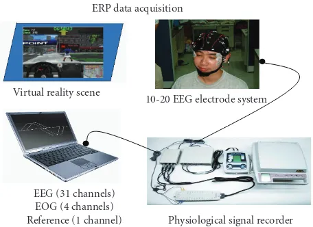
To explore brain activities in the safety-driving system, this experiment was designed to detect and analyze the event related potential (ERP) signals of brain activities related to traffic light events (Red-Green-Yellow) since they are the most frequent events when driving on the roads and highly correlated to the traffic accidents. The overall experiment environment included various simulated events shown in Figure 1: (1) a visual display unit to provide the simulated events, (2) EEG measurement system with 36-channel EEG
ERP data acquisition
Virtual reality scene
10-20 EEG electrode system
EEG (31 channels) EOG (4 channels)
Reference (1 channel) Physiological signal recorder Figure1: Physiological signal measurement system in the VR-based traffic-light simulation experiments.
head mounted sensors, and (3) spatial and temporal signal processing technologies based on several kinds of feature extraction and classification methods. Figure 2 shows the flowchart of EEG signal processing and analysis. EEG signals are digitally sampled and one among these channels is selected for classification task. Each dataset for one subject was shuffled and randomly divided into 4 subdatasets to do 4-fold cross-validation. In each cross-validation stage it includes 4 runs. Each run will use 3 subdatasets for training and the remaining one subdataset for testing. Labeling the subdatasets from 1 to 4, then the training data used in each run would be{2, 3, 4}, {1, 3, 4}, {1, 2, 4}, and{1, 2, 3}, respectively, while the test data are{1}, {2}, {3}, and{4}, accordingly. The average accuracy of the 4 runs is calculated as the result of this cross-validation stage. Such processes were repeated 10 times to get the average accuracy and standard deviation to decrease possible bias caused by any specific selected dataset. As shown in Figure 2, three dif-ferent feature extraction methods including nonparametric weighted feature extraction (NWFE), principal component analysis (PCA), and linear discriminant analysis (LDA) are used. After feature extraction process, the extracted features are classified by two different classifiers:k nearest neighbor classification (KNNC) and naive bayes classifier (NBC). The classification results of different combinations of features extraction approaches and classification methods are evaluated and compared.
2.2. Subjects and EEG data collection
EEG data preprocessing
EEG signals Channel selection
4-fold data splitting
Feature extraction Feature space transformation
PCA
NWFE
LDA
Classification
KNNC
NBC
Figure2: System flowchart for processing the EEG signals.
with a unipolar reference at the right earlobe), 2 ECG channels (bipolar connection) were simultaneously recorded by the Scan NuAmps Express system (Compumedics Ltd., VIC, Australia). All the EEG/EOG sensors were placed based on a modified international 10–20 system. Before data acquisition, the contact impedance between EEG electrodes and scalp was controlled to be less than 5 kΩ. The EEG data were recorded with 16-bit quantization level at a sampling rate up to 1 KHz. Then, EEG data were preprocessed using a simple low-pass filter with a cutofffrequency of 50 Hz to remove the line noise (60 Hz and its harmonic) and other high-frequency noise for further analysis.
3. FEATURE EXTRACTION AND CLASSIFICATION METHODS
To analyze the relation between EEG signals and the subjects’ response, we apply the three different feature extraction and classification methods on different channel signals. According to several experimental test runs, we select Pz as the target channel for classification. Though some other channels may yield similar level of classification accuracy such as Cz, however, our goal is focused on the sensory visual processing signal rather than others, so we make the decision to choose Pz channel.Figure 2shows the system flowchart for processing the EEG signals. The Pz channel EEG signals are processed through one of feature extraction methods among nonparametric weighted feature extraction (NWFE), principal component analysis (PCA), or linear discriminant analysis (LDA) to map the original data to feature vectors of reduced dimension. After that, the reduced features are fed into one of classifiers such as knearest neighbor classifier (kNNC) and naive bayes classifier (NBC) for comparison of classification accuracy. Each analysis method is described briefly in this section.
3.1. Nonparametric weighted feature extraction (NWFE)
NWFE is a nonparametric feature extraction [13]. The main ideals of NWFE are putting different weights on every sample to compute the “weighted means” and compute the distance between samples and their weighted means as
their “closeness” to boundary, then defining nonparametric between-class and within-class scatter matrices which put large weights on the samples close to the boundary and de-emphasize those samples far from the boundary. The between-class scatter matrixSNW
b and the within-class scatter
matrixSNW
w of NWFE are defined as
SNWb = L
i=1
Pi L
j=1
j /=i
Ni
k=1
λ(ki,j)
ni
xk(i)−Mj
x(ki)
x(ki)−Mj
xk(i)
T
,
SNW
w =
L
i=1
Pi Ni
k=1
λ(ki,i)
ni
x(ki)−Mi
xk(i)x(ki)−Mi
x(ki)T, (1)
whereMj(x(ki))=
Nj
l=1w (i,j)
kl x
(j)
l ,
λ(ki,j)=
distx(ki),Mj
xk(i)
−1
Nj
t=1dist
x(ti),Mj(x(ti)
−1,
w(kli,j)=
distxk(i),x(lj)−1
nj
t=1dist
x(ti),x
(j)
l
−1,
(2)
whereNidenotes the training sample size of classi, Lis the
number of classes,Piis a prior probability of classi, x(li)is
thelth sample of classi, Mj(xl(i)) denotes the weighted mean
ofxl(i)in classj, and dist(x,z) is the Euclidean distance from
xtoz. If the distance betweenxk(i)andMj(x(ki)) is small, then
its weightλ(ki,j)will be close to 1; otherwise,λ
(i,j)
k will be close
to 0. The sum of theλ(ki,j)for classiis 1. The weightw
(i,j)
kl
for computing weighted means is a function ofx(ki)andxl(j). If the distance betweenx(ki)andx
(j)
l is small then its weight
wkl(i,j)will be close to 1; otherwise,w(kli,j)will be close to 0. The sum of thewkl(i,j)forMj(x(ki)) is 1.
problem. This is in contrast to linear discriminant analysis (LDA), which usually only can extract L−1 (number of classes minus one) features. In a real situation, this may not be enough. Second, the nonparametric nature of scatter matrices reduces the effects of outliers and works well even for nonnormal datasets. NWFE provides greater weight to samples near the expected decision boundary. This tends to provide for increased classification accuracy.
3.2. Principlal component analysis (PCA)
The goal of PCA is to find a set ofp≤dvectors inRdspace
containing the maximum amount of variance in the data. Suppose that the data has been centered in the original space andνis an arbitrary normalized vector inRd. The variance
of the projections of the all pixels xj onto this normalized
directionνis
1
N
N
j=1
νTx
jxTjν=νT
1
N
N
j=1
xjxTj
ν=νTCν, (3)
whereCis thed×dcovariance matrix and defined by
C= 1
N
N
j=1
xjxTj. (4)
The first principal vector can be found by the following equation:
ν= arg max
ν∈Rd,ν =1
νTCν. (5)
The solution of the above equation is the eigenvector ν of C with respect to the largest eigenvalue. One can seek for the direction of second largest variance in the orthogonal subspace, by looking for the largest eigenvector in the matrix obtained by deflating the matrixCwith respect toν. Repeating this step shows that the mutually orthogonal directions of maximum variance in order of decreasing size are given by the eigenvectors ofC.
3.3. Linear discriminant analysis (LDA)
LDA is often used for dimension reduction in classification problems. It is also called the parametric feature extraction method in [15], since LDA uses the mean vector and covari-ance matrix of each class. Usually within-class, between class, and mixture scatter matrices are used to formulate the criterion of class separability. A within-class scatter matrix forLclasses is expressed by
SLDA
w =
L
i=1
PiΣi= L
i=1
PiSLDAwi , (6)
where Pi denotes the prior probability of class iand Σi is
the class covariance matrix. A between-class scatter matrix is expressed as
SLDA
b =
Pi
mi−m0
mi−m0
T
= L−1
i=1
L
j=i+1
PiPj
mi−mj
mi−mj
T
,
(7)
wheremiis the class mean andm0 represents the expected
vector of the mixture distribution and is given by
m0=
L
i=1
Pimi. (8)
The optimal features are determined by optimizing the Fisher criterion given by
JLDA=tr
SLDA
w
−1
SLDA
b . (9)
This is equivalent to solve the following generalized eigen-value problem and the extracted eigenvectors are formed the transformation matrix of LDA,
SLDAb ν=λSLDAw ν. (10)
3.4. Classifiers
In this study, two types of classifiers are used.
(i)knearest neighbor classification (kNNC) is a simple and appealing approach in pattern recognition. k
nearest neighbor classifier finds the set ofk nearest neighbors in the training set to a testing sample,x, and then classifiesxas the most frequent class among the k neighbors. The search of nearest neighbors is a flexible classification scheme, and does not involve any preprocessing or fitting of the training data. Hence,knearest neighbor classifier belongs to nonparametric classifiers. The detailed definition of nearest neighbor classification is described as in [15]. In this paper, the parameterk is set to 1 or 3 and the classifiers are denoted as KNN1 or KNN3 in the following paragraphs.
(ii) Naive bayes classifier (NBC) is also a simple approach in pattern recognition. Based on Bayesian theorem and assumption of independence of attributes, NBC tries to appoint a sample x with attribute values (A1 = ν1, A2 = ν2,. . ., An = νn) to class Ci
with maximum a posterior probability (MAP) for all classesi,
c∗=arg max
i Prob
Ci|
ν1,ν2,. . .,νn
=arg max
i
Pν1,ν2,. . .,νn
|Ci
PCi
Pν1,ν2,. . .,νn
=arg max
i P
ν1,ν2,. . .,νn
|Ci
PCi
=arg max
i n
h=1
Pνh|Ci
PCi
,
(11)
whereP(νh | Ci) is the probability of the attribute
Ah =νh given the classCiandP(Ci) is the number
of training samples belonging to class Ci. Due to
3.5. Performance measure
Two performance measures are used for the evaluation of classification result. One is commonly used average classification accuracy, which is defined as
Pa=
Ncorrect
Ntotal
, (12)
whereNcorrect is the number of correctly predicted samples
andNtotalis the number of all testing samples.
The other performance measure is Kappa coefficient, also known as Cohen’s Kappa or kappa statistic [16]. The Kappa coefficient value is ranged between 1 and−1, which corresponds to a perfect and a completely wrong classi-fication, respectively. And Kappa coefficient with value 0 means random guess performance. Following the derivation of Kappa [17], it can be calculated as follows;
K=
Po−Pe
1−Pe
, (13)
wherePodenotes the proportion of overall agreement andPe
is the proportion of chance expected agreement.
4. EXPERIMENT RESULTS
In our experiment, a subject simulated driving a car using the VR-based ERP experimental system described inSection 2. The continuous EEG signals measured from the EEG sensors were first separated into several epochs/trials. For this exper-iment, an epoch or a trial was defined as containing the sam-pled data from –200 millseconds to 1000 millisecondss when a light event was given at 0 millisecond. The objective of this experiment was to detect and evaluate cognitive responses of the driver to traffic-light events by directly accessing brain signals originating in one channel of the visual region of the brain. Each EEG trial originally containing 1200 recorded values taken at intervals of 1200 milliseconds was down-sampled by picking up the first sample of every 3 data points (3 milliseconds) to form one 400-dimension sample vector. The down-sampled EEG trials of every participant form the dataset for training and testing and each trial is classified into one of the red, green, or yellow light events (i.e., the number of class labels L = 3). Each dataset for one subject was shuffled and randomly divided into 4 subdatasets to do 4-fold cross-validation. Such processes were repeated 10 times to get the average accuracy and standard deviation to decrease possible bias caused by any specific selected dataset. Moreover, in order to increase computational efficiency, we applied three different feature extraction techniques to the dataset, including NWFE, PCA, and LDA. After feature extraction, the 400-dimension sample vectors for each participant were mapped to the feature space and the top one to fifty transformed features were chosen for testing optimal classification accuracy by observing the Kappa coefficients.
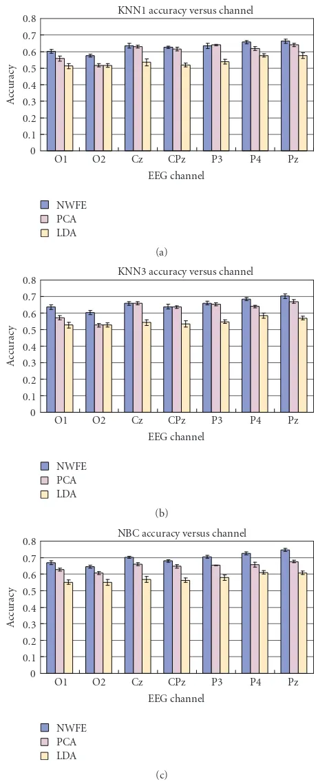
In performing the experiments, first, we evaluated how different EEG channels influence the classification accuracy. In order to find the channel most related to visual cognitive
Pz P4 P3 CPz Cz O2 O1
EEG channel NWFE
PCA LDA 0 0.1 0.2 0.3 0.4 0.5 0.6 0.7 0.8
A
ccur
acy
KNN1 accuracy versus channel
(a)
Pz P4 P3 CPz Cz O2 O1
EEG channel NWFE
PCA LDA 0 0.1 0.2 0.3 0.4 0.5 0.6 0.7 0.8
A
ccur
acy
KNN3 accuracy versus channel
(b)
Pz P4 P3 CPz Cz O2 O1
EEG channel NWFE
PCA LDA 0 0.1 0.2 0.3 0.4 0.5 0.6 0.7 0.8
A
ccur
acy
NBC accuracy versus channel
(c)
Figure3: Accuracy plot for different EEG channels.
NBC KNN3
KNN1 0.4
0.45 0.5 0.55 0.6 0.65 0.7 0.75 0.8
A
ccur
acy
Subject 1
(a)
NBC KNN3
KNN1 0.4
0.45 0.5 0.55 0.6 0.65 0.7 0.75 0.8
A
ccur
acy
Subject 2
(b)
NBC KNN3
KNN1 0.4
0.45 0.5 0.55 0.6 0.65 0.7 0.75 0.8
A
ccur
acy
Subject 3
(c)
NBC KNN3
KNN1 0.4
0.45 0.5 0.55 0.6 0.65 0.7 0.75 0.8
A
ccur
acy
Subject 4
(d)
NBC KNN3
KNN1 0.4
0.45 0.5 0.55 0.6 0.65 0.7 0.75 0.8
A
ccur
acy
Subject 5
NWFE PCA LDA
(e)
NBC KNN3
KNN1 0.4
0.45 0.5 0.55 0.6 0.65 0.7 0.75 0.8
A
ccur
acy
Subject 6
NWFE PCA LDA
(f)
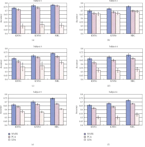
Figure4: Classification results for six different subjects based on EEG signals from Pz channel.
performed best overall in more accurately predicting the cog-nitive response. For the NWFE and PCA feature extraction methods, Figure 3 shows that the Pz channel consistently performed best. Only for the LDA feature extraction method did the P4 channel perform better, but such performance was only marginally better. The same can be observed for the KNN3 and NBC classifiers (with the exception for the Cz channel for the KNN3 method, which performed on a par with the Pz channel). Consequently, in the subsequent test cases, we chose the measured signals of the Pz channel to be the feature vectors for classification.
any one of the classifiers produced the lowest accuracy, and in some instances, substantially poorer accuracy. It is possible that LDA itself can act as a classifier (e.g., use Fisher’s classification functions) and its performance as a classifier might be better than using the LD scores into a different classifier. The PCA feature extraction method, combined with any of the classifiers, produced results consistently better than the LDA method, but less accurate (and in some cases significantly less accurate) than the NWFE method. Table 1 contains amplification of the data fromFigure 4, supplying in addition the standard deviation for accuracy for each subject by each method,and also the numbers of features used. Also as can be seen in Table 1, the NWFE method effectively reduces the number of features from 400 down to 2. Since the amplitudes of single-trial ERP signals are far weaker than the ongoing EEG signals, proper feature extraction before classification can increase the accuracy and reduce the data dimension to save the training and processing time for online analysis system.
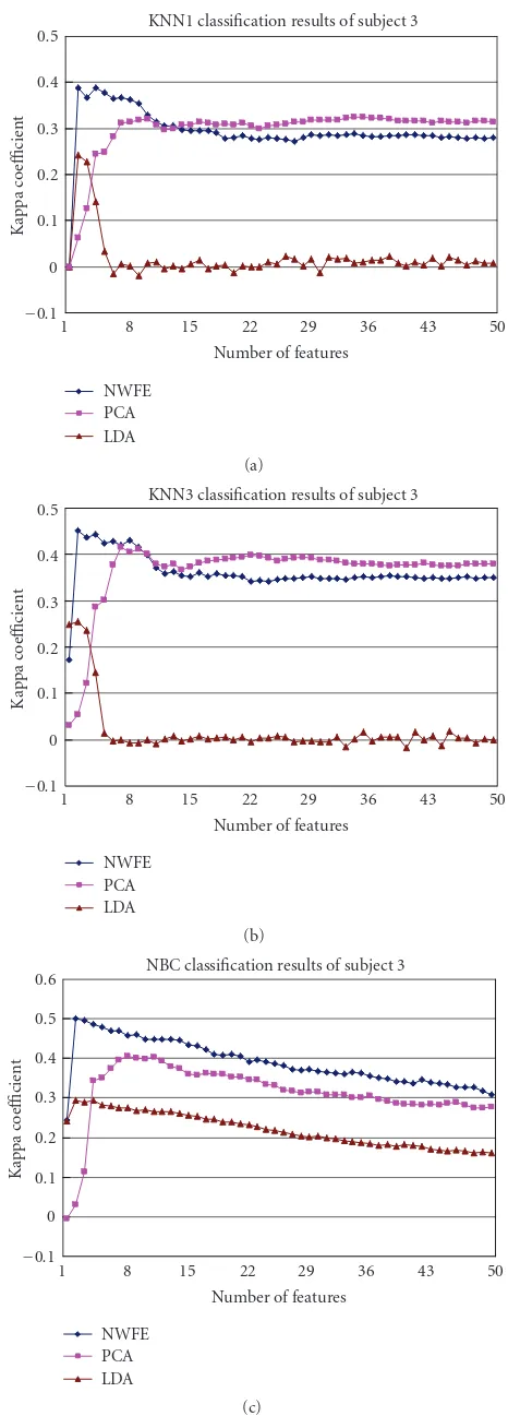
In order to confirm the efficacy of the NWFE feature extraction method, when used with any classifier, the same data was analyzed using an alternative index, Kappa coefficient. Figure 5 shows the Kappa coefficient versus a range of features for Subject 3 using different classifiers. The x-axis ranging from 1 to 50 represents the number of features used for classification after feature reduction, and they-axis represents the Kappa coefficient. A higher Kappa coefficient indicates higher accuracy.Figure 5offers further corroboration that NWFE obtains better accuracy than other methods, especially when using fewer features. It is noted that as feature numbers increase, initially the accuracy also increases, but after best accuracy achieved by using a certain number of features, the accuracy begins to decrease when more features are used. Also,different classifiers differ somewhat in how the accuracy decreases [18].
In the previous VR-based stop light experiment without the dynamic platform [7], the recognition results between two lights (red/yellow) were 67% to 73% in average of five subjects with different algorithms. In our past study, we acquired 31-channel whole head EEG signals to recognize traffic-light visual ERP [9]. The recognition sensitivity can achieve 79% to 95% by combining independent component analysis (ICA), PCA, and self-constructing neural fuzzy inference network (SONFIN). In this study, we utilize NWFE to extract features from one channel single-trial EEG data and use NBC for classification. It can achieve up to 77% accuracy in traffic-light visual ERP classification. Since only one EEG channel is used, the preparation time for electrode placement, skin preparation, and gel application as well as the system complexity can be greatly reduced. It is more convenient for practical applications. On the other hand, the accuracy is possibly improved by some other choices of classifiers. For instance, we have some preliminary investigation by using the support vector machine (SVM) with RBF kernel to classify the ERPs of Subject 3 as an example. The accuracy of applying SVM to classify the features extracted by NWFE, PCA, and LDA is 74.87%, 72.86%, and 59.6%, respectively. The NWFE + SVM can also
50 43 36 29 22 15 8 1
Number of features NWFE
PCA LDA
−0.1 0 0.1 0.2 0.3 0.4 0.5
Ka
p
p
a
co
e
ffi
cient
KNN1 classification results of subject 3
(a)
50 43 36 29 22 15 8 1
Number of features NWFE
PCA LDA
−0.1 0 0.1 0.2 0.3 0.4 0.5
Ka
p
p
a
co
e
ffi
cient
KNN3 classification results of subject 3
(b)
50 43 36 29 22 15 8 1
Number of features NWFE
PCA LDA
−0.1 0 0.1 0.2 0.3 0.4 0.5 0.6
Ka
p
p
a
co
e
ffi
cient
NBC classification results of subject 3
(c)
200 100 0
−100
−200
Feature 1
−100
−50 0 50 100 150 200 250
Fe
at
u
re
2
Subject3-NWFE-train projection
150 100 50 0
−50
−100
Feature 1
−100
−50 0 50 100 150 200
Fe
at
u
re
2
Subject3-NWFE-test projection
(a) NWFE-mapped feature space
×102 20 10 0
−10
−20
Feature 1
−4
−3
−2
−1 0 1 2 3 4
×102
Fe
at
u
re
2
Subject3-PCA-train projection
×10102 5 0
−5
−10
Feature 1
−3
−2
−1 0 1 2 3
×102
Fe
at
u
re
2
Subject3-PCA-test projection
(b) PCA-mapped feature space
×10−3 2 1 0
−1
−2
Feature 1
−1.5
−1
−0.5 0 0.5 1 1.5
×10−3
Fe
at
u
re
2
Subject3-LDA-train projection
0.01 0.005 0
−0.005
−0.01
Feature 1
−1.5
−1
−0.5 0 0.5 1 1×.5
10−3
Fe
at
u
re
2
Subject3-LDA-test projection
(c) LDA-mapped feature space
Figure6: Scatter-plot for Subject 3 using (a) NWFE, (b) PCA, and (c) LDA methods.
achieve the best performance and is slightly better than the NWFE + NBC in this case.
To graphically visualize the difference of projected data spread in a reduced feature space, training, and testing data are projected into a 2-dimension feature space. Three scatter plots are shown in Figure 6(a) through Figure 6(c), where the left-hand side is the training data projection and the right-hand side is the test data projection. Three colors are used to indicate the three different EEG events (e.g., red, green, and yellow lights) and each focus indicates the center of each event distribution. From the Figures, NWFE and LDA both separate projected training data better than PCA, while NWFE also performs better than LDA for projected test data separation. The distinct separation of the three
event signals for both training and testing patterns shows the overall superiority of the NWFE method. That gives a visual interpretation for the classification results.
5. CONCLUSIONS
Table1: Classification results.
CL: classifier, Acc: accuracy, Fno: feature no. used
Feature extraction NWFE PCA LDA
Subject CL Acc Fno Acc Fno Acc Fno
Sub 1
KNN1 73.33%±0.97% 2 71.29%±1.18% 11 50.01%±2.73% 2
KNN3 76.51%±1.43% 3 73.78%±1.28% 11 52.04%±3.42% 3
NBC 77.37%±0.94% 2 76.26%±1.15% 3 50.95%±2.33% 8
Sub 2
KNN1 69.57%±1.89% 3 66.56%±1.62% 7 65.74%±2.10% 2
KNN3 72.50%±1.03% 2 68.13%±1.22% 32 66.60%±1.91% 2
NBC 75.50%±0.93% 2 69.54%±1.26% 11 68.77%±1.49% 1
Sub 3
KNN1 67.22%±0.98% 4 63.12%±1.49% 35 56.30%±5.16% 2
KNN3 70.69%±1.43% 2 68.61%±0.95% 7 57.81%±4.83% 2
NBC 73.84%±0.80% 2 69.63%±1.28% 8 61.92%±2.06% 4
Sub 4
KNN1 66.88%±1.50% 3 61.77%±1.77% 17 51.91%±2.42% 1
KNN3 69.02%±1.49% 3 64.91%±1.35% 20 51.57%±2.48% 1
NBC 71.66%±1.75% 6 67.28%±1.00% 4 53.05%±2.58% 1
Sub 5
KNN1 66.30%±1.27% 2 63.98%±1.04% 12 57.52%±1.64% 3
KNN3 70.25%±1.39% 2 67.03%±1.06% 22 57.03%±1.11% 2
NBC 74.53%±0.90% 2 67.60%±0.83% 13 60.79%±0.93% 1
Sub 6
KNN1 64.92%±1.71% 3 62.32%±0.93% 13 53.89%±1.90% 1
KNN3 67.41%±0.79% 2 65.73%±0.55% 12 54.80%±0.71% 3
NBC 71.40%±0.63% 2 68.21%±0.82% 7 57.14%±1.91% 1
environment consists of surrounded virtual reality scenes, a driving motion simulator, and the EEG signal acquisition system. Regarding comparison of classification results, we combined three well-known feature extraction methods with two different classifiers to classify the single-trial EEG signal of driver’s cognitive responses corresponding to different traffic-light events. Experimental results showed that NWFE could extract the fewer features (almost in 2 features) in each subject experiment to represent the EEG data distribution and then using NBC as the classifier could reach the better accuracy. In addition, since the proposed approach utilizes only one EEG channel, the preparation time for electrode placement, skin preparation, and gel application as well as the system complexity can be greatly reduced. It is feasible and desirable for practical applications.
ACKNOWLEDGMENTS
This work was supported in part by the National Science Council, Taiwan, under Contracts NSC 96-2627-E-009-001-and NSC 96-2218-E-009-001-, 96-2627-E-009-001-and in part by the “Aiming for the Top University Plan (ATU)” of the National Chiao-Tung University and the Ministry of Education (MOE), Taiwan, under Contract no. 97W806.
REFERENCES
[1] A. Kemeny and F. Panerai, “Evaluating perception in driving simulation experiments,”Trends in Cognitive Sciences, vol. 7, no. 1, pp. 31–37, 2003.
[2] Z. Duric, W. D. Gray, R. Heishman, et al., “Integrating perceptual and cognitive modeling for adaptive and intelligent
human-computer interaction,”Proceedings of the IEEE, vol. 90, no. 7, pp. 1272–1289, 2002.
[3] D. D. Schmorrow and A. A. Kruse, “DARPA’s augmented cognition program-tomorrow’s human computer interaction from vision to reality: building cognitively aware computa-tional systems,” inProceedings of the 7th IEEE Conference on Human Factors and Power Plants, pp. 7/1–7/4, Scottsdale, Ariz, USA, September 2002.
[4] P. Sykacek, S. J. Roberts, and M. Stokes, “Adaptive BCI based on variational Bayesian Kalman filtering: an empirical evaluation,” IEEE Transactions on Biomedical Engineering, vol. 51, no. 5, pp. 719–727, 2004.
[5] T. J. Dasey and E. Micheli-Tzanakou, “Detection of multiple sclerosis with visual evoked potentials—an unsupervised computational intelligence system,” IEEE Transactions on Information Technology in Biomedicine, vol. 4, no. 3, pp. 216– 224, 2000.
[6] X. Gao, D. Xu, M. Cheng, and S. Gao, “A BCI-based environ-mental controller for the motion-disabled,”IEEE Transactions on Neural Systems and Rehabilitation Engineering, vol. 11, no. 2, pp. 137–140, 2003.
[7] J. D. Bayliss and D. H. Ballard, “Single trial P3 epoch recog-nition in a virtual environment,”Neurocomputing, vol. 32-33, pp. 637–642, 2000.
[8] J. D. Bayliss and D. H. Ballard, “Recognizing evoked potentials in a virtual environment,” inAdvances in Neural Information Processing Systems 12, pp. 3–9, MIT Press, Cambridge, Mass, USA, 2000.
[9] C.-T. Lin, I.-F. Chung, L.-W. Ko, Y.-C. Chen, S.-F. Liang, and J.-R. Duann, “EEG-Based assessment of driver cognitive responses in a dynamic virtual-reality driving environment,”
IEEE Transactions on Biomedical Engineering, vol. 54, no. 7, pp. 1349–1352, 2007.
event-related potentials in the brain,” IEEE Transactions on Biomedical Engineering, vol. 35, no. 9, pp. 701–711, 1988. [11] J. Pardy, S. Roberts, and L. Tarassenko, “A review of parametric
modeling techniques for EEG analysis,”Medical Engineering & Physics, vol. 18, no. 1, pp. 2–11, 1996.
[12] D. P. Burke, S. P. Kelly, P. de Chazal, R. B. Reilly, and C. Finucane, “A parametric feature extraction and classification strategy for brain-computer interfacing,”IEEE Transactions on Neural Systems and Rehabilitation Engineering, vol. 13, no. 1, pp. 12–17, 2005.
[13] B.-C. Kuo and D. A. Landgrebe, “Nonparametric weighted feature extraction for classification,” IEEE Transactions on Geoscience and Remote Sensing, vol. 42, no. 5, pp. 1096–1105, 2004.
[14] D. Garrett, D. A. Peterson, C. W. Anderson, and M. H. Thaut, “Comparison of linear, nonlinear, feature selection methods for EEG signal classification,” IEEE Transactions on Neural Systems and Rehabilitation Engineering, vol. 11, no. 2, pp. 141– 144, 2003.
[15] K. Fukunaga,Introduction to Statistical Pattern Recognition, chapters 9-10, Academic Press, San Diego, Calif, USA, 1990. [16] H. C. Kraemer,Encyclopedia of Statistical Science, John Wiley
& Sons, New York, NY, USA, 1982.
[17] G. Townsend, B. Graimann, and G. Pfurtscheller, “A compar-ison of common spatial patterns with complex band power features in a four-class BCI experiment,”IEEE Transactions on Biomedical Engineering, vol. 53, no. 4, pp. 642–651, 2006. [18] T. Howley, M. G. Madden, M.-L. O’Connell, and A. G. Ryder,