Volume 2009, Article ID 293952,19pages doi:10.1155/2009/293952
Research Article
Multiresolution Analysis Adapted to Irregularly Spaced Data
Anissa Mokraoui
1and Pierre Duhamel (EURASIP Member)
21L2TI, Institut Galil´ee, Universit´e Paris 13, 99, Avenue Jean Baptiste Cl´ement, 93 430 Villetaneuse, France 2LSS/CNRS, SUPELEC, Plateau de Moulon, 91 192 Gif sur Yvette, France
Correspondence should be addressed to Anissa Mokraoui,[email protected]
Received 26 February 2009; Revised 18 July 2009; Accepted 18 September 2009
Recommended by Enrico Capobianco
This paper investigates the mathematical background of multiresolution analysis in the specific context where the signal is represented by irregularly sampled data at known locations. The study is related to the construction of nested piecewise polynomial multiresolution spaces represented by their corresponding orthonormal bases. Using simple spline basis orthonormalization procedures involves the construction of a large family of orthonormal spline scaling bases defined on consecutive bounded intervals. However, if no more additional conditions than those coming from multiresolution are imposed on each bounded interval, the orthonormal basis is represented by a set of discontinuous scaling functions. The spline wavelet basis also has the same problem. Moreover, the dimension of the corresponding wavelet basis increases with the spline degree. An appropriate orthonormalization procedure of the basic spline space basis, whatever the degree of the spline, allows us to (i) provide continuous scaling and wavelet functions, (ii) reduce the number of wavelets to only one, and (iii) reduce the complexity of the filter bank. Examples of the multiresolution implementations illustrate that the main important features of the traditional multiresolution are also satisfied.
Copyright © 2009 A. Mokraoui and P. Duhamel. This is an open access article distributed under the Creative Commons Attribution License, which permits unrestricted use, distribution, and reproduction in any medium, provided the original work is properly cited.
1. Introduction
Multiresolution theory has been extensively studied for more than a decade (see, e.g., [1–4]). Initially, the multiresolution theory has been mainly developed within the framework of samples taken at regular sampling instants. Therefore the scaling and wavelet bases are built under the assumptions that the knots associated to the discrete signal are regularly spaced. The scaling or wavelet basis is defined as a set of translations and dilations of a single prototype function. Thus, the obtained functions are similar to each other at different scales.
However, the nonuniform sampling situation arises nat-urally in many scientific fields such as geophysics, astronomy, meteorology, medical imaging and computer vision where data are often generated or measured at sparse and irregular known positions. In the literature few works are available in this context, compared to those developed in the case of regularly spaced data. It is within this framework that we have concentrated our study. The proposed approach can be used to interpolate irregularly sampled signals in an efficient way, by keeping the multiresolution strategy.
The nonequally spaced data assumption results in a more general definition of the scaling and wavelet functions. The development of the scaling and wavelet bases, provided in this paper, focuses on piecewise polynomials, named nonuniform B-spline functions. These functions are widely used to model curves and surfaces in computer graphics [5]. The spline functions were already successfully used in the uniform spacing knot case leading to the construc-tion of spline scaling and wavelet funcconstruc-tions. An extensive bibliography is available (see, e.g., [6–10]), while rela-tively little works have been published about the construc-tion of these funcconstruc-tions on arbitrary nonuniformly spaced knots.
The authors of [11], review and discuss some techniques and tools for constructing wavelets on an irregular set of points by means of generalized subdivision schemes and commutation rules. They have adapted Lemari´e’s commu-tation formula to an irregular setting [12]. Starting from a coarse and irregular set of points, the subdivision technique consists in iterating the upsampling process using a local averaging function to refine and control the shape of a curve. In this case, the wavelet and scaling functions from the coarsest level are generated with a subdivision scheme using new points provided by the finest level grid on which the data was initially sampled. However, smoothness results in these settings become much harder to obtain.
This strategy has been widely used in the two dimen-sional case based on the triangulation plane of a function [19] which is also based on the formalism of a commutation approach for an irregular subdivision scheme. The authors of reference [13] proposed as a sequel of paper [11] the construction of an entire family of biorthogonal compactly supported irregular knot B-spline wavelets.
In reference [15], Buhmann and Micchelli originally presented a theoretical study to perform a multiresolution analysis using spline spaces of arbitrary degree adapted to nonuniform knot sequences. They proposed a generalization of the cardinal spline approach to the wavelets which have been extensively studied in the uniform spaced data case [3]. The proposed wavelet (named prewavelet in their paper) is given as the (n+ 1)th order derivative of the spline function of degree 2n+ 1. The existence of compactly supported wavelets which decay exponentially has been shown. The support of the wavelet depends on the degree n of the spline function and is given by the interval [xi,xi+2n+1]
(wherexk specifies the data position). Moreover, Buhmann
and Micchelli proved that the insertion ofLmultiple knots between two consecutive knots belonging to the previous coarse scale involves 2n+Lwavelets.
On another hand, the authors of paper [14] investigated the construction of a semiorthogonal spline wavelet basis for nonuniform partitions on a bounded interval. They proposed the construction of nonuniform B-spline functions with multiple knots at each end point of the interval as special boundary functions. They provided explicit expres-sions of the nonuniform B-spline wavelets. Decomposition and reconstruction algorithms using filter banks are also proposed. However the dimension of the spline wavelet space increases with the insertion of knots from one resolution level to another. This situation increases the computational complexity of the filter bank and moreover its implementation.
In [17], Wang focused on the construction of com-pactly supported wavelets on arbitrary partitions where additional conditions were imposed on the end-points of the cubic spline thereby obtaining a unique interpolating cubic spline.
In [20], the spline basis orthonormalization process used for constructing the orthonormal scaling and wavelet bases, is defined separately on each bounded interval of the knots sequence. This process introduces discontinuities of the spline scaling functions at each end-point of the intervals.
The resulting spline wavelet basis functions are also affected. The wavelet functions are not only discontinuous at each end-point of the nonuniform B-spline intervals but are also inside each interval. Moreover, the dimension of the spline wavelet space is proportional to the degree of the spline function.
In the framework of this paper, we have chosen to work separately on each bounded interval of the real line and to impose multiplicities of maximal order at end-points of the B-spline function definition domain [21]. The generated piecewise polynomial spaces allow an obvious scaling of the spaces as required for a multiresolution construction. Indeed, a piecewise polynomial of a given degree over a bounded interval at any resolution level is also a piecewise polynomial at another resolution level. Moreover, many simple bases can be built for such piecewise polynomial spaces.
The main objective of this paper is to propose a basis orthonormalization procedure which allows for the construction of suitable bases of the spline scaling and wavelet spaces ensuring the continuities of all functions whatever the degree of the spline function. By doing so, some drawbacks inherent to the developed methods briefly described above are improved. Whatever the partition of the knots, we provide a generalization of the multiresolution approach compared to the works provided in [11,19].
In these references the process begins with a coarse irregular subdivision where the refinement step is semi-regular (i.e., the point is inserted in the middle of two consecutive knots). In the present paper the support of the wavelet function at each resolution level is fixed by the initial partition of the knots, while in [15] it depends on the spline function degree. Moreover, we show in the next sections that the computational complexity is significantly reduced because the number of spline wavelets is reduced to only one, whatever the spline degree, while in [15] the number of the wavelets depends on the inserted knots and the fixed derivative order of the cardinal spline function. In paper [14], the number of semi-orthogonal spline wavelet functions increases with the refinement steps.
This paper is organized as follows. Section 2 focuses on the multiresolution analysis concepts yielding to the construction of the spline scaling and wavelet subspaces.
Section 3describes the new spline scaling basis orthonormal-ization procedure, which can be applied whatever the degree of the spline function. Finally,Section 4is concerned with the construction of the orthonormal spline wavelet basis, while the corresponding orthogonal decomposition scheme is developed in Section 5. Multiresolution implementation results are then discussed inSection 6followed bySection 7
which concludes the work.
2. Concepts for the Multiresolution Analysis
Adapted to Irregularly Sampled Data
of the nonuniform B-spline function necessary for our later developments.
2.1. Basic Nonuniform Spline Space. Among the large family of polynomials, the nonuniform B-spline functions have been selected in this paper since they provide many interest-ing properties which will be used later for the multiresolution approach [21].
Let start with some notations. The knots sequence is composed of known knots corresponding to the locations of the available data representing the discrete signal. This knots sequence is organized according to an increasing order:
t0< t1<· · ·< ti< ti+1<· · · ∀i∈N. (1)
The nonuniform B-spline function definition has been initially proposed by Curry and Schoenberg [22]. Given a set of d+ 2 samples located at arbitrary known knots. Theith nonuniform B-spline function of degreed, denoted by Bd
i,[ti,ti+d+1](t), is considered as a piecewise polynomial
of degree d defined on a compact support [ti,ti+d+1]. As
originally proposed in [21], it is given by the following formula:
Bid,[ti,ti+d+1](t)=(ti+d+1−ti)[ti,. . .,ti+d+1](· −t) d +, (2)
where (x−t)+=max(x−t, 0) represents the truncated power
function and [ti,ti+d+1] is the (d+ 1)th divided difference
operator applied to the function (· −t)d+. Remember that the
divided difference operator is defined as follows:
[ti,. . .,ti+d+1](· −t)d+
=(ti+d+1−ti)−1
[ti+1,. . .,ti+d+1](· −t)d+
−[ti,. . .,ti+d](· −t)d+
.
(3)
If any arbitrary knottk, belonging to the sequenceti<· · ·< ti+d+1, has a multiplicity of orderμk+ 1 (i.e., the knot occurs μk+ 1 times) then the divided difference definition (see (3))
applied to the functiong=(· −t)d+becomes
t0,. . .,tμk
g=gμk(t0) μk!
ift0= · · · =tμk. (4)
The number of times (rk−1) that the B-spline function is
continuously differentiable at the knottkis directly related to
the multiplicity (μk+ 1) imposed on the knottk:
rk+μk=d+ 1. (5)
Thus, the B-spline function regularity isCd−μk. It was proven
in reference [21] that thennonuniform B-spline functions set {Bdi,[ti,ti+d+1],. . .,B
d
i+n−1,[ti+n−1,ti+n+d]} defined on the knots
sequence a = ti < ti+1 < · · · < ti+d+n = b, generates
a basis for the piecewise polynomials space of degree d. The spline space restricted to the interval [a,b] is a closed subspace ofL2(R) and is denotedV0d[a,b]. The dimensionn
of the spline basis depends on the multiplicities imposed on each knot of the sequence [21]. Hence, for a fixed degree of
the spline function, several bases of various dimensions can be constructed for the corresponding piecewise polynomial space.
In previous work we studied the influence of the dimension of the spline basis on the interpolation error. The comparison of the upper bounds of the interpolation error shows that the smallest one is given for the smallest dimension, that is,d+ 1 [18]. This imposes a multiplicity of order d + 1 on each knot of the sequence. Thus, the B-spline functions are defined between two consecutive knots of the considered sequence. This strategy is generally used to construct special boundary functions in an interval. These particular B-splines are also known in the literature as Bernstein polynomials when the bounded interval is restricted to [. . ., 0, 0, 1, 1,. . .]. The corresponding basis is well know in CAGD as the Bernstein-B´ezier Form (BBF). Our study is based on this configuration of knots.
In the following sections, any knot of multiplicity order
d+ 1 is denoted indifferentlytiorτid+1. Whatever the spline
degree, the generalized expression of the nonuniform B-spline function is given by [5,21]
Bdk,[ti,ti+d+1](t)=C k d
ti+1−t ti+1−ti
d−k t−t i ti+1−ti
k
forti≤t≤ti+1, 0≤k≤d ∀i∈N,
(6)
where Ckd is the binomial coefficient. The basic spline
subspace of dimensiond+ 1, denotedSd
0[ti,ti+1], is defined
as follows:
Sd
0[ti,ti+1]=
⎧ ⎨
⎩f :f(t)=
d
k=0
ak,[ti,ti+1]B d k,[ti,ti+1](t)
forti≤t≤ti+1,ak,[ti,ti+1]∈l2
⎫ ⎬
⎭ ∀i∈N, (7)
where f(t) is the spline function of degree d and the set {ak,[ti,ti+1]} represents the B-spline coefficients of the spline
function. The basic spline space of the global sequence, denotedSd0, is given as the union of the closed subspaces as
follows:
Sd
0=
∞
i=0
Sd
0[ti,ti+1]. (8)
Figure 1 presents the spline basis elements of the basic spaceSd0[0, 2] for four spline degreesd=1,d=2,d=3 and d=4 defined on the bounded interval [τd+1
0 =0,τ1d+1 =2].
Let us point out that the spline basis functions are naturally symmetrical by pair, in reference to the coordinate of the mid pointtsi = (ti+ti+1)/2, except for this single function
Bdd,[ti,ti+1](t) when the spline degree is even. This last function
is itself symmetric with respect to tsi. Therefore the set of
(d −1)/2 + 1 B-spline functions are easily deduced as follows:
Bd
d−k,[ti,ti+1](t)=B d
k,[ti,ti+1](ti+ti+1−t)
fork=0,. . .,
(d−1) 2
,
d=1
0 0.2 0.4 0.6 0.8 1
1 1.5 2 2.5 3
(a)
d=2
0 0.2 0.4 0.6 0.8 1
1 1.5 2 2.5 3
(b) d=3
0 0.2 0.4 0.6 0.8 1
1 1.5 2 2.5 3
(c)
d=4
0 0.2 0.4 0.6 0.8 1
1 1.5 2 2.5 3
(d)
Figure1: Nonuniform spline bases ford=1,d=2,d=3 andd=4.
where·is the floor function. These suitable properties are emphasized since they will be used in what follows.
2.2. Multiresolution Analysis Concepts. Classically, a mul-tiresolution analysis consists of approximating a given signal at different resolution levels, and of providing recurrence relations which allows to go from one resolution to the next (see, e.g., [1–4]).
Let us assume that the nonequally spaced knots partition, given by (1), is a finite sequencet0 < t1 < · · · < ti < ti+1<· · ·< tN, whereNrepresents an integer multiple of 2J
withJcorresponding to a fixed lower resolution level. This sequence, denoted S0, is considered as the finest sequence
where a multiplicity of order μ = d+ 1 is imposed at each knot of the sequence. We should first introduce the bounded interval, denotedIj,iat any given resolution level j,
as follows:
Ij,i=
t2ji,t2j(i+1)
=τd+1
2ji ,τ2dj+1(i+1)
∀i,j∈N. (10)
At any resolution level j, the corresponding sequenceSj is
thus built from the union of bounded intervalsIj,ias defined
below:
Sj= N−1
i=0
Ij,i ∀i,j∈N. (11)
Going from the resolution level j−1 (fine resolution) to the resolution level j (coarse resolution of scale) consists of removing one knot out of two in the sequenceSj−1. This is
obtained by means of several intermediate steps in removing
d+ 1 multiplicities on these knots. This results in a set of embedded sub-sequences as follows:
S0⊃S1· · · ⊃Sj−1⊃Sj⊃ · · · ⊃SJ. (12)
The approximation of the signal y(t) at resolution level j, on each bounded interval Ij,i, is denoted yIj,i(t). In order
to minimize the approximation error ( y(t) − yIj,i(t) ),
the approximation of the signal y(t) at resolution level
j=0
(a) −1
0 1 2
0 2 4 6 8
j=1
(b) −1
0 1 2
0 2 4 6 8
j=2
(c) −0.5
0 0.5 1
0 2 4 6 8
j=0
(a) −2
0 2 4
0 2 4 6 8
j=1
(b) −1
0 1 2
0 2 4 6 8
j=2
(c) −1
0 1 2
0 2 4 6 8
Figure2: Orthonormal linear (left graphs) and quadratic (right graphs) piecewise polynomial scaling functions atj=0, 1, 2.
the subspace on which it belongs. This subspace, which will be defined later, is known as its approximation or scaling subspace.
In this paper, the functions belonging to the new basic space, denotedVd
0, is nothing other than a subspace of
piece-wise polynomials of degreedover each bounded intervalI0,i.
Satisfying some additional properties as it will be described in the following section. Due to the specific embedded subsequence structure (12), the functions defined on any intervalIj,iare therefore obviously piecewise polynomials of
degreed. Consequently, the new scaling subspaces are also nested as follows:
Vd
0⊃Vd1· · · ⊃Vdj−1⊃Vdj⊃ · · ·VdJ, (13)
whereVd j =
N−1
i=0 Vdj[Ij,i] for allj∈N.
The successive approximations, on each bounded inter-val, of any signal at two successive resolutionsj−1 andjare obtained from the orthogonal projections on the respective approximation subspaces Vd
j−1[Ij−1,i]
Vd
j−1[Ij−1,i+1] and
Vd
j[Ij,i]. In order to represent the necessary “details” which
allow us to improve the signal approximation from sub-space Vd
j[Ij,i] to subspace Vdj−1[Ij−1,i]
Vd
j−1[Ij−1,i+1], one
introduces the orthogonal complement of subspaceVd j[Ij,i]
in subspace Vd
j−1[Ij−1,i]
Vd
j−1[Ij−1,i+1]. The orthogonal
subspace, known as detail or wavelet subspace is denoted by
Wd
j[Ij,i]. Hence, we have
Vd
j−1
Ij−1,i Vdj−1
Ij−1,i+1
=Vd
j
Ij,i Wdj
Ij,i
∀j≥1.
(14)
Since the approximation subspaces Vdj[Ij,i] are spanned by
specific piecewise polynomials, the detail subspace Wd j[Ij,i]
is also a piecewise polynomial wavelet subspace at any resolution levelj.
In order to meet the classical conditions used in a multiresolution approach, this paper concentrates on the orthogonalization of the nonuniform spline basis of the basic spline spaceSd
0. The normalization of the orthogonal basis
is also an important step since the normalization factor maintains the same signal energy at each scale. Hence the new basic piecewise polynomial spaceVd
0 is defined on the
real lineS0, as follows:
Vd
0=
⎧ ⎨
⎩f : f(t)=
k
ckϕdk(t) forck∈l2,t∈S0
⎫ ⎬
⎭, (15)
where the set {ϕd
k(t)} represents the orthonormal scaling
j=1
−2 −1 0 1
0 2 4 6 8
j=1
−2 −1 0 1
0 2 4 6 8
(a) j=2
−1 −0.5 0 0.5 1
0 2 4 6 8
j=2
−1 −0.5 0 0.5 1
0 2 4 6 8
(b)
Figure3: Orthonormal linear spline wavelet basis at resolution levelsj=1, 2.
Our study shows that there are several possible ways of orthonormalizing the nonuniform spline basis of the basic space Vd
0. Before presenting the new basis
orthonormal-ization procedure, Section 2.3 summarizes the previous procedure described in [20] and points out some weaknesses of the resulting scaling and wavelet functions.
2.3. Review of the Previous Orthonormalization Procedure. In the previous orthonormalization procedure provided in [20], the classical Gram-Schmidt method has been applied to orthonormalize the nonuniform spline basis of the basic spline space Sd
0[I0,i], separately on each bounded interval I0,i. A large family of orthonormal spline scaling basis can
be constructed since the Gram-Schmidt method allows us to choose various functions as the reference one, thus generating several bases.
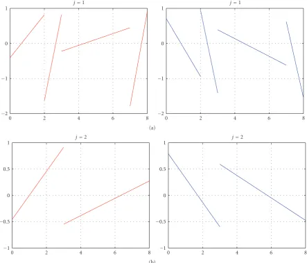
As an example of the previous orthonormalization method,Figure 2presents the linear and quadratic orthonor-mal spline scaling basis functions carried out on the initial finest knot sequence S0 = [τ0d+1 = 0,τ1d+1 = 2,τ2d+1 =
3,τd+1
3 = 7,τ4d+1 = 8]. The left graphs correspond to
the linear case while the right ones correspond to the quadratic case. Three resolution levels are plotted for j =0 (graphs (a)), j = 1 (graphs (b)) and j = 2 (graphs (c)).
Figure 2clearly shows that the constructed scaling functions, at any resolution levelj, are not continuous at the end-points of adjacent intervals of the knots sequenceSj. However, the
continuity feature for many applications is considered as an important characteristic to be satisfied.
The resulting orthonormal wavelet basis developed in [5] is constructed according to the specific traditional multiresolution conditions applied independently on each of the knot sequence’s bounded intervals without imposing any additional condition. The dimension of the wavelet subspace (Wd
j[Ij,i]) on each bounded interval Ij,i is equal to d+ 1.
Figure 3presents an example of the two linear polynomial wavelet functions at resolution levels j=1 (graphs (a)) and
j = 2 (graphs (b)), on the preceding finest sequence S0.
Step 1: transformations Step 2: orthogonalization Spline basis
Bdk,Ij,i(t) k=0,. . .,d ∀i∈N,∀j∈N
Shifting parameters
sd k,Ij,i
Weighting parameters
md k,Ij,i
bdk,Ij,i
bdk,Ij,i
sd k,Ij,i
bdk,Ij,i
bdk,Ij,i
Gram-Shmidt algorithm initial components: bd0,Ij,i,b
d d,Ij,i,b
d d/2,Ij,i
Normalization factors on the global sequenceNd
j,k
Computation of weighting parametersmdk,Ij,i Step 3: continuity Step 4: normalization
Orthonormal piecewise polynomial scaling basis ϕd
j,k(t) k=0,. . .,d;∀j∈N
Figure4: Global orthonormalization scheme.
3. Piecewise Polynomial Scaling Basis Using
New Orthonormalization Procedure
The lack of continuity, as shown in the previous section, is clearly a drawback in many applications. Indeed the approximation error may increase particularly at the points where the fonction presents discontinuities. In some cases, this situation can influence application performances. This section proposes a unified construction of the orthonormal basis of the basic scaling space Vd
0 in such a way that the
functions of the basis are continuous at the end-points of consecutive intervals.
In this paper, the orthonormalization procedure strategy is mainly based on the introduction of additional freedom parameters (named shifting and weighting parameters) on which the procedure controls the partial orthogonality and the continuity of the scaling functions at each end-point of their definition domain. A gradual orthonormalization procedure is proposed where the main steps are summarized by the global scheme inFigure 4.
The procedure is divided into four main parts (see
Figure 4). The first one corresponds to pre-processing trans-formations applied to the spline elements, the second one considers the transformed spline basis orthogonalization problem, the third one deals with continuity and the last one is concerned with the normalization. In order for the presentation to be as general as possible, the basis is directly constructed for any scaling subspace Vd
j, based on the
property that the scaling subspaces are nested (see (13)).
3.1. First Step: Transformations Using Shifting and Weighting Parameters. Rather than working directly on the initial elements of the spline basis, as suggested in [20], we propose a pre-processing step. This step is a partial orthogonalization procedure which ensures two by two orthogonality and the continuity of the extreme and central transformed B-spline functions. This strategy is based on the remark pointed out inSection 2that the spline basis functions are symmetrical by pair, except for one B-spline if the degree of the piecewise
polynomial is even (see Figure 1and (9)). In this context, one can imagine a large family of transformations preserving the property of a basis. However, in this paper the choice is guided by transformations which (i) maintain the initial shapes of the spline elements, and (ii) reduce the number of parameters (controlling the continuity) to be updated during the multiresolution analysis. Trying to be in accordance with points (i) and (ii), we propose the following transformations. The initial B-splines are transformed by shifting parameters ({sd
k,Ij,i}) and weighting parameters ({m d
k,Ij,i}) as described
above.
3.1.1. Shifting Parameters. Each of thed+ 1 initial nonuni-form B-spline functions {Bdk,Ij,i(t)} of (7) follows shift
transformations provided by (16), (17) and (18):
bd
k,Ij,i(t)=s d k,Ij,i+B
d
k,Ij,i(t) fork=0, k=d, (16)
bd
k,Ij,i(t)=s d k,Ij,i+B
d
k,Ij,i(t), b d−k
k,Ij,i(t)= −s d k,Ij,i+B
d−k k,Ij,i(t)
fork=1,. . .,
(d−1) 2
,
(17)
where·is the floor function. Moreover, when dis even, one additional transformation is applied as follows:
bd
k,Ij,i(t)=s d k,Ij,i+B
d
k,Ij,i(t), fork=
d
2. (18)
In the first step, the shifting parameters are computed in order to ensure, in each bounded interval of the knot sequenceSj, the orthogonality conditions between
(i) all functions of (16) and (18):
bd0,Ij,i(t),b d d/2,Ij,i(t)
=0; bd0,Ij,i(t),b d d,Ij,i(t)
=0,
bdd,Ij,i(t),b d d/2,Ij,i(t)
j=0,d=1
(a) −0.5
0 0.5 1
0 1 2 3 4 5 6 7 8
j=1,d=1
(b) −0.5
0 0.5 1
0 1 2 3 4 5 6 7 8
j=2,d=1
(c) −0.5
0 0.5 1
0 1 2 3 4 5 6 7 8
j=0,d=2
(a) −1
−0.5 0 0.5
0 1 2 3 4 5 6 7 8
j=1,d=2
(b) −1
−0.5 0 0.5
0 1 2 3 4 5 6 7 8
j=2,d=2
(c) −1
−0.5 0 0.5
0 1 2 3 4 5 6 7 8
j=0,d=3
(a) −1
0 1 2
0 1 2 3 4 5 6 7 8
j=1,d=3
(b) −1
0 1 2
0 1 2 3 4 5 6 7 8
j=2,d=3
(c) −1
0 1 2
0 1 2 3 4 5 6 7 8
j=0,d=4
(a) −2
−1 0 1
0 1 2 3 4 5 6 7 8
j=1,d=4
(b) −2
−1 0 1
0 1 2 3 4 5 6 7 8
j=2,d=4
(c) −2
−1 0 1
0 1 2 3 4 5 6 7 8
Figure5: Orthonormal scaling spline bases at resolution levelsj=0, 1, 2 from top to bottomd =1 (top left graphs),d =2 (top right graphs)d=3 (bottom left graphs), andd=4 (bottom right graphs) on the finest sequenceS0=[0, 2, 3, 7, 8].
(ii) the two symmetrical functions given by (17) resulting in
bdk,Ij,i(t),b d d−k,Ij,i(t)
=δk(d−k)
fork=1,. . .,
d−1
2
∀i,j∈N,
(20)
where·,·represents the inner product.
It is easy to prove that conditions (19) impose the subsequent relation sd0,Ij,i = s
d
d,Ij,i. Moreover, these values
are independent of the intervals leading therefore to the following equalitysd
0=sdd.
The resolution of the system of equations provided by the second conditions (20) shows that each shifting parameter associated to the corresponding transformed B-spline function is also the same constant value on each bounded interval. So, the shifting parameters are renamed as follows:
sd k,Ij,i=s
d
k fork=0,. . .,
d
2
j=1
−0.15 −0.1 −0.05 0 0.05 0.1
(a)
0 1 2 3 4 5 6 7 8
j=2
−0.4 −0.2 0 0.2 0.4
(b)
0 1 2 3 4 5 6 7 8
j=1
−10 −5 0 5 10 15
(a)
0 1 2 3 4 5 6 7 8
j=2
−0.5 0 0.5 1
(b)
0 1 2 3 4 5 6 7 8
j=1
−1 0 1 2
(a)
0 1 2 3 4 5 6 7 8
j=2
−1.5 −1 −0.5 0 0.5 1
(b)
0 1 2 3 4 5 6 7 8
Figure6: Normalized linear (left graphs) and quadratic (middle and right graphs) spline wavelet functions atj=1, 2.
3.1.2. Weighting Parameters. For the second transformation, we introduce some weighting parameters (mdk,Ij,i) as freedom
parameters in the transformed B-spline functions given by (17) to control the continuity of the new orthogonal functions at the end-points of adjacent intervals (in step 4). The transformed spline functions are given as follows:
bk,Ij,i(t)=s d
k+mdk,Ij,iB d k,Ij,i(t);
bd−k,Ij,i(t)= −s d
k+mdd−k,Ij,iB d d−k,Ij,i(t)
fork=1,. . .,
(d−1) 2
.
(22)
The particular transformed B-spline functions, given by (16) (i.e., the extreme and central (if d is even) ones), do not require weighting parameters. Indeed they naturally ensure the continuity conditions with their neighbors. According to
the particular values of the B-spline functions at the end-points of their definition domain (seeFigure 1), the func-tionsbd0,Ij,i(t),b
d
d,Ij,i(t) andb d
d/2,Ij,i(t) (ifdis even), evaluated
at the end-points of two consecutive intervalsIj,i andIj,i+1
are given by the following relations:
bd0,Ij,i(t2ji)=b d d,Ij,i
t2j(i+1)
=bd0,Ij,i+1
t2j(i+1)
=sd
0+ 1;
bd0,Ij,i
t2j(i+1)
=bdd,Ij,i(t2ji)=b d d,Ij,i+1
t2j(i+1)
=sd
0,
bdd/2,Ij,i(t2ji)=b d d/2,Ij,i
t2j(i+1)
=bdd/2,Ij,i+1
t2j(i+1)
=sdd/2
ifdis even ∀i,j∈N.
(23)
From these equations, we deduce that the continuity of the functions at common end-points of adjacent intervals is naturally satisfied if we swap between the functionsbd
0 1 2 3 4 5 6 7 8 −1
−0.5 0 0.5 1 1.5 2
(a)
−1 −0.5 0 0.5 1
−1 −0.5 0 0.5 1 1.5 2
(b)
−1 −0.5 0 0.5 1
−1 −0.5 0 0.5 1 1.5 2
(c)
−1 −0.5 0 0.5 1
−2 −1.5 −1 −0.5 0 0.5 1 1.5 2
(d)
Figure7: Normalized quadratic spline wavelet functions at resolution levelj=1 satisfying the following conditions: (i) regularityC0with six vanishing moments (a); (ii) regularityC1in the interval [−1, 1] with four vanishing moments (b); (iii) regularityC0in the interval with four vanishing moments (c); (iv) regularityC1in the interval [−1, 1] with three vanishing moments (d).
Decomposition Reconstruction
2
2
2
2
2
2
2
2
Cj−1
Hj−1
Gj−1
Cj Cj
Hj
Gj
Cj+1
Dj+1
H−1j
G−1j
H−1j−1
G−1j−1
Dj
Cj−1
Knots
0 50 100 150 200 250 300 350 400 450 500
Or
ig
inal
sig
nal
0 0.5 1 1.5 2 2.5 3 3.5 4
Figure9: Original discrete signal irregularly spaced “o”.
and bdd,Ij,i(t) and from one interval to another. As for the
functionbdd/2,Ij,i(t) (ifdis even), it is clear that the continuity
is naturally ensured on consecutive intervals. The first two or three (according to the parity of d) elements of the orthogonal basis (see (16)) are now renamed for writing convenience reasons as follows:
bd0,Ij,i(t)=b d
0,Ij,i(t); b d
d/2,Ij,i(t)=b d d/2,Ij,i(t);
bdd,Ij,i(t)=b d
d,Ij,i(t) ifdis even, ∀i,j∈N
bd0,Ij,i(t)=b d
0,Ij,i(t); b d
d,Ij,i(t)=b d d,Ij,i(t)
ifdis odd ∀i,j∈N.
(24)
3.2. Second Step: Global Orthogonalization. The second step takes care of the other orthogonality conditions. We use the classical Gram Schmidt algorithm to supplement the orthogonalization of the piecewise polynomial basis on each bounded interval. The extreme (bd0,Ij,i(t), b
d
d,Ij,i(t)) and or
the central (bdd/2,Ij,i(t)) functions according to the parity of
d, already satisfying the orthogonal conditions are chosen as reference components for the Gram Schmidt orthogo-nalization algorithm. Using the remaining parameterized functions given by (22), the Gram Schmidt method thus complements the construction of the orthogonal scaling basis in a traditional way. The resulting functions are denoted
bdk,Ij,i(t). They are obviously orthogonal and parameterized
by the weighting factorsmdk,Ij,i introduced earlier which are
computed in the following step.
3.3. Third Step: Continuity between Adjacent Intervals. Step 3 is interested in the continuity of other functions of the orthogonal basis (bdk,Ij,i(t) fork = 1,. . .,(d−1)/2)than
those given by (24). The weighting parameters, introduced in step 1, are computed in order to guarantee the continuity
Table1: Shifting and weighting parameters
d Shifting parameters Weighting parameters
1 s1
0= −0.78 not required 2 s2
0= −0.612,s20= −0.373 not required 3 s3
0= −0.485,s30= −0.253 m13=1.925,m32=5.07 4s4
0= −0.395,s40= −0.282,m40= −0.159 m41=0.21,m42=0.594
of each function bdk,Ij,i(t) at the common end-points of
adjacent intervals. For this purpose, we impose the following conditions:
bdk,Ij,i(t2ji)=b d d−k,Ij,i+1
t2j(i+1)
fork=1,. . .,
(d−1) 2
∀i,j∈N.
(25)
For a given spline function degree, the resolution of the sys-tem of equations provided by (25) shows that the weighting parameters are independent of the intervals whatever the resolution levelj, leading to the following relation:
md k,Ij,i=m
d
k fork=1,. . .,
(d−1)
2
∀i,j∈N. (26)
Table 1 provides the shifting and weighting parameters retained for the orthogonal piecewise polynomial scaling basis for different spline function degreesd=1, 2, 3, 4.
3.4. Fourth Step: Normalization Factors. The main objective of the normalization step is to conserve the global finite energy (in L2(R) norm) of the original signal at each
resolution level. In order to preserve the continuity of the scaling functions (bdk,Ij,i, in step 3), we propose to replace
the local factor normalizations performed on each bounded interval with a global factor normalizationNdj,k, computed
on the global sequenceSj=
N−1
i=0 Ij,iat each resolution level j, as follows:
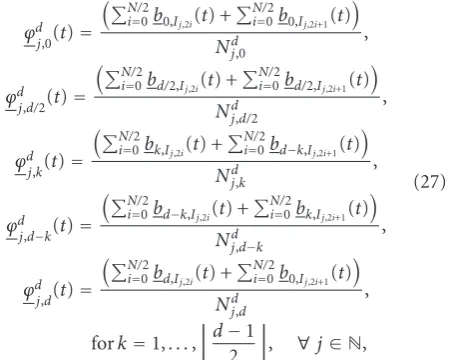
ϕd j,0(t)=
N/2
i=0b0,Ij,2i(t) +
N/2
i=0b0,Ij,2i+1(t)
Nd j,0
,
ϕd j,d/2(t)=
N/2
i=0bd/2,Ij,2i(t) +
N/2
i=0bd/2,Ij,2i+1(t)
Ndj,d/2
,
ϕd j,k(t)=
N/2
i=0bk,Ij,2i(t) +
N/2
i=0bd−k,Ij,2i+1(t)
Ndj,k
,
ϕd
j,d−k(t)=
N/2
i=0bd−k,Ij,2i(t) +
N/2
i=0bk,Ij,2i+1(t)
Nd j,d−k
,
ϕd j,d(t)=
N/2
i=0bd,Ij,2i(t) +
N/2
i=0b0,Ij,2i+1(t)
Ndj,d
,
fork=1,. . .,
d−1
2
, ∀j∈N,
(27)
where ϕd
j,k(t) is the kth global normalized piecewise
Spline degreed=1
0 50 100 150 200 250 300 350 400 450 500
A
ppr
o
ximations
−1 0 1 2 3 4 5
j=1
(a)
Spline degreed=2
0 100 200 300 400 500
A
ppr
o
ximations
−1 0 1 2 3 4 5
j=1
(b)
0 50 100 150 200 250 300 350 400 450 500
Details
−3 −2 −1 0 1 2 3
j=1
(c)
0 100 200 300 400 500
Details
−3 −2 −1 0 1 2 3
j=1
(d)
0 50 100 150 200 250 300 350 400 450 500
A
ppr
o
ximations
−1 0 1 2 3 4 5
j=2
(e)
0 100 200 300 400 500
A
ppr
o
ximations
−1 0 1 2 3 4 5
j=2
(f)
0 100 200 300 400 500
Details
−3 −2 −1 0 1 2 3
j=2
(g)
0 100 200 300 400 500
Details
−3 −2 −1 0 1 2 3
j=2
(h)
piecewise polynomial scaling space, whatever the degree of the spline function, is represented as
Vd
0=
⎧ ⎨
⎩f :f(t)=
d
k=0 ckϕd
0,k(t) fort∈S0 ∀ck∈l2
⎫ ⎬ ⎭.
(28)
For convenience, the normalized basis functions are renamed asBdk,Ij,i(t)=b
d
k,Ij,i(t)/nj,kwhere the new
orthonor-malization factorsnj,kare introduced according to the parity
indexiof the bounded intervalIj,ias follows:
ifiis even:ni
j,k=Nj,k;
ifiis odd:nij,0=Nj,d;nij,k=Nj,d−k,nij,d−k=Nj,kand ni
j,d=Nj,0fork=1,. . .,(d−1)/2.
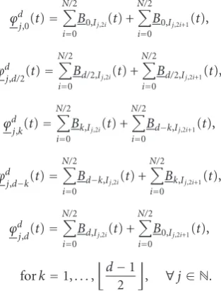
The orthonormal piecewise polynomial scaling basis is thus represented by
ϕdj,0(t)=
N/2
i=0
B0,Ij,2i(t) + N/2
i=0
B0,Ij,2i+1(t),
ϕd j,d/2(t)=
N/2
i=0
Bd/2,Ij,2i(t) + N/2
i=0
Bd/2,Ij,2i+1(t),
ϕd j,k(t)=
N/2
i=0
Bk,Ij,2i(t) + N/2
i=0
Bd−k,Ij,2i+1(t),
ϕd
j,d−k(t)= N/2
i=0
Bd−k,Ij,2i(t) + N/2
i=0
Bk,Ij,2i+1(t),
ϕdj,d(t)=
N/2
i=0
Bd,Ij,2i(t) + N/2
i=0
B0,Ij,2i+1(t),
fork=1,. . .,
d−1
2
, ∀j∈N.
(29)
Based on this new basis orthonormalization procedure,
Figure 5 presents four examples (d = 1, 2, 3, 4) of the orthonormal spline scaling bases of the respective spacesVd
0,
Vd
1 andVd2 for the shifting and weighting parameters given
inTable 1. The layouts are based on this finest knot sequence
S0 =[τ0d+1 =0,τ1d+1 =2,τ2d+1 =3,τ3d+1 =7,τ4d+1 =8]. The
top right graphs ofFigure 5present the continuous quadratic piecewise polynomial scaling functions. The dashed lines, on each resolution levels (graphs (a), (b), (c)), correspond to the functionϕ2
j,1(t). The solid lines are concerned with the
func-tionϕ2
j,1(t) at each resolution level. Finally, the marked lines
(+) represent the function ϕ2
j,0(t) at each resolution level.
The proposed scaling functions are continuous everywhere. The regularity of the scaling functions is of order zero at all joining intervals. This is inherent to the multiplicity which has been imposed on each knot of the considered sequence (see (5)).
4. Piecewise Polynomial Wavelet Basis Using
New Orthonormalization Procedure
The following section is devoted to a unified orthonor-mal piecewise polynomial wavelet basis construction of the detail subspace whatever the degree of the spline function. Due to the multiplicity of the knots, we are going to show in the following pages that one can work with a single wavelet. Moreover, the continuity of the wavelet function being ensured again by relaxing the tra-ditional normalization procedure (i.e., going to a normal-ization on each interval to a normalnormal-ization on the global sequence).
4.1. Piecewise Polynomial Wavelet Subspace Dimension. Let us consider two consecutive intervals Ij−1,i
Ij−1,i+1 at
resolution level j −1. As seen in Section 2, the scaling and wavelet subspaces are linked by (14). The piecewise polynomial scaling subspace Vd
0[I0,i]
Vd
0[I0,i+1] contains
Wd
1[I1,i]. Therefore, any wavelet functionψkd,I1,i(t)∈W d 1[I1,i]
defined on the bounded interval I1,i can be
decom-posed using the orthonormal basis of the scaling subspace
Vd
0[I0,i]
Vd
0[I0,i+1] as follows:
ψkd,I1,i(t)= 2i+1
m=2i d
n=0
g1,mk,nBdn,I0,i(t) ∀i,k∈N. (30)
This wavelet function is parameterized by 2(d+ 1) coeffi -cients, denoted{g1,mk,n}, which must be computed.
As the multiplicity μof the knot to remove (τd+1 2j−1(i+1))
decreases, the dimension of the piecewise polynomial scaling subspace, restricted to any intervalIj−1,i
Ij−1,i+1, decreases
progressively leading to the nested scaling subspaces:
Vd
j−1
τ2dj+1−1i,τ2d+1j−1(i+1) Vdj−1
τ2d+1j−1(i+1),τ2dj+1−1(i+2)
⊃Vd j−1
τd+1
2j−1i,τ2dj−1(i+1),τ2dj+1−1(i+2)
⊃ · · · ⊃Vd j−1
τ2dj+1−1i,τ21j−1(i+1),τ2d+1j−1(i+2)
⊃Vd j−1
τd+1
2j−1i,τ2dj+1−1(i+2)
∀i∈N, j≥1.
(31)
According to (14), the piecewise polynomial wavelet subspace dimension, restricted toIj,i, is deduced as follows:
dimWd j
Ij,i
=dimVd j−1
Ij−1,i Vdj−1
Ij−1,i+1
−dimVd j
Ij,i
,
(32)
where the dimension of the scaling subspace (dim(Vd j[τ2d+1ji ,
(31), the dimension of the scaling subspace at resolution level
j−1 is given as follows:
dimVd j−1
τ2dj+1−1i,τ21j−1(i+1),τ2dj+1−1(i+2)
≤dimVd j−1
Ij−1,i Vdj−1
Ij−1,i+1
≤dimVd j−1
τ2dj+1−1(i+1),τ2dj+1−1(i+2)
Vd
j−1
τd+1
2j−1(i+1),τ2dj+1−1(i+2)
∀i∈N,j≥1.
(33)
Then it translates into
d+ 2≤dimVd
j−1
Ij−1,i Vdj−1
Ij−1,i+1
≤2(d+ 1) ∀i∈N, ∀j≥1.
(34)
According to (32) and (34), we deduce that the dimen-sion of the wavelet subspace, restricted toIj,i, lies between
one andd+ 1:
1≤dimWd j
Ij,i
≤d+ 1 ∀i∈N, ∀j≥1. (35)
This last equation means that we have the possibility of choosing several wavelet bases of various dimensions. Remember that the wavelet functionψd
k,I1,i(t) is
parameter-ized by 2(d+ 1) coefficients{g1,mk,n} (see (30)). In order to
minimize the computational cost due to these coefficients, the smallest subspace dimension is retained. In theory, this choice requires to process the scaling subspace of dimension
d+ 2 at resolution level j −1. However, it is easy to note that the approximated signal at the knotτ2μj−1(i+1)(with 1 ≤
μ ≤ d+ 1) in any piecewise polynomial scaling subspaces at resolution level j−1 is the same value due to the chosen interpolation method used in this paper. Hence the quality of the detail signal at the knotτ2μj−1(i+1)(with 1≤μ≤d+ 1)
is not affected by any particular selected scaling subspace dimension.
For computational simplicity, we choose the scaling subspaces of dimension 2(d+1) rather thand+2. The scaling functions belonging to the subspace of dimension 2(d+ 1) are easily computed since generalization formulas have been provided in [19]. Thus, at any resolution level j, equation (30) becomes
ψd 1,Ij,i(t)=
2i+1
m=2i d
n=0
gmj,1,nBdn,Ij,i(t) ∀i∈N, ∀j≥1. (36)
4.2. Computation of the Wavelet Coefficients Using Traditional Conditions. The wavelet function (see (36)) requires the computation of 2(d+ 1) unknown coefficients{gmj,1,n}. For
this purpose, we impose two sets of conditions. The first nec-essary set is directly related to the traditional multiresolution concept. On each interval of the knot sequence the wavelet subspace must be as follows:
(i) orthogonal to the scaling subspace, at any resolution level (j≥1) resulting in
ψd
1,Ij,i(t),B d k,Ij,i(t)
=0 fork=0,. . ., ∀i∈N, ∀j≥1 (37)
(ii) orthogonal to the wavelet subspaces at all and cross scales, resulting in
ψd
1,Ij,i(t),ψ d 1,Ik,p(t)
=αδjkδip ∀i,p∈N, ∀j,k≥1, (38)
where α is a multiplicative constant; δpq is the Kronecker
symbol which is equal to 1 ifp=qand to 0 ifp /=q. Since conditions (37) and (38) do not fully determine 2(d+ 1) unknown coefficients{gmj,1,n}, we introduce a second
category of conditions. This category is concerned with additional useful conditions imposed on the wavelet so that the function satisfies the most significant desirable features often required for a “good” wavelet function (continuity, even differentiability, vanishing moments).
4.3. Computation of the Wavelet Coefficients Using Additional Conditions. These additional conditions have been studied extensively. We propose to establish condition priorities gathered in different classes depending on the degree of the spline function.
4.3.1. Continuity inside the Interval. In this category, we start with the first class of requirements ensuring theC0wavelet
function regularity inside each intervalIj,iat the particular
knott2j−1(i+1)as follows: d
n=0
g2j,1i,nBdn,Ij−1,i
t2j−1(i+1)
=
d
n=0
g2j,1i+1,nBdn,Ij−1,i
t2j−1(i+1)
∀i,k∈N,∀j≥1.
(39)
If the number of unknown coefficients{g1,mk,n} for a given
degree d is less than the number of requirements, more conditions are necessary as described below.
4.3.2. Continuity at the Boundary Points of Consecutive Interval. The second class of conditions proposes to follow the C0 regularity of the wavelet functions now on the
global sequence Sj at any resolution level j. In order to
impose the continuity of the wavelets between different end-points of consecutive intervals, we suggest keeping one specific coefficient among the different coefficients {gmj,1,n}
to guarantee the link between two consecutive intervals Ij,i
andIj,i+1. The selected coefficient in the intervalIj,i+1is then
related to the selected coefficient in the preceding intervalIj,i
using the relationship deduced from the following equation:
ψ1,dIj,i
t2j(i+1)
=ψ1,dIj,i+1
t2j(i+1)
∀i∈N, ∀j≥1. (40)
When going from one interval to the adjacent one, the selected coefficient (e.g.,gmj,1,n with 0≤ n ≤ d) inIj,i+1 is
then updated. If the number of unknown coefficients{g1,mk,n}
for a given degreedis less than the number of requirements, more conditions are necessary as follows.
with the shape of the wavelet on any bounded intervalIj,i.
One can choose one among the four conditions to control the number of vanishing moments according to the desired shape of the wavelet function as given below:
ψd 1,Ij,i(t2ji)
= ⎧ ⎪ ⎨ ⎪ ⎩
±ψ1,dIj,i
t2j(i+1)
∀i∈N,∀j≥1,
ψ1,dIj,i
t2j(i+1)
±ψ1,dIj,i
t2j−1(i+1)
∀i∈N,∀j≥1.
(41)
Once again if the number of unknown coefficients{g1,mk,n}for
a given degreed is less than the number of requirements, more conditions are necessary as described below.
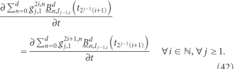
4.3.4. Continuity of the First Derivative inside the Interval. The fourth class of conditions guarantees the C1 wavelet
function regularity inside any interval Ij,i. The continuity
conditions of the first derivative of the wavelet function, at the particular knott2j−1(i+1) inside any intervalIj,iin which
the function belongs results in
∂dn=0g 2i,n j,1Bdn,Ij−1,i
t2j−1(i+1)
∂t
=∂ d
n=0g2j,1i+1,nBdn,Ij−1,i
t2j−1(i+1)
∂t ∀i∈N,∀j≥1.
(42)
We keep increasing the list of conditions until reaching the maximum number of conditions, that is, 2(d+ 1). In this basis orthonormalization procedure we have chosen to ensure primarily the continuity of all achievable derivatives of the wavelet function at the particular pointt2j−1(i+1)inside
the interval Ij,i. Then we complete with the derivatives
continuity conditions of the function at the end-points ofIj,i
if necessary.
4.3.5. Normalization on the Global Sequence. To preserve the
C0regularity of the wavelet function as described previously,
a global normalization factor is applied to the complete sequenceSj. Remember that one coefficient (e.g.,gm,n
j,1 with
0≤n≤d) is used to ensure theC0wavelet regularity onS j.
The initial value of the coefficientg0,j,1n (in the first interval Ij,0) is computed in such a way that the wavelet function is
globally normalized onSjonce for all.
4.3.6. Discussions. As seen above, a large family of piecewise polynomial wavelet basis can thus be constructed. But these wavelets are not all used to implement the multiresolution approach since they generate stability problems depending on a particular configuration of the knots in the sequence. Particular attention concerning the wavelet stability must be given when constructed. The stability problem occurs when the waveletψd
1,Ij,i(t) evaluated at the knott2j−1(i+1) inside the
intervalIj,i or at the end-pointt2j(i+1) of the same interval
is equal to zero. If the wavelet function is equal to zero at
the pointt2j(i+1), the chosen parametergm,n
j,1 is automatically
equal to zero therefore leading to wavelet functionsψ1,dIj,i(t)
which are null on each interval of the considered sequence (see (40)). To overcome the stability problems, the wavelet function must meet the following requirements:
ψ1,dIj−1,i(t)=/0, ψ d
1,Ij−1,i(t)=/ 0, g m,n
j,1 =/0 ∀j≥1. (43)
The wavelet, denoted byψdj(t), of the detail subspaceWdj is
now deduced as follows:
ψdj(t)= N−1
i=0
ψ1,dIj,i(t) ∀j≥1. (44)
With this wavelet basis orthonormalization procedure, the wavelet regularity inside the interval is Cd−1 for d > 2.
Increasing the spline function degree allows us to ensure the wavelet derivatives continuity everywhere.
Figure 6presents the linear (left graphs) and quadratic (middle and right graphs with different relationships at the boundary points) piecewise polynomial wavelet at two resolution levels j = 1 (graph (a)) and j = 2 (graph (b)) constructed on the previous finest initial knot sequence:
S0 =[0, 2, 3, 7, 8]. The number of wavelet functions initially
equal to two for d = 1 and three for d = 2, as described inSection 2.3, is reduced to only one function on each bounded interval. Moreover, the quadratic wavelet is continuous inside the bounded interval (regularityC0) and
at the end-point of adjacent intervals. It is possible to increase the regularity of the quadratic wavelet inside each bounded interval if the condition (41) is replaced by the continuity condition of the wavelet first derivatives at the point inside the considered interval. Examples are given by the second and fourth graphs of Figure 7where the continuity of the quadratic wavelet first derivative at the point 0 is ensured. Rather than satisfying the condition given by (40), one can increase the number of vanishing moments of the wavelet such as illustrated by the first graph ofFigure 7. However, conditions (41) are useful for decomposing any discret signal regularly sampled. Although the wavelet basis is orthogonal, the proposed wavelet becomes symmetric and compactly supported (see the graphs (b), (c) and (d) ofFigure 7).
5. Orthogonal Decomposition Algorithm
This section is concerned with the orthogonal decompo-sition of a signal y(t) represented by its discrete samples irregularly spaced y(ti). We assume that this signal lives in
the basic spline spaceVd
0. The approximation of the signal y(t) at resolution level j, on each bounded interval Ij,i,
is denoted yIj,i(t). This signal belongs to the scaling space
Vjd[Ij,i]. As seen earlier, the piecewise polynomial scaling and
wavelet subspaces satisfy the orthogonal property given by (14). Therefore, one can decompose any signal yIj−1,i(t) +
yIj−1,i+1(t) ∈ V d
j−1[Ij−1,i]
Vdj−1[Ij−1,i+1], according to the
relation
yIj−1,2i(t) +yIj−1,2i+1(t)=yIj,i(t) +rIj,i(t) ∀i∈N,∀j≥1,