Górka, Tomasz (2009): Methodical Research and Further Development of Caesium Magnetometry for the Investigation of Geoglyphs of Palpa/Nasca, Southern Peru. Dissertation, LMU München: Fakultät für Geowissenschaften

(1)

M

ETHODICAL

R

ESEARCH

AND

F

URTHER

D

EVELOPMENT

OF

C

AESIUM

M

AGNETOMETRY

FOR

THE

I

NVESTIGATION

OF

G

EOGLYPHS

OF

P

ALPA

/N

ASCA

, S

OUTHERN

P

ERU

Dissertation

zur Erlangung des Doktorgrades der Fakultät für Geowissenschaften der Ludwig – Maximilians – Universität München

vorgelegt von

Tomasz Górka

(2)

Erster Berichterstatter: Prof. Dr. Valerian Bachtadse Zweiter Berichterstatter: Prof. Dr. Heinrich C. Soffel

(3)

(4)

Abstract

Page I

Abstract

The geoglyphs of Palpa and Nasca in southern Peru have been considered one of

the greatest mysteries of archaeology (Aveni 1990). Thousands of lines, cleared fields and

figures were carved on flat plateaus in the desert, the so called pampas, during the Paracas

and Nasca cultures (800 BC 650 AD). The geoglyphs of Palpa have been studied in detail

with archaeological methods since 1997 by the Nasca Palpa Project (Reindel and Grün

2006). In the framework of this project, the first prospection with geophysical methods in

the pampa was conducted in 2003 (Fassbinder and Reindel 2005). During the following

field seasons five geoglyph sites in the vicinity of Palpa were chosen that had previously

been documented through a combined field survey and analysis of high resolution aerial

images (Lambers 2006). Since the geoglyphs of Palpa and Nasca have been declared the

UNESCO World Heritage, the best non destructive technique of site exploration to detect

and map possible features beneath the trapezoids, turned to be the magnetic prospecting.

So far, magnetometry has rarely been used for archaeological surveying in South

America. As the magnetic inclination in Palpa is less than 3° and the intensity of the total

Earth’s magnetic field hardly exceeds 25.000 Nanotesla, the highly sensitive total field

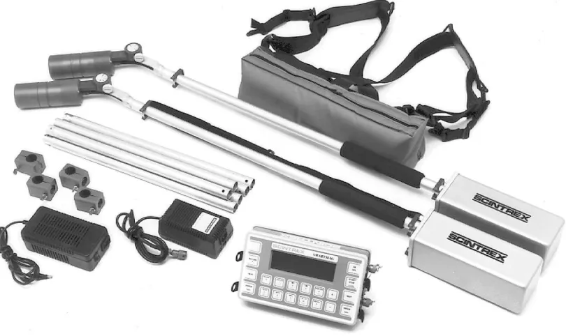
caesium magnetometer (Scintrex SmartMag SM4G Special), to be used during fieldwork,

needed to be adapted to these conditions. In addition, geochemical processes forming iron

oxides in soil, which usually cause clear magnetic anomalies, could not be expected there

because of the lack of precipitation. On the contrary, due to the shallow inclination of the

Earth’s magnetic field, simple anomalies created more complicated patterns, which were

difficult to interpret. To overcome this problem and to enhance the visibility of magnetic

data, two sensors were arranged in a horizontal gradiometer configuration. The application

of the magnetometer in such an arrangement, in combination with magnetic total field data,

(5)

Abstract

Page II equator. This enabled to trace the older geoglyphs that had been obliterated during the

gradual surface clearing carried out on the same sites in Nasca times.

The present study reports on the results of the magnetic prospecting on five large

geoglyph complexes located on the pampas to the north, east, west and south of Palpa.

Most of these places were in use during several centuries and developed in time (Lambers

2006). The sites were enlarged or remodelled, which led to the destruction of older lines by

the trapezoids. During their construction the stones between the existing lines were

removed, which efficiently wiped out the older lines from the surface. The magnetic images

clearly revealed the course of those lines on all five investigated sites.

It is believed that the older lineal geoglyphs are visible in the magnetograms due to

their heavily compacted surface, which was caused by people frequently walking over them

in the course of ritual activity taking place on geoglyph sites. This compaction destroyed the

vesicular horizon of exposed loess sediments and its remanent magnetization. On the

contrary, the large trapezoids constructed later did not confine movement of people over

them, so their surface is generally less compacted. For this reason, the older lines are visible

in the magnetograms even though their cleared surface resembles that of the trapezoids.

Apart from the geoglyphs, the magnetic measurements showed anomalies that

may be interpreted as traces of buildings, postholes, pits or other man made structures. The

relation of these features to the geoglyphs has been also investigated.

In conclusion, the magnetic surveying not only shed new light on the development

of large geoglyph complexes over time but also on the understanding of the Paracas and

Nasca cultures and the history of the region in general. Without destruction and excavation,

(6)

Contents

Page III

4.1 Magnetic field of the Earth 17 4.2 Magnetic susceptibility and magnetic minerals 18 4.3 Magnetic remanence 20 4.4 Magnetic anomalies on archaeological sites 21 4.5 Soil magnetism on archaeological sites 25 4.5.1 Magnetic enhancement mechanisms 26 4.5.2 Soil magnetism on geoglyph sites 27 4.6 Time variations in the Earth’s magnetic field 28 Chapter 5 Methodology ……….. 30

5.1 Instrumentation and sampling procedure 30 5.2 Data acquisition and processing 35 5.3 Presentation and interpretation of results 39 5.3.1 Presentation of results 39 5.3.2 Interpretation of results 40 5.4 Common laboratory procedures in this work 42 Chapter 6 Results of geophysical prospecting on site PP01 36 “Llipata” ………. 43

Chapter 7 Results of geophysical prospecting on site PV67A 15/16 “Yunama” ………. 56

Chapter 8 Results of geophysical prospecting on site PV67A 47 “Sacramento” ………. 69

Chapter 9 Results of geophysical prospecting on site PV67B 55 “Carapo” ……… 86

Chapter 10 Results of geophysical prospecting on site PP01 49 “San Ignacio”……….. 96

Chapter 11 Synopsis ……… 104

Chapter 12 Last Word and Conclusions ………. 107

References ……… 109

List of figures ……….. 117

List of tables ……… 123

Acknowledgments ……….. 124

(7)

(8)

Chapter 1 – Introduction

Page 1

Chapter 1 Introduction

1.1. PREFACE

Magnetic investigations have long been a source of productive interaction between

archaeology and geophysics (Aitken 1974). Together with resistivity survey they are one of

the earliest applications of geophysical prospecting and are nowadays well established as a

standard method for archaeology (Linington 1970). Although numerous techniques of

geophysical surveying have been applied to site exploration, it was magnetometry that

happened to be the most important way in which physics has been involved in

archaeological research. Such fusion formed a new scientific area, which essentially grew

out of the numerous interdisciplinary studies involving highly sophisticated technical

methods for detecting and mapping otherwise not accessible archaeological features. This

relatively new science, frequently termed as

archaeological prospecting

, has well developed into a separate scientific discipline with its own specialities, in which almost all the

techniques were initially derived from methods used in geological geophysical prospecting

and conventional aerial survey (Scollar et al. 1990). This combination of archaeology, aerial

photography, remote sensing, and geophysics has been accurately described by Anthony

Clark (1990):

(9)

Page 2

1.2. FOREWORD TO THE PROJECT

The geoglyphs of Palpa/Nasca are the geometrical and biomorphic figures drawn

on the desert surface by pre Columbian cultures in Southern Peru (Figure 1.1; compare

Chapter 2). They have been studied in detail with archaeological methods since 1997 by the

Nasca Palpa Project (Reindel and Grün 2006) supported by the Swiss Lichtenstein

Foundation for Archaeological Research Abroad (SLSA) and the German Federal Ministry

of Education and Research (BMBF). In the framework of the sponsoring program “NTG –

New Scientific Methods and Technologies in Humanities”, the first prospecting with

geophysical methods has been conducted in the year 2003 (Fassbinder and Reindel 2005)

as a result of the cooperation between Bavarian State Department of Monument and Sites

(BLfD Munich) and the German Archaeological Institute, Commission for Archaeology of

Non European Cultures (KAAK DAI Bonn).

Figure 1.1 Figure 1.1 Figure 1.1

Figure 1.1. Reloj Solar (Sun Dial) geoglyph complex located on the southern slope of Cresta de Sacramento, north of Palpa; source – DAI: http://www.dainst.org/index_593_de.html

Since the geoglyphs of Palpa and Nasca have been declared a UNESCO World

Heritage site, the geophysical prospecting was the only none destructive technique of site

exploration apart from aerial archaeology, and the main tool to detect and map possible

(10)

Page 3 seasons, in joint effort with BLfD, geophysicists from the Department of Earth and

Environmental Sciences of the Ludwig Maximilian University Munich, have measured

approximately 60 Ha of studied project territory covering entirely five foremost geoglyph

complexes.

1.3. OBJECTIVES AND MAIN TASKS

The general aim of the Nasca – Palpa project was the study of the cultural and

palaeoenvironmental history of the Palpa region on the Peruvian southern coast. By means

of surveying, mapping, excavations and geoarchaeological research, a systematic

documentation of the cultural heritage (among others geoglyphs) was pursued to establish a

basis for scientific investigation of the cultural history. Various survey and dating methods

and technologies were developed, enhanced, as well as tested under different conditions.

Through the applications of these methods, archaeologists and natural scientists cooperated

closely working on the reconstruction of life and environment of the past cultures of the

region (http://www.dainst.org/index_593_de.html on 21.03.2008).

Most of the geoglyph complexes were in use during several centuries and grew

considerably over time, new drawings were frequently added and existing ones enlarged or

remodelled. In this process, large trapezoids often covered older lines. During their

construction the stones of the desert pavement between the existing lines were removed,

making the older lines invisible on the surface. Therefore, the major objective was:

o the detection and interpretation of obliterated archaeological structures

within the trapezoidal figures, in particular the disclosure of the course of

the previous linear patterns.

The enhancement of the magnetic sensitivity of the measuring device in relatively

unfavourable geophysical conditions on Peruvian sites, in addition to the improvement of

the fieldwork methods for further application in Europe, became the main technical aim.

It was based on the identification of the differences in the measurements of the

archaeological anomalies on the example of these two unlike environments. From the

archaeological point of view, the most important reason of geophysical contribution was the

(11)

Page 4 chronology of the Peruvian southern coast. This was coupled with the primary goal of the

project – the preservation of one of the most important South American archaeological

monument complexes.

In order to achieve the given objectives, a number of tasks had to be completed in

due course of the considered research activities. The most important ones are briefly

summarized as follows:

o Improvement of the new magnetometer system for archaeological

prospecting, which implied the further development of the commercial

geophysical device (Scintrex Smartmag SM4G) for data collection in the

field. It was combined with the adjustment of the instrument to the

archaeological applications in the region of geomagnetic inclination close

to the limits of operating zone of the apparatus (2° to 86° based on the

specifications of CS3 sensor, Scintrex, Ltd.).

o Development of new digital image processing techniques for the more

precise and accurate interpretation of magnetic anomalies (for information

on magnetic anomalies see Chapter 4.4).

o Assessment of the specific measurement conditions in Peru (in comparison

to Europe) and resulting dissimilarities in the size and shape of anomalies

due to the shallow inclination of the local geomagnetic field.

o Application of the caesium magnetometer to the geoglyphs and execution

of series of measurements on site, covering most significant complexes in

the vicinity of Palpa, during several annual field campaigns.

o Study of the archaeological setting of Paracas and Nasca cultures and the

geoglyphs background, for the better understanding of archaeological

structures on site and resulting variations in magnetic images.

o Data processing and visualisation work on the collected data set using

series of highly developed computer programs.

o Interpretation by the combination of geophysical results with the

(12)

Chapter 2 – Palpa Geoglyphs and Their Archaeological Setting

Page 5

Chapter 2 Palpa Geoglyphs and Their

Archaeological Setting

The Geoglyphs of Nasca and Palpa in southern Peru have been considered one of

the greatest mysteries of archaeology (Aveni 1990). Over an area of several hundred square

kilometers, on flat plateaus called "pampas", ancient civilizations have carved an array of

over thousand geometrical and biomorphic figures of varying size and precision into the

earth. Lines several kilometers long, rectangles and trapezoids several hectars large, human

figures on hillsides, and huge depictions of animals and plants were drawn on the desert

surface already in prehispanic times during the Paracas and Nasca cultures (800 BC 650

AD) (Grün et al. 2000; Sauerbier and Lambers 2003; Lambers 2006) (Table 2.1).

Unfortunately, the understanding of geoglyphs has been hindered for a long time

by the lack of an accurate documentation (Sauerbier and Lambers 2003). Ever since the

first report in 1927 by Peruvian archaeologist Toribio Mejía Xesspe, serious archaeological

investigations have by far been outnumbered by unscientific interpretations. Additionaly,

the whole Palpa area of the Nasca basin and the geoglyphs located in its close proximity

have been largely ignored by archaeological researchers, although they are comparable in

quality and complexity to the better known ones on the Nasca pampa. There has also been

a lack of public interest in them and little or no protection, although they are part of the

same cultural phenomenon (Lambers 2006). For those reasons as well as for the fact that in

this area geoglyphs are located close to densely settled zones along the valley floors, which

makes it an easier place to study the relationships between two classes of cultural remains

(Lambers 2006), the Palpa region was chosen as the new area of interdisciplinary geoglyph

(13)

Page 6 The Nasca drainage provide many suitable spots to place geoglyphs. It is restricted

by the foothills of the Andes to the northeast and by the coastal mountain range to the

southwest. This unique topographic feature which led to the development of a large basin

and later a vast sediment plain (Chapter 3.3 – Geographical and Geological Setting), proved

to be crucial for the creation of these remarkable drawings.

In order to construct a geoglyph on flat plateaus, darkly oxidized stones of the

natural desert pavement were removed and heaped along the border of the cleared area,

thereby revealing a bright layer of sand and silt standing out in strong contrast to the

surrounding undisturbed surface. Piling the dark stones up at another place considerably

enhanced the contrast in color and brightnest between the original and altered surface

(Lambers 2006).

Figure 2.1 Figure 2.1Figure 2.1

Figure 2.1. Geoglyph complex along the northern edge of the Nasca pampa (black line – Panamerican Highway); source NASA

When geoglyphs were constructed, the underlying sandy deposits were exposed

allowing the silty elements together with humidity to develop a thin crust on top of the layer.

It prevented a wind erosion and permitted the preservation of the geoglyphs. Moreover,

as the Atacama Desert between northern Chile and southern Peru is one of the driest areas

(14)

Page 7 desert floor, thus erosion by water runoff has been rare for centuries. For that reason and

due to the development of the crusty layer, the enigmatic Nasca Lines have survived almost

unaltered and are easily visible today.

The predominant kind of prehispanic geoglyph found on the large flat plateaus is a

cleared area often in trapezoidal or rectangular form (Figure 2.1). It is usually accompanied

by lines running straight or bending several times, forming zig zags, meanders or spirals.

Biomorphic figures constitute the smallest fraction of the whole corpus, but at the same time

they are the most famous designs. A common feature of the geoglyphs is that they occur

together in complexes, often crosscutting each other, with older geoglyphs obliterated by

more recent ones. The new drawings were added to existing ones in such a way that older

geoglyphs were not build over, but rather incorporated into the group. They are therefore

the result of several working steps: lateral enlargements, repeated surface clearing and

redrawing on the same place (Lambers 2006). This makes the older geoglyphs not visible

for majority of the ground archaeological techniques as well as for the aerial imaging. Thus,

a powerful geophysical method had to be applied in order to trace previously obliterated

patterns (see Chapter 5 – Methodology).

Date Period Archaeological culture Phase

1532 AD Late Horizon Inca

1400 AD Late Intermediate Period Ica/Chincha

1000 AD Middle Horizon Wari

600 AD 450 AD 250 AD

Early Intermediate Period Nasca

Late Middle

Early

1 BC Initial Nasca

200 BC 400 BC 600 BC

Early Horizon Paracas

Late Middle

Early

800 BC Initial Period

1800 BC Archaic

Table 2.1 Table 2.1 Table 2.1

Table 2.1. Chronology and the cultural history of the Nasca basin (dates based on preliminary results of the Nasca – Palpa Project); after Lambers (2006).

Although it is commonly assumed that most of these earth drawings have been

produced by the Nasca people that emerged out of the preceding Paracas culture (Table

(15)

Page 8 have been put forward by reputable Nasca researches like: Paul Kosok (1965), Maria Reiche

(1976), Anthony Aveni (1990), Peris Clarkson (1990), Gary Urton (1990), Heleine

Silverman (1990), David Johnson (1990), David Browne (1992), Maria Rostworowski

(1993), Johan Reinhard (1996), Aurelio Rodriquez (1999), as well as by those less

renowned. As a result there exist more than twenty of theories offering explanations. Those

acceptable ones may be classified into the following categories (Aveni 1990):

o Solar, star or moon calendar and astronomy,

o Indicators for underground water, irrigation and agriculture.

o Ceremonial practices, mountain or fertility cult,

o Geometry and artistic expression,

o Movement, communication, transportation.

The variety of different patterns and figures is so large that it is hard to believe that

these drawings did serve just one specific purpose (Aveni 1990). Nevertheless, as the

archaeological excavations uncovered broken pottery and ample evidence of offerings and

sacrifices, including guinea pigs, corn, crayfish and

Spondylus

seashells from thousand kilometres away, it seems that the sites had mainly a religious function (Reindel et al. 2003;

Curry 2007). As some of the project archaeologists declare: “they were locations, not

pictures”.Concerning the chronology of the geoglyphs, they are believed of having been

created in a period of 1000 years (Table 2.1). Over such a long time, cultural change can be

expected to affect their construction, use, perception and physical manifestation. Thus, the

presented theories have to be improved by adding the time depth (Lambers 2006).

The geoglyph chronology from Palpa region relies mainly on the relative datings

using the stratigraphic relationships of specified geoglyphs along with the classification of

associated ceramics, as well as direct chronometric datings obtained using scientific

methods (e.g. optically stimulated luminescence measurements or accelerator mass

spectrometry radiocarbon dating) (Greilich et al. 2004, Kadereit et al. 2007). Available

chronological evidence from Palpa suggests that the earliest geoglyphs date to the Early

Horizon (Table 2.1), although the precise starting date remains unclear. Geoglyph related

activity is in any case present in Late Paracas and increases in Initial Nasca, reaching its

peak in the Early Nasca period. Afterwards it decreases continuously through Middle and

(16)

Page 9 Unfortunately, the most frequent geoglyph types on which geophysical prospecting

was performed, the straight lines and trapezoids, have no chronological relevance since they

cover the whole time span of the geoglyph phenomenon (Lambers 2006). In general,

geoglyph variety was greatest in the Early Nasca period when all kinds of geoglyphs were

made and used. Antropomorphic figures, probably the earliest ones, were typical until Early

Nasca, when spirals, biomorphic figures, and different line types coexisted with trapezoids

and rectangles. Later diversity was reduced to certain line types and areal forms. By Late

Nasca times, only straight and meandering lines and large areal geoglyphs had survived.

Thus, these types were not only common forms throughout all phases of geoglyph creation,

but represented also the standard to which the geoglyph repertoire was finally reduced

(Lambers 2006).

The construction and use of the geoglyphs and their associated structures were not

separated, but were considered as parts of an integrated whole. Many groups of people

were involved in geoglyph related activity over a long period of time. The following kinds of

activity, summarized by Lambers (2006), could be recognized on the geoglyphs of Palpa:

o Construction and remodelling of geoglyphs and stone structures,

o Walking on lineal geoglyphs and around stone structures,

o Placing and breaking of pots on or along borders of lines and trapezoids,

o Placing of vessels, field crops, shells, and other objects on stone structures,

o Erection of wooden posts on trapezoids close to the stone structures,

sometimes accompanied by placing of offerings in the excavated pit.

o Food consumption and placing,

o Cleaning and maintenance of geoglyphs,

o Burying of stone structures at the end of their use.

The precise documentation of these well defined activities related to geoglyphs is

particularly important for the correct understanding of the origin of anomalies measured by

geophysical means. As indicated in due course of this study (see Chapter 4.5), the repetitive

geoglyph walking resulting in heavy compaction of line surfaces, as well as vessel and pot

placing along with erection of wooden posts, could have been the crucial activities for later

(17)

Chapter 3 – Area of Research

Page 10

Chapter 3 Area of Research

3.1. LOCATION

The Palpa and Nasca geoglyphs are located in the Peruvian costal plain, which is

high arid plateau that stretches around 50 km between the towns of Nasca and Palpa on the

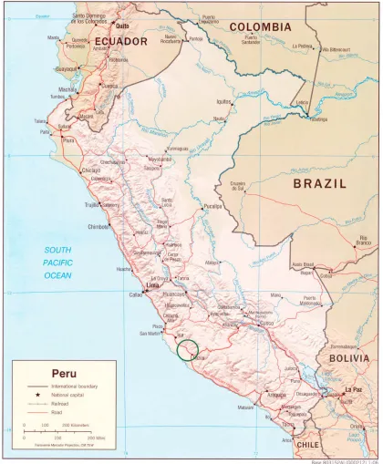
Pampas de Jumana in Peru. The geoglyphs are situated approximately 400 km south of the

capital Lima and cover about 450 km2 of the desert territory (see figures 3.1, 3.2 and 3.3).

Figure 3.1. Map of the Ica Region (Southern Peru) (SLSA Zürich; DAI Bonn)

Figure 3.2.Satellite photograph of the Provinces of Palpa and Nasca (Southern Peru) (SLSA Zürich;

(18)

Page 11 The desert itself occupies a strip along the southern Pacific coast of Peru extending

from the shoreline 20 100 km inland to the secondary ridges of the Andes Mountains.

There, in the Provinces of Palpa and Nasca, the world’s largest concentration of ground

drawings is located. For the purposes presented in Chapter 2, the area of research was

carefully selected in the close surroundings of the city of Palpa (Figure 3.4).

(19)

Page 12 Figure 3.4

Figure 3.4 Figure 3.4

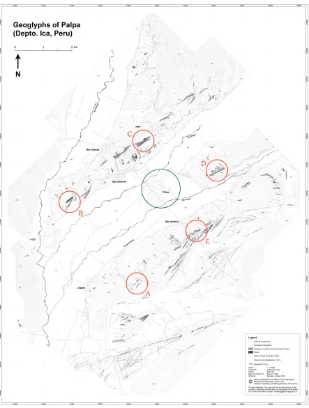
Figure 3.4. Area of research; red circles represent 5 measured geoglyph complexes surrounding the modern city of Palpa (green circle): A – PP01 36 Llipata, B – PV67A 15/16 Yunama, C – PV67A 47 Sacramento, D – PV67B 55 Carapo and E – PP01 49 San Ignacio; source Depto. Ica, Peru; SLSA Zürich, ETH Zürich;

(20)

Page 13 Palpa itself is a modern settlement situated in the broad valley formed by Rio Palpa

and Rio Viscas. Both rivers flow to the southeast until their junction with Rio Grande shortly

thereafter, which is the only waterway of the whole drainage system having its perennial

runoff to the Pacific Ocean. On the slopes and plateaus stretching along the rivers a vast

geoglyph concentration can be found. In the present study a thorough investigation of five

main complexes was made. During the several field campaigns within the years 2003 and

2007, the main geoglyph plateaus, which are presented in chronological order below, were

covered by means of geophysical prospecting (see Figure 3.4 and Table 3.1):

o

PP01 36

(PAP379) located on Pampa de Llipata (to the south of Palpa), o

PV67A 15/16

(PAP64) laying on Cresta de Sacramento (to the north), o

PV67A 47

(PAP51A) situated on Cresta de Sacramento (to the north), o

PV67B 55

(PAP283A) placed on Cerro Carapo (to the east),

o

PP01 49

(PAP365) being part of Pampa de San Ignacio (to the south).

Site name Project name Official name

A. Llipata PAP379 PP01 36

B. Yunama PAP64 PV67A 15/16

C. Sacramento PAP51A PV67A 47

D. Carapo PAP283A PV67B 55

E. San Ignacio PAP365 PP01 49

Table 3.1 Table 3.1 Table 3.1

Table 3.1. The geoglyph nomenclature within the area of research.

3.2 CLIMATIC CONDITIONS OF COASTAL PERU AND THEIR

INFLUENCE ON PRE COLUMBIAN CULTURES

The combination of tropical latitude, various mountain ranges, topography

variations, Humboldt – cold ocean current that flows north west along the western coast of

South America and El Nino – temperature fluctuations in surface waters of the eastern

Pacific Ocean, give Peru a large diversity of climatic conditions. One of the most significant

climatic factors is El Nino. In normal circumstances, when El Nino does not occur, winds

blowing in a westerly direction along the equator concentrate a warm surface water in the

western part of the Pacific with the sea surface temperatures about 8°C higher and cool

temperatures near South America. The diminishing of easterly winds during El Nino and

(21)

Page 14 Peru to raise, what creates warmer than usual conditions along the whole coast of South

America (Enfield 1987; Trenberth 1997; http://www.pmel.noaa.gov/tao/elnino/nino

home.html on 28.02.2009). This fact have important consequences for weather not only in

Peru but around the whole globe as well.

For the reason of Peruvian climatic diversity, only the geographical region of the

country, in which the geoglyphs are located, will be briefly summarized.

The study area near Palpa belongs to the hyperarid northern Atacama desert

(Mächtle et al. 2009). The desert is influenced by two climatic systems. The cold upwelling of

the Peruvian coast causes the coastal desert, and produces fog. In the austral winter months

the fog often crosses the Cordillera de la Costa, covers the Ica – Nasca Depression and

reaches the Andean footzone at 600 – 1200 m above sea level. The aridity can be briefly

interrupted by prominent El Nino events in the austral summer months, when the upwelling

activity is reduced or interrupted. However, for the study area, even in the case of El Nino

rains, the Pacific influence mainly affects the coastal range and not the basin, where

geoglyphs are located (Eitel et al. 2005, Mächtle et al. 2009).

In contrary to these claims, Hesse and Baade (2007) argue that there are Nasca

lines that do show signs of water flowing over them or that have even been dissected by run

off. They presume that the reason why most of the lines and figures remain virtually

unaffected is that they are placed ‘high and dry’. They were carved to the flattest and highest

parts of the pediment plains – in places where they are not affected by run off from higher

catchments and upslope areas, where run off is not concentrated and does not reach

destructive shear stress. It is believed that as recently as in 1998, El Nino related rainfall

caused damage to some geoglyphs (Aveni 2000), thus, according to Hesse and Baade

(2007), El Nino is the only known phenomenon that has been shown to cause pronounced

rainfall in the study area.

However, as research of Eitel et al. (2005) confirm, to the east, the coastal desert

merges into the semi arid ecosystem of the Andes. During the humid season (November –

May), Amazonian monsoonal thunderstorms can cross the Cordillera Occidental and reach

the uppermost catchments of the rivers. Even if El Nino rains should occur along the coast

of southern Peru, it should be kept in mind that the Paracas – Nasca civilization was settled

in the footzone of the Andes – in the eastern Atacama, leeward of the Cordillera de la

(22)

Page 15 from catastrophic El Nino rains. Thus, in the Nasca – Ica region, the deep cultural changes

of Pre Columbian civilizations were not caused by catastrophic run off of El Nino events, but

by a shifting eastern desert margin due to the changing monsoonal influence (Eitel et al.

2005, Mächtle et al. 2006; Mächtle et al. 2009).

3.3 GEOGRAPHICAL AND GEOLOGICAL SETTING

In southern Peru (at Palpa latitude) the desert zone is much broader than further

north and reaches 90km in width. This is caused by an existence of coastal mountains –

Cordillera de la Costa. This unique range is 170 km long and reaches 1500 m in altitude.

To the east, a 20 km broad basin, the Ica – Nasca Depression, with heights between 150

and 500 m, separates the Cordillera de la Costa from the Andean Cordillera Occidental,

which exceeds 4000 m above sea level. The footzone of the Andes together with the large

Pleistocene pediments belong to the eastern part of the desert as well (Eitel et al. 2005,

Mächtle 2007; Eitel et al. 2009).

Figure 3.5. Geological map of the study area; red circles – prospected geoglyph locations; Carta Geologica del Peru (Mapa Geológico del Caudrángulo de Palpa) Ministerio de Energia y Minas, Instituto Geológico Minero y Metalúrgico, 1994 (source: http://www.ingemmet.gob.pe/form/plantilla01.aspx?opcion=27 on 24.04.2007); modified by the author.

The Cordillera de la Costa is formed by Palaeozoic igneous rocks and Mesozoic to

(23)

Page 16 steep rocky cliffs. The Ica – Nasca Depression, formed by Tertiary and Quaternary tectonics

is a NW – SE oriented rift, which contains Tertiary terrigeneous and marine sediments. The

eastern part contains large Pleistocene pediments, which form the transition zone to the

Cordillera Occidental. The pediments are alluvial deposits (Figure 3.5) composed of sands

of different grain size, small to middle sized stones and rocks, and large boulders. On their

surfaces, where the geoglyphs are created, the loose sand between the stones has been

blown away by wind erosion, leaving behind a thin, but dense layer of gravels called desert

pavement. Its stones are dark coloured due to oxidised weathering crusts. The pavement is

underlain by a silty yellow layer of roughly 30 cm thickness, with a weakly cemented

vesicular horizon. It contains significantly much carbonate (4,2%) and sulphur (0,8%), which

comes together with the weak calcareous and gypseous cementation of the vesicular layer.

The sulphur originates from marine sources, transported as an aerosol to the Atacama.

Together with dissolved terrigenous carbonate, it infiltrated with fog and sporadic rains into

the uppermost sections of the soil. The silt layer belongs to the upper part of the pediments

and represents, together with the desert pavement, the final pedimentation process. The

succeeding dissection of the pediments led to the formation of the river oases and the

quebradas

, which are autochthonous dry valley systems. With the formation of river oases the pediments became relic forms (Eitel et al. 2005; Mächtle 2007; Lambers 2006; Eitel et

(24)

Chapter 4 – Magnetic Prospecting and Its Archaeological Aspects

Page 17

Chapter 4 Basics of Magnetism in Reference to

Archaeological Prospection

In due course of this work various topics of geo and rock magnetism in regard to

archaeological research have been presented. Thus, the explanation of several conceptions

of Earth’s and rock magnetism have had to be given. Chapter 4 briefly reviews those which

are crucial for understanding the functionality of magnetic method for archaeology.

4.1. MAGNETIC FIELD OF THE EARTH

Iron constitutes about six percent of the Earth’s crust, but little of it is readily

apparent. Most of it is dispersed through soils, clays and rocks as chemical compounds

which are very weakly magnetic. Redistributions of some of these compounds and

transformations of others into more magnetic forms, created patterns of anomalies in the

Earth’s magnetic field, invisible to a compass but detectable with sensitive magnetometers

(Clark 1990). Those magnetic anomalies, caused among others by archaeological

structures, are localised effects superimposed on the normal magnetic field of the Earth.

Consequently, knowledge of the behaviour of the geomagnetic field is necessary both in the

reduction of magnetic data to a suitable datum and in the interpretation of the resulting

anomalies.

The geomagnetic field is caused by a westward current flowing in the liquid outer

core of the Earth, organized by the Earth’s spin, and generated by a gravitational accretion

process at the core mantle boundary (Campbell 1997). When represented by the field of a

theoretical magnetic dipole at the centre of the Earth inclined at about 11,5° to the axis of

(25)

Page 18 orientation and magnitude with latitude, longitude and time. In order to illustrate the

magnetic field vector, the use is made of descriptors known as the geomagnetic elements.

The magnitude of the magnetic vector is given by the field strength

“F”

. It has a vertical component

“Z”

and a horizontal component

“H”

in the direction of the magnetic north and its direction is defined by two angles (Figure 4.1 left): the

declination “D”

is the angle between the magnetic meridian while the

inclination

“I”

is the angle at which the magnetic vector dips below the horizontal (Lowrie 1997). In the northern hemisphere the magnetic

field generally dips downward towards the north and becomes vertical at the north magnetic

pole (Figure 4.1 right). In the southern hemisphere the dip is generally upwards towards the

north. The line of zero inclination approximates the geographic equator, and is known as

the magnetic equator. The field varies in strength from about 30000 nT in equatorial

regions to about 60000 nT at the poles (see on line magnetic field values of NGDC for more

detail – http://www.ngdc.noaa.gov/geomagmodels/IGRFWMM.jsp).

Figure 4.1. The elements of the Earth’s magnetic field (left) and the dipole approximation of the geomagnetic field (right) (source http://radbelts.gsfc.nasa.gov/outreach/Radbelts0.html on 15.02.2009).

4.2 MAGNETIC SUSCEPTIBILITY AND MAGNETIC MINERALS

Magnetic susceptibility is a measure of the ease with which the material can be

magnetized (Thompson and Oldfield 1986). It is a very convenient parameter for the simple

non destructive measurement which may be performed fast in the field. Therefore it is often

(26)

Page 19 identify the type of material and the amount of iron bearing minerals present (Evans and

Heller 2005). Most common rock forming minerals exhibit a very low values of this physical

parameter, thus rocks and sediments owe their magnetic character to the generally small

proportion of magnetic minerals that they contain. There are several geochemical groups

which provide such minerals:

o Iron oxides – possess solid solution series of magnetic minerals from

magnetite (Fe3O4) to ulvőspinel (Fe2TiO4). Hematite (αFe2O3), another iron

oxide, is common in soils and sediments of environmental significance.

Another important mineral of this group which widely occurs in soils is

maghemite (γFe2O3). Its chemical formula is identical to that of hematite,

but the crystal structure is different (Cornell & Schwertmann 1996; Evans

& Heller 2005).

o Iron oxyhydroxides – only goethite (αFeOOH) is magnetically significant.

Some of the others, such as ferrihydrite (5Fe2O3·9H2O) or lepidocrocite

(γFeOOH) are noteworthy because they may undergo chemical changes to

produce hematite and maghemite (Cornell & Schwertmann 1996; Dunlop

& Özdemir 1997; Evans & Heller 2005) (see Chapter 4.5).

o Iron sulphides – provide among others the magnetic mineral pyrrhotite

which is a minor constituent of rocks and whose magnetic susceptibility is

dependent on its actual composition. The second significant mineral of this

group is greigite (Fe3S4) which is known to occur widely in many

sedimentary environments (Berner 1967, Dell 1972, Stanjek et al. 1994;

Evans & Heller 2005).

o Iron carbonate – this group has one iron mineral, siderite (FeCO3), which

is common in carbonate sediments. It often forms by direct precipitation

from water, and by oxidation processes may form magnetite, maghemite

and hematite. Once created, these magnetic minerals play a significant role

in the carbonate rich environments, like silty layers of Peruvian pediment

deposits (Ellwood et al. 1986; Dunlop & Özdemir 1997; Okrusch &

(27)

Page 20 The most important terrestrial magnetic minerals are iron oxides (Dunlop and

Özdemir 1997). By far the most common is magnetite, however, by oxidation, it frequently

forms maghemite. Although it is the size, shape and dispersion of grains that affect its

magnetic character, it is reasonable to classify the magnetic behaviour of rocks and

sediments according to their overall magnetite/maghemite content. Sedimentary deposits,

like those in which Peruvian geoglyphs were carved, are considered as non magnetic unless

they contain a significant amount of iron oxides in the heavy mineral fraction (Linington

1970; Dunlop and Özdemir 1997).

From a geological viewpoint, where magnetic anomalies are observed over

sediment covered areas, the anomalies are generally caused by an underlying igneous or

metamorphic basement, or by intrusions. Sometimes the anomalies of igneous geology itself

may be strong enough to mask the anomalies from archaeological features (Aitken 1974).

Nevertheless, by the use of gradiometer mode of the magnetometer system (Chapter 5.2),

geological input can be easily eliminated and the archaeological contribution emphasized.

However, the chance of detection of this archaeological contribution at Palpa and Nasca

may to the large extent depend on the geology, present in the form of fanglomeratic

deposits of the pediment plains (Chapter 3.3).

4.3 MAGNETIC REMANENCE

The small concentration of ferrimagnetic minerals in a rock or sediment gives it

the ability to acquire a remanent magnetization. The unprocessed remanence of a rock is

called its natural remanent magnetization (NRM) (Dunlop and Özdemir 1997) and it refers

to a natural sample before any laboratory experiments have been conducted on it. As this

term reflects unawareness concerning the sample history (Evans and Heller 2005), being

more specific, it is useful to employ detailed types of remanent magnetization. Lowrie

(1997) differentiates remanence to the one acquired at or close to the time of the rock

formation and calls it primary magnetization, and the one acquired at a later time, which is

a secondary magnetization. A remanence acquired by cooling from an elevated

temperature is known as a thermoremanent magnetization (TRM) (Thellier and Thellier

1959), and is the most important type of the former group concerning remanence of

igneous and high grade metamorphic rocks (Lowrie 1997). The other type falling into the

(28)

Page 21 alignment of magnetic particles during sedimentation and eventual lithification in the

presence of the Earth’s magnetic filed (Dunlop and Özdemir 1997; Evans and Heller

2005). As the latter mostly contributes to the general understanding and interpretation of

magnetic anomalies on studied Peruvian sites, which is described in due course of this

work, this type of remanence will be explained in more detail.

In DRM the alignment of the magnetic particles starts when they are suspended in

the water column and ends at the stage of dewatering and consolidation of the sediment.

During settling the particles are oriented by the ambient magnetic field, however, water

currents disturb this alignment, giving rise to a declination error. Elongated particles tend

to be oriented horizontally producing too shallow inclination, while the pressure of

overlying sediments results in compaction, which can cause further directional errors. The

DRM is finally fixed in sedimentary rocks during diagenesis (Telford et al. 1976; Dunlop

and Özdemir 1997; Lowrie 1997; Evans and Heller 2005). A modified form of DRM is the

post depositional remanent magnetization (pDRM). It relies on the fact that small grains of

magnetic minerals in pores in the sediment are in the water suspension and may be also

oriented by the magnetic field (Telford et al. 1976; Lowrie 1997).

In the secondary magnetization group are chemical remanent magnetization

(CRM) and isothermal remanent magnetization (IRM). The former occurs when the

magnetic minerals undergo chemical changes or when new minerals are formed (Telford et

al. 1976; Dunlop and Özdemir 1997; Lowrie 1997). Some examples for this phenomenon

are presented in Chapter 4.5. The latter (IRM) is induced in a rock sample by placing it in a

magnetic field at constant temperature and usually refers to laboratory procedures. It can

also arise in a nature, for example in the lightning strikes (Maki 2005), producing rare, high

amplitude anomalies in magnetometer readings, which are illustrated in the following

chapters of this work.

4.4. MAGNETIC ANOMALIES ON ARCHAEOLOGICAL SITES

The successful application of magnetometers to archaeological exploration

depends on the existence of a distinguishable magnetic anomaly associated with a site of

archaeological importance (Breiner 1965). However, the existence of contrasts in the

magnetic properties of materials forming an archaeological site, is only one factor in the

(29)

Page 22 of materials, of the correlation of contrasts with archaeological features, of size, shape and

depth of the features and of the overall distribution and complexity of the features and

deposits (Linington 1970). Thus, the origin of magnetic anomalies in archaeological settings

is rather complex. The main possibilities, summarized by Evans and Heller (2005) and

complemented by the author are presented below:

o Enhanced susceptibility by burning and fermentation (Le Borgne 1955; Le

Borgne 1960; Tite and Mullins 1971; Mullins 1977),

o Bacterial magnetite from magnetotactic bacteria (Fassbinder et al. 1990),

o Residual, magnetically enhanced ash (McClean and Kean 1993),

o Thermoremanent magnetization of in situ material (Canti and Linford

2000),

o Mechanical destruction of NRM of the sediment (Fassbinder 1994),

o Other manmade differences of magnetic susceptibility (Le Borgne 1955),

o Different pedogenic processes (insignificant on the geoglyphs of Palpa and

Nasca) (Fassbinder and Gorka 2007),

o Lightning magnetization (Maki 2005; Fassbinder and Gorka 2007).

o Wind separation of magnetic minerals (Fassbinder and Gorka 2009).

While the range of magnetic properties is important, actual variations in the

measured field only occur if sufficiently large contrasts are present. Therefore, the types of

archaeological features, in which the contrast is likely to occur, have been summarized after

the classification of Linington (1970) and supplemented by the author :

1. Features formed of material that is more magnetic than its surroundings:

o Features cut down into the natural rock – pits and ditches cut in

sedimentary rocks and filled with soil or occupation debris,

o Areas of intense heating – kilns, furnaces, ovens and hearths where the

bulk of material is undisturbed,

o Constructional features – formed from bricks, tiles, volcanic rocks or any

other magnetic material.

o Areas of ritual activity – deposits with enhanced susceptibility, the primary

(30)

Page 23 2. Features formed of material that is less magnetic than its surroundings:

o Features cut out of magnetic deposits – tombs and in certain cases soil

filled features in volcanic and other highly magnetic rocks,

o Constructional features – built of sedimentary rocks or other non magnetic

material, especially if the adjacent deposits contain a fair proportion of

occupation soil and debris.

o Areas of ritual activity – deposits, the natural remanence of which has been

destroyed (i.e. by intensive and multiple walking).

3. Features where the confusion is likely:

o Features cut in soil layers or entirely within other archaeological deposits.

o Complex constructional features especially on sites having several periods.

o Features refilled with the same material that was removed during the

excavation.

o Features the material of which is physically the same as the surroundings.

The shape and nature of any anomaly depends on the value of the Earth’s field at

the concerned geographical location. In archaeological surveying two aspects of the field are

important: its magnitude and direction. The magnitude is often needed in connection with

the use of the surveying instrument, and the direction of the field is more important in

determining the anomaly shape. Normally this direction is referred to the inclination “I”.

Because of this directional property of the Earth’s field all anomalies tend to be

asymmetrical. This asymmetry is most marked in a magnetic north – south direction while it

disappears for the magnetic east – west profiles across the anomaly. Thus, although profiles

in both direction usually need thorough consideration, that in magnetic north – south

course is of more practical value (Linington 1970).

The anomaly for an inclination equal to 60° is a typical for the regions of greatest

present interest. The north – south profile of the anomaly is shown in Figure 4.2 (left) and

the main points summarized after Aitken (1974) are presented below:

o The maximum of the anomaly lies to the south of the source (northern

hemisphere), the displacement is approximately one third of the depth of

(31)

Page 24

o The separation between two points at which the anomaly has half its

maximum value, is equal to the depth of the source.

o The extreme of the reverse anomaly is 10% of the maximum, and lies one

depth unit to the north of the source (northern hemisphere).

o The anomaly is very small (less than 2%) at distances greater than 3 times

the source distance.

Figure 4.2. Idealized shape of anomaly in the total magnetic field intensity from a dipole source at different geomagnetic latitudes; left in Europe – the angle of dip is taken to be approx. 60°; right in Palpa at up to 3°, idealized to magnetic equator 0°. The horizontal scale represents a north – south traverse through the centre of anomaly in units of burial depth (violet square – anomaly source), vertical scale – anomaly strength as a deviation from the normal field strength (horizontal line of the coordinate system).

This description of the simple magnetic anomaly is limited to the situation existing

in Europe and other northern areas where the inclination lies between 50° and 80°

(Linington 1970) or 60° – 70° according to Aitken (1974). Moving from the north magnetic

pole to the equator, changes occur in the shape of the anomalies as the field direction

ranges from vertical at the pole to horizontal at the magnetic equator (Clark 1996).

Such situation may be observed in Peru, where at the latitude of Palpa and Nasca, the angle

of dip hardly exceeds 3° (Figure 4.2 right). It gives entirely different shape of the anomaly,

which could be compared to the west – east anomaly profile of 50° – 80° zone, but with the

(32)

Page 25 displacement in any direction. There are two positive peaks of the size of up to 10% of the

reverse anomaly, which in this case is dominant and has its maximum directly above the

source. This can seem rather confusing for interpretation at first, as the feature of higher

magnetic material than its surroundings appears to give an anomaly corresponding to a

decrease in magnetism (Linington 1970), but bearing in mind reversed polarity, the

interpretation of anomalies should not be too difficult. However, the complexity arises with

two maxima, which in case of dense linear structures, which are common for studied

Peruvian sites, produce additional ‘shade lines’ and make the analyses much more

problematical (compare Chapter 5.3).

4.5. SOIL MAGNETISM ON ARCHAEOLOGICAL SITES

The changes in magnetic intensity across an archaeological site are due to natural

variations in thickness of topsoil and the activities of man (Aitken 1974). Topsoil is normally

more magnetic than the underlying subsoil or bedrock (Le Borgne 1965), from which it has

been derived, so that excavated features silted or backfilled with topsoil produce a well

defined positive magnetic signal. Conversely, less magnetic material intruding into the

topsoil can be detectable by a subtractive effect which gives a negative signal (Aitken 1974;

Clark 1996). That suggests that any intervention in soil produces a magnetic anomaly which

can be measured above ground. As already stated before, the contrast in magnetic

susceptibility and remanent magnetization between the structure and the adjacent

undisturbed soil enables the detection of single archaeological features such as posts,

palisades, stone structures, ditches, pits, kilns or fireplaces. Depending on the type of the

soil, the enrichment of magnetic minerals in a trace of a post or palisade may enhance the

magnetic susceptibility by 2 – 50 times and increase the magnetic remanence by 5 – 20

times (Fassbinder and Stanjek 1993). Man made fire or natural fire may produce a much

higher increase. The caesium magnetometer enables the detection of anomalies caused by

each single post in the adjacent soil, but the detectability of an archaeological anomaly is a

rather complicated function of the sensitivity of the instrument, sampling density and soil

properties (Fassbinder and Irlinger 1999).

Under moderate conditions humus and plough soils are normally fairly magnetic

especially where long periods of cultivation have occurred. Occupation soils and deposits

(33)

Page 26 that the magnetisation will be smaller which can be also true for uncultivated soils and those

where serious leaching or soil exhaustion has occurred. In this cases the soil magnetism may

become very small (Linington 1970).

4.5.1 MAGNETIC ENHANCEMENT MECHANISMS

The higher magnetic susceptibility of the uppermost centimetres of soils is due to

the enrichment of ferromagnetic minerals in topsoil (Le Borgne 1955; Tite & Mullins 1971;

Mullins 1977). The enhancement is due to the formation of maghemite and magnetite by

different processes (Le Borgne 1955; Tite and Mullins 1971, Mullins 1977; Loveley et al.

1987; Maher & Taylor 1989; Fassbinder et al. 1990). The explanation given is in terms of

the conversion of iron oxide in the soil from the very weakly magnetic hematite, which exists

in “raw” soils and rocks, to the form of maghemite, which has a susceptibility greater by two

orders of magnitude. The conversion proceeds by reduction to magnetite and subsequent

re oxidation. Two possible mechanisms have been proposed (Mullins 1977):

o Fermentation (Le Borgne, 1955) – which occurs at ordinary temperatures

and is favoured by humid anaerobic conditions suitable for oxidation,

o Burning (Le Borgne, 1960) – which is an effect of fire ground clearing by

burning as a part of ancient methods of cultivation.

Of the two enhancement mechanisms, it is assumed that the burning is

predominant. However, as the research of Fassbinder and Stanjek (1993) showed, hematite

does not have to be present in soils or it is not always likely that natural or anthropogenic

fires would achieve soil temperatures able to reduce it to magnetite (Evans & Heller 2005).

Instead, four alternative maghemite forming processes have been proposed:

o Oxidation of magnetite inherited from parent material (Mullins 1977),

o Dehydratation of lepidocrocite (Mullins 1977),

o Dehydratation of goethite (Longworth and Tite 1977; Yapp 1983),

o Oxidation of siderite (Housen et al. 1996).

The magnetic enhancement can also occur in the lack of fires and without any

lithogenic magnetite inherited from the parent material due to the occurrence of ultrafine

(34)

Page 27

4.5.2 SOIL MAGNETISM ON GEOGLYPH SITES

For the reason that the areas were never subjected to any irrigation systems and

because of the deficiency in precipitation, no geochemical processes resulting in the new

formation of iron oxides in soil could have been expected there. Given that the extreme

aridity (see Chapter 3.2) is unfavourable for the fermentation processes as well as for other

magnetic enhancements of surface soils (Thompson and Oldfield 1986), and due to the

absence of burning activities on geoglyphs, most of the processes producing magnetic

minerals in soil seem not to be substantial there (Fassbinder and Reindel 2005).

The exception, however, could be the oxidation of siderite to maghemite, which

favoured by high temperatures, is common for carbonate rich sediments (Mullins 1977;

Evans and Heller 2005). It is followed by the general fact that calcareous soils (see Chapter

3.3) are conducive to maghemite formation (Mullins 1977), therefore, the magnetic signal

from the pediment desert soil could be explained by the oxidation of this mineral, as well as

by the presence of magnetic components of parental material which was brought in as a

part of the original airfall loess (Evans and Heller 2005).

Even if those processes indeed occurred, the soil conditions are still understood to

be unfavourable for geophysical prospecting. Fortunately, the lack of interfering effects of

extraneous iron on site, such as horseshoes, power lines, buried pipes, wire netting and iron

fencing, allowed the studied lineal geoglyphs to become perfectly visible in the resulting

magnetograms.

It is believed that the visibility is due to the delicate structure of the vesicular desert

subsoil, which was destroyed on the exposed lines by people frequently walking over them in

the course of ritual activity taking place on geoglyph sites (Gorka et. al 2007). It is unlike the

horizon below the desert pavement, the intact structure of which shows that people avoided

walking outside the figures (Eitel et al. 2005). Furthermore, the large trapezoids constructed

later did not confine movement of people over them either, so their surface is generally less

compacted. This is why the older lines are visible in the magnetograms even though their

cleared surface resembles that of the trapezoids (Gorka et al. 2007).

In conclusion, it is assumed that the heavily compacted vesicular layer under the

lines led to the total destruction of remanent magnetization of deposits, giving the

(35)

Page 28 intensive and multiple walking process might have led to the susceptibility enhancement,

acquired by the denser concentration of magnetic particles in the compacted deposit’s

structure. Additionally, the enrichment of magnetic minerals by wind separation might have

contributed to the detection of magnetic anomalies on lines as well.

4.6. TIME VARIATIONS IN THE EARTH’S MAGNETIC FIELD

In the discussion of magnetic anomalies the Earth’s magnetic field was taken as

being constant. Unfortunately this is not true as small scale time variations occur both in

intensity and direction. These variations are often of the same order of size as the measured

anomalies produced by archaeological features, and thus cannot be ignored. From the point

of view of practical surveying two elements are of importance: diurnal variations and the

effect of magnetic storms (Linington 1970). In addition, there is a variety of much faster

types of variations usually referred to as micropulsations. These can introduce an

uncertainty in individual instrument readings and are a serious difficulty on sites for which

the soil properties permit detection of very weak anomalies, and for which a high sensitive

instrument, like caesium magnetometer is being used (Aitken 1974).

The effect that must be compensated in the first place is diurnal variation. In a

simple form it is the variation in the intensity of the geomagnetic field at the Earth’s surface

during the course of a day, and is found to vary depending on the geographical latitude. The

change in the field is normally most rapid during the early morning and late afternoon when

the magnetic field intensity decreases soon after sunrise, reaching a minimum at noon, and

increases during the afternoon and night. However, especially on magnetically disturbed

days, the pattern can show a wide range of behaviour. Whereas throughout the winter the

overall variation may amount to only 5 nT, which is barely significant, during the summer it

may reach 50 nT and cannot be ignored. This variation is too irregular to allow readings to

be corrected by some generalized formula. The best solution is to make simultaneous

measurement at the fixed reference point or to use a gradiometer type of an instrument. A

simpler alternative is to complete the survey of each area in a time short enough for a

variation to be negligible. However, there are magnetic storm days, associated with strong

sunspot activity, on which surveying is only possible if a reference detector or a gradiometer

is used. Such storms differ both in duration and size. While changes of 1000 nT have been

(36)

Page 29 intensive ones may last for several days, the smaller storms are normally shorter and usually

last a few hours (Linington 1970; Aitken 1974; Lowrie 1997; http://www.geophysik.uni

muenchen.de/observatory/geomagnetism).

For the measurements in Peru, the linear changes in the daily variation of the

geomagnetic field were reduced to the mean value of the 40 m sampling profile and

alternatively to the mean value of all data of a 40 m grid. Here it was assumed that the

variation of the Earth’s magnetic field during one profile length of 40 meters (approximately

25 – 30 seconds of measuring time) follows a linear increase or decrease of the intensity.

Therefore, it is possible to eliminate this variation for each profile line simply by a reduction

to the mean line value. Alternatively, in magnetically quiet periods, it is also useful to

calculate the mean value of the whole 40 x 40 m square. This avoids the disappearance of

linear structures parallel to one profile. To create discrete field values a resampling program

(see Chapter 5.2) setting data to 25 x 25 cm was used. By the whole procedure the

difference between the measurement of magnetometer probes and the theoretically

calculated mean value of the Earth‘s magnetic field was obtained. The intensity difference

gave the apparent magnetic anomaly, which was influenced by the magnetic properties of

the archaeological structure, soil magnetism and geology. In order to cancel the natural

micro pulsations and high frequency disturbances of the Earth’s magnetic field, a band pass

filter in the hardware of the magnetometer processor was used (Fassbinder and Irlinger

1999; Becker 1999; Fassbinder et al. 2007, Gorka et al. 2007; Fassbinder and Gorka 2009)

(37)

Chapter 5 – Methodology

Page 30

Chapter 5 Methodology

5.1. INSTRUMENTATION AND SAMPLING PROCEDURE

The principle of the magnetic prospection survey is based on the measurement of

the total magnetic field or its gradient in a certain direction. The presence of the magnetic

anomalies can be related to the presence of bodies that differ from their surrounding, in

terms of their magnetic properties. For geophysical prospecting in archaeology the

sensitivity, speed and spatial resolution are required (Becker 1999). However, since

Palpa/Nasca geoglyphs has become the UNESCO World Heritage Site, the protection of

the monument seems to be an equally important factor. While other near surface

geophysical methods such as the electrical resistivity profiling, ground penetrating radar or

electromagnetic surveying may be assumed to be slow and/or invasive techniques in this

area, due to the intense site preservation policy, magnetometry in contrary suits best the

purpose of protection, being an excellent tool for the fast location of underground structures

without destruction. While proton precession magnetometers are limited in speed and

fluxgate gradiometers in sensitivity (see Figure 5.9), especially applied at most of the low

susceptibility contrast sites (Becker 1999), caesium magnetometers become significant,

regarding the speed of high resolution data acquisition and the ability to survey areas that

are inaccessible to other methods.

Since fluxgate gradiometers measure the vertical component of the geomagnetic

field, which near the geomagnetic equator is very low, thus the application of this instrument

to geoglyphs of Palpa might have been rather ineffective. Hence, the principle of operation