Title: Leveraging Delta Smelt Data for Juvenile Chinook Salmon Monitoring in the San 1
Francisco Estuary 2
3
Authors: Brian Mahardja1, Lara Mitchell1, Michael Beakes2, Catherine Johnston1, Cory 4
Graham1, Pascale Goertler*3a, Denise Barnard*1b, Gonzalo Castillo1, Bryan Matthias1 5
E-mails: brian_mahardja@fws.gov, lara_mitchell@fws.gov, mbeakes@usbr.gov, 6
catherine_johnston@fws.gov, cory_graham@fws.gov, 7
Pascale.Goertler@deltacouncil.ca.gov, denise.barnard@ebmud.com, 8
gonzalo_castillo@fws.gov, bryan_matthias@fws.gov
9 10
1 United States Fish and Wildlife Service, 850 S. Guild Avenue, Lodi, CA 95240 11
2 United States Bureau of Reclamation, 12
3 California Department of Water Resources, 3500 Industrial Blvd., West Sacramento, 13
CA 95691 14
*Current address: 15
a Delta Stewardship Council, 980 9th St, Sacramento, CA 95814 16
b East Bay Municipal Utility District, One Winemaster Way, Lodi, CA 95240 17
18 19
Target Journal: San Francisco Estuary and Watershed Science, Research Article 20
Keywords: Chinook Salmon, monitoring, detection probability 21
22
Abstract
23
Monitoring is an essential component in ecosystem management and leveraging existing 24
data sources for multiple species of interest can be one effective way to enhance 25
information when making management decisions. Here we analyzed juvenile Chinook 26
Salmon (Oncorhynchus tshawytscha) bycatch data that has been collected by the 27
recently established Enhanced Delta Smelt Monitoring program (EDSM), a survey 28
designed to estimate the abundance and distribution of the San Francisco Estuary 29
(estuary) endemic and endangered Delta Smelt (Hypomesus transpacificus). Two key 30
stratified random sampling design and the spatial scale of its sampling effort. We 32
integrated the EDSM dataset with other existing surveys in the estuary and used an 33
occupancy model to assess detection probability differences across gear types. We saw 34
no large-scale differences in size selectivity, and while detection probability varied among 35
gear types, cumulative detection probability for EDSM was comparable to other surveys 36
due to the program’s use of replicate tows. Based on our occupancy model and sampling 37
effort in the estuary during spring of 2017 and 2018, we highlighted under-sampled 38
regions that saw improvements in monitoring coverage due to EDSM. Our analysis also 39
revealed that each sampling method has its own benefits and constraints. Although the 40
use of random sites with replicates as conducted by EDSM can provide more statistically 41
robust abundance estimates relative to traditional methods, the use of fixed stations and 42
simple methods such as beach seine may provide a more cost-effective way of monitoring 43
salmon occurrence at certain regions of the estuary. Stronger inference on salmon 44
abundance and distribution can be made by leveraging the strengths of each survey’s 45
method.Careful consideration of these trade-offs and key monitoring objectives is crucial 46
as the management agencies of the estuary continue to adapt and improve their 47
monitoring programs. 48
Introduction
49
Estuaries are among the most important, heavily impacted, and degraded 50
ecosystems on Earth. The majority of the human population lives in coastal areas around 51
estuaries in part because estuaries are some of the most biologically productive areas in 52
the world (Kennish 2002). The San Francisco Estuary (hereafter referred to as “the 53
estuary”) is the largest estuary on the West Coast of North America and provides 54
important habitat and migratory pathways for over 40 freshwater, estuarine, euryhaline, 55
marine, and anadromous fish species (Moyle 2002). However, human modifications 56
related to flood risk management, water supply to major urban and agricultural areas, as 57
well as urbanization, have resulted in large-scale impacts to the landscape, hydrology, 58
and ecology of the estuary. Today, the majority of the estuary’s historical wetlands have 59
been drained, tidal rivers have been channelized, and many reservoirs have been 60
profound impacts on a number of endemic aquatic species and their habitats in the 62
estuary (Stevens and Miller 1983; Nichols et al. 1986; Cloern et al. 2016). 63
Monitoring is crucial for understanding how species and ecosystems respond to 64
anthropogenic impacts and the subsequent management actions to mitigate them. The 65
estuary is one of the most studied and monitored estuaries in the world. Our 66
understanding of this highly complex estuarine ecosystem has been advanced over the 67
years by multiple long-term monitoring programs (Brown and May 2006; Kimmerer et al. 68
2009; Thomson et al. 2010; Cloern et al. 2017), some of which span over five decades 69
and have captured roughly a million fishes since their inception. These monitoring 70
programs can be costly and time intensive. As such, conservation-focused governmental 71
agencies are often asked to allocate limited resources and maximize the value of each 72
monitoring program (Joseph et al. 2009). One simple way to gain value in monitoring is 73
to leverage data on non-target species to better understand ecosystem changes and 74
inform management actions. A substantial portion of the monitoring efforts in the estuary 75
were designed for a single species. For example, the California Department of Fish and 76
Wildlife’s (CDFW) 20-mm and Spring Kodiak Trawl (SKT) surveys target the endangered 77
Delta Smelt (Hypomesus transpacificus) (Dege and Brown 2004; Polansky et al. 2018), 78
while the Delta Juvenile Fish Monitoring Program (DJFMP)’s primary objective is to 79
monitor juvenile Chinook Salmon (Oncorhynchus tshawytscha) rearing and migrating 80
through the estuary (IEP et al. 2019a). Despite the focus of these monitoring programs 81
on single species, their datasets can still provide valuable insights on other members of 82
the fish community (Brown and May 2006; Mahardja et al. 2017; Castillo et al. 2018). 83
One of the most recently established monitoring programs in the estuary is the 84
Enhanced Delta Smelt Monitoring program (EDSM). The EDSM is a spatially and 85
temporally intensive sampling effort for the endangered and endemic Delta Smelt that 86
was initiated late in 2016 to better assess the abundance and distribution for all life stages 87
of this species (USFWS et al. 2019). Delta Smelt is a highly important species to the 88
estuary due to its recent precipitous decline and impact on California’s water 89
management (Moyle et al. 2018). The intensity and breadth of EDSM’s sampling effort 90
monitoring program can be increased by leveraging its bycatch data for other species of 92
concern such as Chinook Salmon. 93
The estuary supports fall-, late fall-, winter-, and spring-run Chinook Salmon 94
named after the timing of the adult upstream migration. Of the four runs of Chinook 95
Salmon, two are listed under the federal Endangered Species Act (NMFS 2009; NMFS 96
2019): winter-run as endangered and spring-run as threatened. A recent review of the 97
winter-run Chinook Salmon monitoring network in the estuary (Johnson et al. 2017) 98
highlighted key information gaps that preclude accurate assessment of the status and 99
trends of this endangered and endemic run of Chinook Salmon. However, the potential 100
use of information from non-salmon focused surveys was not considered in Johnson et 101
al.’s (2017) review, likely because monitoring effort at the scale of EDSM did not exist at 102
the time. 103
The EDSM dataset could offer an opportunity to supplement existing monitoring 104
data on Chinook Salmon because it differs fundamentally from most of the estuary’s long-105
running fish surveys. EDSM uses a stratified random sampling design (Stevens and 106
Olsen 2004) whereas other fish monitoring programs in the estuary sample at fixed 107
stations. Additionally, EDSM collects replicate samples at each location to account for 108
imperfect detection (i.e., false zero catch), a relatively uncommon procedure for 109
monitoring programs in the estuary. Here we aim to better understand the implications of 110
the methods used by EDSM and how it can contribute to the existing salmon monitoring 111
network in the estuary. Our objectives were to: 1) compare the overall capability of EDSM 112
in detecting juvenile Chinook Salmon relative to other surveys currently used to monitor 113
the species in the estuary, and 2) assess the value that EDSM adds to the estuary’s 114
salmon monitoring network. Note that our investigation is not meant to be a 115
comprehensive analysis into Chinook Salmon capture probability, nor is it a re-evaluation 116
of the overall Central Valley salmon monitoring network. This paper highlights new 117
information that EDSM contributes to Chinook Salmon monitoring. Consequently, our 118
geographic range is also largely limited to the tidal freshwater and brackish portion of the 119
estuary monitored by EDSM. 120
121
Methods
Study System
123
The estuary’s watershed spans about 40% of California, carrying runoff produced 124
in the 163,000 km2 area bounded by the Cascade and Sierra Nevada mountains (Cloern 125
and Jassby 2012). It is of major socioeconomic importance as a cornerstone of the 126
California water infrastructure, supplying water to a multi-billion dollar national and 127
international agribusiness, and for approximately one third of California’s population 128
(Lund et al. 2008; Lund 2016). The estuary is largely influenced by natural tidal cycles 129
and flows from two main tributaries within the California’s Central Valley; the Sacramento 130
River to the north and the San Joaquin River to the south (Figure 1). The Sacramento 131
and San Joaquin rivers converge to form the Sacramento-San Joaquin Delta (Delta). 132
Once a mosaic of river channels, tidal wetlands, floodplains, and riparian forest, the Delta 133
now consists mainly of islands reclaimed for agriculture, separated by a network of leveed 134
channels. The tidal freshwater Delta is generally considered the uppermost extent of the 135
estuary. Freshwater exits the Delta, then enters the Suisun Bay region before flowing 136
through Carquinez Strait into San Pablo Bay, and finally passing under the Golden Gate 137
Bridge at the exit of the San Francisco Bay to meet the Pacific Ocean. 138
Habitat alteration is of great concern at this southern end of Chinook Salmon’s 139
natural range. Historically, salmon populated the entire drainage area of the estuary’s 140
watershed (Whipple et al. 2012). Currently, impassable dams reduce available upstream 141
habitat to approximately 5% of the historically available river mileage (Reynolds et al. 142
1993). Juvenile Chinook Salmon use the estuary for rearing and migration and are 143
thought to enter the estuary as early as October with residence time ranging from 41 to 144
117 days (del Rosario et al. 2013). 145
California has a Mediterranean climate that is characterized by relatively dry 146
summers and wet winters with extreme variation in annual rainfall and snowpack. Central 147
Valley Chinook Salmon evolved with this variation in hydroclimatic regimes, as displayed 148
by the presence of four distinct runs. Although spring- and winter-run Chinook Salmon in 149
California are listed under the federal Endangered Species Act, properly identifying these 150
runs as juveniles has been difficult. The California Department of Fish and Wildlife 151
developed length-at-date criteria in 1989 to assign juvenile Chinook Salmon into the 152
assignment for Chinook Salmon based on this length-at-date criteria has been recognized 154
for many years (Hedgecock 2002; Harvey et al. 2014). Yet, length-at-date criteria remains 155
the primary method for identifying spring and winter-run Chinook Salmon for near-real 156
time management in the system due to the time and cost currently associated with genetic 157
analysis. Chinook Salmon management in the estuary further requires distinguishing wild-158
origin fish from origin fish, which can also be challenging. Millions of hatchery-159
reared Chinook Salmon are released each year in the Delta and upstream (Sturrock et 160
al. 2019). Hatcheries contribute substantially to Chinook Salmon populations within the 161
system (Barnett-Johnson et al. 2007; Huber and Carlson 2015; Willmes et al. 2018), but 162
while a considerable number of hatchery fish can be readily identified by the presence of 163
adipose fin clip and coded-wire-tag, a majority are released unmarked. Given our inability 164
to identify the different runs and natal origin of Chinook Salmon with high accuracy, we 165
chose to analyze the species collectively rather than by run-timing or natal origin. 166
167
Data Sources
168
Enhanced Delta Smelt Monitoring Program 169
The EDSM program is a year-round weekly sampling program conducted by the 170
U.S. Fish and Wildlife Service (USFWS) that provides: 1) fine-scale temporal resolution 171
of Delta Smelt abundance and distribution, 2) early warning of potential adult and juvenile 172
Delta Smelt entrainment events to water pumps, and 3) supporting data for life cycle and 173
entrainment modeling efforts (USFWS et al. 2019). Pilot sampling began in November 174
2016, with full-scale sampling starting in January 2017. Sampling year is divided into three 175
phases of implementation that correspond with Delta Smelt life stages and management 176
goals. Phase 1 samples adults using Kodiak trawls from approximately December 177
through March, corresponding to the Delta Smelt spawning season. Phase 2 samples 178
post-larvae and small juveniles using larval tow nets from approximately April through 179
June. Phase 3 samples juveniles and sub-adults using Kodiak trawls from approximately 180
July through November. The initiation and duration of phases can be dynamic depending 181
on contemporary environmental conditions, catches, and management needs, but 182
remained constant throughout the first two years of EDSM implementation. In this study, 183
2016 − March 2017, December 2017 – March 2018). Juvenile Chinook Salmon are not 185
captured effectively by the gear used during April–June (Phase 2) targeting larval and 186
small juvenile Delta Smelt, and Chinook Salmon are present in low numbers within the 187
estuary in Kodiak trawl samples during July–November (Phase 3). 188
Surface-oriented Kodiak trawls are used during Phase 1 to sample juvenile, sub-189
adult, and adult Delta Smelt based on their capability to retain Delta Smelt (Mitchell et al. 190
2017; Mitchell et al. 2019). The Kodiak net is composed of five panels, each decreasing 191
in mesh size towards a live box at the cod end. The mesh size for each panel ranges from 192
5.1 cm stretch at the mouth to 0.6 cm stretch just before the live box. The live box (30.5 193
cm wide by 30.5 cm tall by 45.7 cm long) is composed of 0.18 cm thick aluminum 194
perforated with 0.46 cm diameter holes. The live box contains internal baffles intended to 195
minimize fish mortality and stress caused by flow pressure. The fully extended mouth size 196
of the Kodiak net is 1.96 by 7.62 m. The Kodiak net is towed approximately 31 m behind 197
two boats sitting approximately 4.5 m apart. At the front of each wing of the net is a 1.83 198
m metal bar with floats at the top and weights at the bottom to keep depth constant while 199
sampling. The Kodiak net is connected to the boats using a 2.3 m rope bridle attached to 200
a 30.5 m tow rope, which is attached to the metal bar on each side of the net. Starting in 201
2018, all Kodiak tows were standardized to 10 minutes in length under normal conditions. 202
Before this, the duration of tows ranged between 2.5 and 10 minutes. All fish ≥ 25 mm 203
fork length (FL) are identified to species or run and then measured to the nearest 1 mm 204
FL. If more than 50 individuals of a juvenile Chinook Salmon run are captured within a 205
single haul, a random subsample of 50 individual fish is measured for FL and the rest of 206
the captured fish are counted but not measured. 207
The study area of EDSM is dynamic as it varies with Delta Smelt life stage and 208
expected distribution. In general, the study area is defined as waters of the estuary 209
occupied by Delta Smelt (Figure 1). The study area is divided into spatially defined, 210
temporally dynamic strata. During Phase 1 of 2016−2017 there were four spatial strata 211
corresponding to perceived risk of Delta Smelt entrainment into the South Delta water 212
export facilities (see USFWS et al. 2019). As the program evolved, strata were modified 213
to better reflect geographic boundaries or historical Delta Smelt distribution. Within each 214
tessellation stratified (GRTS) design (Stevens and Olsen 2004). The GRTS sampling 216
procedure yields random samples that are spatially well-distributed across a stratum. 217
Field crews sample three to five days per week for a total of 24–37 sites per week (2–15 218
sites per stratum). To account for false zeroes, at least two replicate tows are generally 219
conducted at each site. Through Phase 3 of 2017 (July 2017 – November 2017), if no 220
Delta Smelt were caught, up to five tows were completed in areas of high Delta Smelt 221
density, and up to eight tows were completed in areas of low Delta Smelt density. In 222
Phase 1 2017–2018, the maximum number of tows in high density areas was reduced 223
from 8 to 6. EDSM applies a “stopping rule” to the number of tows conducted at each site 224
to reduce impact on Delta Smelt. Sampling for replicate tows at a site stops after at least 225
one Delta Smelt is observed and at least two full tows are completed. Generally, if 3–24 226
Delta Smelt are captured in the first tow, the duration of the second tow is reduced. If 227
approximately 25 or more Delta Smelt are captured in the first tow, no additional tows are 228
conducted. 229
Delta Juvenile Fish Monitoring Program 230
The USFWS DJFMP has used a combination of surface trawls and beach seines 231
to evaluate the relative abundance and distribution of juvenile fishes in the estuary since 232
1976 (IEP et al. 2019a). Since 2000, three fixed trawl sites and 58 beach seine sites have 233
been sampled weekly or every two weeks within the estuary and the lower Sacramento 234
and San Joaquin rivers. Beach seines are used to assess the spatial distribution of 235
juvenile Chinook Salmon in the Delta and upstream by targeting the shallow (≤ 1.2 m 236
depth) near-shore habitats where small juvenile Chinook Salmon can typically be found. 237
Beach seine sites are sampled with a single haul using a 15.2 m by 1.3 m beach seine 238
net with 3 mm mesh. Beach seines are deployed along the shoreline by two crew 239
members within unobstructed habitats (e.g., boat ramps, mud banks, sandy beaches) 240
starting from the downstream portion of each site to limit disturbance (e.g., displacement 241
of sediment into the site). 242
DJFMP trawls are used to examine the relative abundance of juvenile Chinook 243
Salmon migrating in and out of the Delta: Sacramento and Mossdale trawl sites for entry 244
points into the Delta at the Sacramento River and San Joaquin River, respectively, and 245
Sacramento and San Joaquin rivers (Figure 1). The DJFMP samples the Chipps Island 247
trawl site using a midwater trawl and the Mossdale trawl site using a Kodiak trawl. At the 248
Sacramento River trawl site, a Kodiak trawl is used from October to March, while a 249
midwater trawl is used for the remainder of the year with the thought that it would 250
maximize the capture of larger Chinook Salmon and provide a more robust catch index 251
for juvenile winter-run Chinook Salmon (McLain 1998). While the Kodiak trawls share 252
identical dimensions among EDSM and the Sacramento and Mossdale trawl sites, the 253
midwater trawl dimensions vary between the Chipps Island and Sacramento trawl sites 254
(Table 1). Regardless of the site or type of trawl, a total of ten 20-minute tows are 255
attempted Monday, Wednesday, and Friday each week to maximize temporal coverage. 256
At the Sacramento and Chipps Island trawl sites, effort was increased from 5 to 7 days 257
per week sampling in 2017 and 2018 for a separate study aimed at estimating gear 258
efficiency and producing absolute abundance estimates for juvenile winter-run Chinook 259
Salmon. Fish processing procedures at all DJFMP beach seine and trawl locations are 260
identical to those followed by EDSM. 261
Spring Kodiak Trawl 262
The SKT survey was established by CDFW in 2002 to monitor the distribution and 263
relative abundance of spawning Delta Smelt in the estuary (Souza 2002; Polansky et al. 264
2018). The core SKT survey samples from January to May with a single tow each month 265
at 40 fixed stations that cover the range of adult Delta Smelt (Figure 1). The SKT survey 266
is conducted with a Kodiak trawl net almost identical to that used by EDSM for 5 or 10 267
minutes at near-idle speed. Although Delta Smelt is the target species for the SKT, this 268
survey has caught a substantial number of Chinook Salmon over the years (Castillo et al. 269
2018), and the similarity of its gear with EDSM is useful for comparison between 270
randomized and fixed stations. 271
Yolo Bypass Fish Monitoring Program 272
Since 1998, the California Department of Water Resources has conducted fish 273
monitoring in Yolo Bypass, a floodplain-tidal slough complex in the northern part of the 274
Delta (IEP et al. 2019b). The Yolo Bypass Fish Monitoring Program (YBFMP), has 275
included year-round beach seining at two week increments for roughly nine locations 276
with 3 mm2 mesh. Because the bank at many of the locations within the Yolo Bypass is 278
steep, the seine is often pulled parallel instead of perpendicular to the shoreline (which 279
differs from the DJFMP beach seine survey). In addition to the beach seine survey, 280
YBFMP operates a rotary screw trap to sample out-migrating juvenile fishes, such as 281
Chinook Salmon (Table 1). The screw trap is deployed near the downstream end of the 282
Yolo Bypass Toe Drain (Figure 1) typically around January and is fished during the 283
weekdays through June. 284
Knights Landing Rotary Screw Trap 285
The CDFW established the Knights Landing rotary screw trap sampling site on the 286
upper Sacramento River in 1995 to provide an early warning of juvenile salmonids 287
emigrating into the Delta and trigger water operation modifications (Figure 1). Out-288
migrating salmonids are sampled using two 2.4 m diameter rotary screw traps that are 289
fished daily from approximately October through June. Captured Chinook Salmon are 290
measured to the nearest 1 mm FL and weighed to the nearest 0.1 g. Detailed sampling 291
procedures are outlined in various reports produced by CDFW (Snider and Titus 2000; 292
Julienne 2016). 293
Data Analysis
294
Size Distribution Comparison 295
We constructed a series of bean plots illustrating size-frequency distributions of 296
Chinook Salmon catch over time to explore differences between sampling programs. 297
Bean plots provide a convenient way to characterize the distribution shape of continuous 298
data, which is given by a kernel density estimate computed within the “beanplot” function 299
and library in R (Kampstra 2008; R Core Team 2018). We limited data to those that 300
overlap with the EDSM data used in this study (i.e., December 2016 – March 2017, 301
December 2017 – March 2018). For this size distribution comparison, we further limited 302
the data by excluding catch without length measurements and catch of known hatchery-303
origin Chinook Salmon that were identified by a clipped adipose fin. Sample locations 304
from all monitoring programs were spatially joined in ArcGIS (version 10.6.1) by 305
geographic proximity to EDSM region (Figure 1) to ensure comparisons were made with 306
differences in catch and size distributions of juvenile Chinook Salmon in the estuary (see 308
Table 2). 309
Occupancy Model 310
To compare the relative detection probability of various gears and survey methods, 311
we constructed an occupancy model (MacKenzie et al. 2002) by treating sampling 312
occasions conducted within the same geographic subregion (Figure 1) and date as 313
“replicates”. We fit the model using the “unmarked” package (Fiske and Chandler 2011) 314
in R (R Core Team 2018). We used a subset of EDSM data as described above 315
(December 2016 − March 2017, December 2017 – March 2018), along with data from 316
DJFMP, SKT, and YBFMP beach seine survey in the same time period. The water year 317
of 2017 that encompassed the December 2016 − March 2017 period was a record wet 318
year with fairly high juvenile Chinook Salmon abundance, while the water year of 2018 319
had below average precipitation and modest juvenile Chinook Salmon numbers (water 320
year in California begins in October and ends in September). The two years provide good 321
contrast, and in order to account for inherent differences between these two years while 322
avoiding a great reduction in degrees of freedom through interaction terms, we ran 323
separate models for December 2016−March 2017 and December 2017−March 2018. 324
The objective of the model is to assess the large-scale relative differences in 325
detection probability of juvenile Chinook Salmon by the various methods and gears used 326
in the estuary. To account for spatiotemporal variability in abundance that would affect 327
detection probability, we incorporated region and month categorical variables into both 328
the occupancy and detection components of the model. We did not include common 329
habitat predictor variables such as water quality parameters as they are beyond the scope 330
of our study. The final models, run separately for each year, contained the following 331
categorical dummy variables for the occupancy, Ψ, and detection, p, probabilities: 332
Ψ(Region + Month)
333
p(Region + Month + Gear),
334
where gear is categorized as such: EDSM Kodiak trawl, DJFMP Sacramento Kodiak 335
trawl, DJFMP Chipps Island midwater trawl, DJFMP Mossdale Kodiak trawl, CDFW 336
Spring Kodiak trawl, beach seine (DJFMP and YBFMP combined). The various Kodiak 337
temporal replicates (replicate tows at a given site), differences in tow time (generally 10 339
vs. 20 minutes, though some tows can be less than 10 minutes), and differences in site 340
selection method (fixed vs. random sites). 341
Cumulative Detection Probability 342
In addition to the single-sample detection probability estimates provided by the 343
model, we investigated the ability of a given gear to detect at least one Chinook Salmon 344
across “replicate” samples in a given month and region. We calculated gear-specific 345
cumulative detection probability 𝛾𝛾𝑟𝑟,𝑚𝑚,𝑔𝑔 as:
346
𝛾𝛾𝑟𝑟,𝑚𝑚,𝑔𝑔 = 1− �1− 𝑝𝑝̂𝑟𝑟,𝑚𝑚,𝑔𝑔�𝑛𝑛
347
where 𝑝𝑝̂𝑟𝑟,𝑚𝑚,𝑔𝑔 is the model-estimated detection probability for gear g in month m and region
348
r, and 𝑛𝑛 = 1, … , 10 is a hypothetical number of replicate samples. 349
We summarized the benefits of EDSM to Chinook Salmon monitoring efforts 350
through a synthesis of our understanding of salmon biology, the use of existing surveys, 351
and our modeling results. However, in order to provide a quantitative assessment of such 352
benefits, we calculated the probability of detecting Chinook Salmon at least once in a 353
given month and subregion conditional on the species’ presence and on a particular level 354
of sampling effort across gear types. We used 39 subregions (Figure 1), each of which 355
falls into a single region, to examine detection differences during the study period on a 356
finer geographic scale. We calculated the across-gear cumulative detection probability 357
𝛤𝛤𝑠𝑠,𝑚𝑚 for subregion s and month m as
358
𝛤𝛤𝑠𝑠,𝑚𝑚 = 1− � �1− 𝛾𝛾𝑠𝑠,𝑚𝑚,𝑔𝑔� 𝑔𝑔𝑠𝑠,𝑚𝑚∈𝐺𝐺𝑠𝑠,𝑚𝑚
359
where 𝛾𝛾𝑠𝑠,𝑚𝑚,𝑔𝑔 is the gear-specific cumulative detection probability for gear g, month m, and
360
subregion s and the product is across the set of all gears 𝐺𝐺𝑠𝑠,𝑚𝑚 that were used to sample
361
subregion s and month m. Here we calculated 𝛾𝛾𝑠𝑠,𝑚𝑚,𝑔𝑔 as
362
𝛾𝛾𝑠𝑠,𝑚𝑚,𝑔𝑔 = 1− �1− 𝑝𝑝̂𝑟𝑟,𝑚𝑚,𝑔𝑔�𝑛𝑛𝑠𝑠,𝑚𝑚,𝑔𝑔
363
where 𝑛𝑛𝑠𝑠,𝑚𝑚,𝑔𝑔 is the actual number of “replicate” samples taken by the gear and 𝑝𝑝̂𝑟𝑟,𝑚𝑚,𝑔𝑔
364
corresponds to the region containing subregion s. We calculated 𝛤𝛤𝑠𝑠,𝑚𝑚 under two
365
subsequently calculated the increase in detection probability resulting from the inclusion 367
of EDSM samples. 368
369
Results
370
Catch Summary 371
A total of 20,412 Chinook Salmon were sampled across the monitoring programs 372
in December 2016 – March 2017 and December 2017 – March 2018 (Table 2). Out of 373
this total, we observed the highest catch counts in January (n = 9,261) followed by 374
February (n = 5,705), March (n = 4,790), and December (n = 656). Approximately 53.6% 375
of the total Chinook Salmon catch was sampled from the Knight’s Landing rotary screw 376
trap (n = 10,946, Table 2). Beach seine monitoring programs consistently captured a large 377
percentage of the monthly catch (Table 2) with DJFMP and Yolo Bypass sampling 378
accounting for approximately 16.1% and 7.2% of the total salmon catch, respectively. 379
Juvenile Chinook Salmon sampled by EDSM represented approximately 4.3% of the total 380
catch. The Mossdale Kodiak trawl captured the least number of salmon with 0.6% of the 381
total catch. We note however that some of the variation in catch statistics reported above 382
are likely due to differences in sampling effort, survey location, and differences in salmon 383
production from the Sacramento and San Joaquin basins (Table 1). 384
Size Distribution Comparison 385
Despite substantial differences in total catch across monitoring programs, the size 386
frequency distributions of captured Chinook Salmon were relatively consistent (Figure 2, 387
Table 2, Figure A1). The contrast between EDSM and Chipps Island Trawl was a notable 388
exception. The Chipps Island Trawl captured larger salmon on average between 389
December and March (Figure 2, Table 2). Variation in fish size was greatest in December 390
(mean coefficient of variation [CV] = 0.412) and March (mean CV = 0.251) across 391
monitoring programs (Figure 2, Table 2). We observed the least amount of variation in 392
fish size in February (mean CV = 0.152; Figure 2, Table 2). 393
Occupancy Model 394
Overall occupancy probabilities were higher in water year 2017 than water year 395
2018 (Table A1). Occupancy was highest in the Upper Sacramento River, Sacramento 396
the Upper Sacramento River, Suisun Bay, and Suisun Marsh regions in 2018. With the 398
exception of February 2017, overall occupancy generally increased between December 399
and March. Detection probability for the beach seine was consistently higher than for any 400
other gear (with the exception of Mossdale Kodiak Trawl), while detection probability for 401
EDSM was consistently lowest (Figure A2). SKT detection probability was similar to that 402
of Sacramento Kodiak trawl and Chipps midwater trawl except in water year 2018 when 403
detection at Chipps Island was higher than SKT. In a given water year, temporal detection 404
patterns were similar for all gears. For example, in water year 2017, detection increased 405
from December to February and decreased in March. 406
Cumulative Detection Probability 407
Although EDSM had the lowest single-sample detection probability, as few as two 408
or three replicate EDSM samples resulted in cumulative detection probability similar to a 409
single-sample detection probability by SKT in both years, Sacramento Kodiak trawl in 410
both years, and Chipps midwater trawl in 2017. Because EDSM conducts between 2 and 411
10 tows per site, typically with multiple sites per subregion, the cumulative detection 412
probabilities for EDSM were generally comparable to single-sample detection probability 413
of the other gears (Figure 3). The primary gains in cumulative detection probability from 414
the addition of EDSM occurred in the lower estuary (i.e., San Pablo Bay/Napa River, 415
Suisun Bay, and Suisun Marsh), the lower San Joaquin River, the Upper Sacramento 416
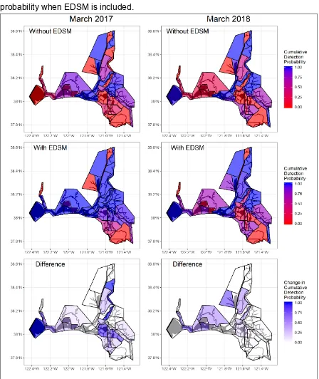
River, and Cache-Slough Liberty Island, with the most dramatic increases occurring in 417
March of each year (Figures 4, A3). 418
419
Discussion
420
Effective management in a dynamic estuarine system can be challenging given 421
the number of species in decline, limited resources, various interacting environmental 422
drivers that continually change the system, and imperfect information to guide 423
management and conservation actions. Monitoring is a crucial component of ecosystem 424
management and leveraging existing data sources for multiple species can be one 425
effective way to enhance information when making management decisions. Here we 426
explored juvenile Chinook Salmon bycatch data collected by the recently established 427
frequency distribution indicates that, in general, fish surveys in the estuary capture similar 429
sizes of juvenile Chinook Salmon from December to March (Figure 2). However, around 430
Chipps Island, Kodiak trawls (as used by EDSM and SKT) appear to be under-sampling 431
larger-sized salmon while DJFMP midwater trawl seems to be under-sampling smaller-432
sized salmon. This is in contrast to a previous study showing that Kodiak trawls catch 433
larger salmon than midwater trawls on the Sacramento River (McLain 1998). The DJFMP 434
midwater trawl used at Chipps Island has a larger net opening and mesh size compared 435
to the DJFMP midwater trawl used on the Sacramento River (Table 1), which may explain 436
this discrepancy (IEP et al. 2019a). If absolute abundance estimation for the various 437
salmon runs in the estuary is the goal (Perry et al. 2016), then a relative gear efficiency 438
assessment using existing data (Walker et al. 2017) or an additional side-by-side gear 439
comparisons for juvenile salmon may be warranted to better understand the fish size bias 440
associated with net and mesh dimensions (Mitchell et al. 2019). 441
The spatiotemporal patterns in occurrence and detectability we observed in our 442
occupancy model were aligned with our understanding of Central Valley salmon life 443
history. We expect to see detection probability increase with salmon density (i.e., number 444
of salmon available to be caught). As such, both occupancy and detection probability 445
estimates were at their highest in February and March−the months in which we would 446
expect higher catch of salmon within our December−March study period (Yoshiyama et 447
al. 1998; Sturrock et al. 2015). Occupancy and detection probability estimates also tend 448
to be higher in regions that are within the migratory pathway of salmon (e.g., Sacramento 449
River, Suisun Bay), whereas backwater areas such as the Sacramento Deep Water 450
Shipping Channel had low cumulative detection probability estimates despite the amount 451
of sampling that occurred (Figure 1). The wet water year of 2017 (December 2016–March 452
2017) saw considerably higher occupancy and detection probabilities (Table A1), 453
consistent with previous studies that demonstrated a positive relationship between 454
outflow and salmon occurrence in the estuary (Kjelson et al. 1982; Brandes and McLain 455
2001; Munsch et al. 2020). In the drier water year of 2018 (December 2017–March 2018), 456
moderate to high occupancy probability estimates were primarily restricted to the 457
survivorship of juvenile salmon along the San Joaquin River and the interior Delta 459
(Newman and Brandes 2010; Perry et al. 2010; Buchanan et al. 2013; Perry et al. 2018). 460
We found considerable differences in detection probability among gear types and 461
these differences remained consistent between the two years. In general, given a single 462
sampling event, beach seines had the highest probability of detecting juvenile Chinook 463
Salmon in a region if the species is present, followed by the fixed station trawl, and then 464
by the EDSM random-station trawl. Multiple factors likely led to this result. Beach seines 465
occur in shallow-water, nearshore habitat, whereas the trawls take place in open water. 466
Juvenile Chinook Salmon may rear in higher density in nearshore habitat than open water 467
(Kjelson et al. 1982). The fixed station trawls that DJFMP conducts (Figure 1) are set in 468
the migratory path of juvenile Chinook Salmon by design, therefore, we can expect these 469
stations to have higher detection probability than randomly chosen sites. It is less clear 470
why fixed sites for a Delta Smelt monitoring program such as the SKT would have higher 471
detection probability for juvenile salmon than those selected at random. However, fixed 472
stations are typically determined based on their higher fish catch and may be comprised 473
of higher quality habitat for fish in general (McClelland and Sass 2012). Random sites as 474
sampled by EDSM are meant to provide a snapshot of the estuary and may inadvertently 475
survey microhabitats not used by juvenile salmon in a particular region. 476
It is also important to consider the assumptions of our model and how they may 477
affect our results. We defined a site as any sub-region with at least a single sample on a 478
given day. Based on our definition, a subregion can become occupied or unoccupied with 479
little consideration for temporal correlation aside from the month variable. This may have 480
biased our occupancy estimates low and our detection probability estimates high, 481
because we may be more likely to classify a subregion as unoccupied if no salmon were 482
caught in a single day, even if salmon were observed in that subregion the day before 483
and after. Moreover, our model assumed that temporal and spatial replicates are 484
comparable. EDSM and DJFMP trawls had temporal replicates, while the SKT and 485
DJFMP beach seines had only spatial replicates (due to the lack of temporal replicates in 486
their original survey designs). This discrepancy may have contributed to some of the 487
differences in the gear detection probabilities we observed. Having spatial replicates may 488
locations within the same subregion and day would likely have more independence (i.e., 490
lower correlation with one another) than multiple samples taken from a single location 491
within the same subregion and day. Teasing apart the different factors that affect 492
detection probability is beyond the scope of our study. However, we expect that the 493
relatively low detection probability of EDSM is partly due to differences in the number of 494
spatial and temporal replicates. 495
Despite the relatively low detection probability of the EDSM trawl, we found 496
substantial improvements in our juvenile Chinook Salmon monitoring coverage for water 497
years 2017 and 2018 (Figures 4, 5). This is largely owed to the wide geographical scope 498
of EDSM and the frequency at which it conducts its sampling. At a single location, EDSM 499
would typically conduct anywhere between two and ten replicate tows, which would 500
increase the program’s cumulative detection probability to levels comparable with other 501
surveys (Figure 3). This was done four days per week throughout December to March in 502
our study period across a large portion of the estuary, resulting in improved cumulative 503
detection probability for juvenile salmon in regions that were generally under-sampled by 504
other surveys (provided that salmon are present in detectable numbers). This added 505
information was most notable in parts of the lower Sacramento River and downstream of 506
the Delta, where EDSM has observed fish that were winter-run and spring-run length-at-507
date sizes. 508
Having information in these key regions of the salmon migratory pathway can help 509
better understand the species’ life history variability (Sturrock et al. 2015; Goertler et al. 510
2018; Sturrock et al. 2020) and how they interact with environmental drivers such as water 511
year type (Figure 5). Moreover, fixed stations are not likely to be representative of the 512
estuary as a whole (IEP SAG 2013; Peterson and Barajas 2018) and may bias abundance 513
estimation (McClelland and Sass 2012; Kiraly et al. 2014; Li et al. 2015). Incorporating 514
random station data from EDSM can potentially aid the estimation of absolute abundance 515
for juvenile Chinook Salmon through the proper calibration of fixed station random effects. 516
Data from EDSM can also be used to better account for imperfect detection (i.e., 517
observation error), as the program’s replicate tows are conducted within a fairly short 518
timeframe and should not violate the closure assumption excessively (Peterson and 519
Chinook Salmon monitoring under the current state. The juvenile Chinook Salmon 521
outmigration window in the estuary extends into the early summer months, and the larval 522
fish gear that EDSM uses in these months does not capture juvenile salmon efficiently. 523
The EDSM program also currently uses length-at-date criteria instead of genetic analysis, 524
which may lead to erroneous assignments for the various Central Valley Chinook Salmon 525
runs (Hedgecock 2002; Harvey et al. 2014). 526
For all fish monitoring programs, there will inevitably be trade‐offs in temporal and 527
spatial scales of measurement due to limited resources and at times, multiple objectives 528
(Radinger et al. 2019). Recommendations have been made to adjust the estuary’s salmon 529
monitoring network, such as the addition of new gears, collection of fish condition 530
information, or transition into randomized stations (IEP SAG 2013; Johnson et al. 2017). 531
Stratified random sampling design offers many advantages and is generally preferable 532
for estimating the abundance of a species given unlimited resources (IEP SAG 2013; 533
Kiraly et al. 2014; Peterson and Barajas 2018). However, results from our model indicate 534
that certain methods (i.e., fixed station beach seines) are more cost-effective at detecting 535
juvenile Chinook Salmon if the species is present in a some areas (as it generally involves 536
less staff and gears). For fixed station surveys, such as the DJFMP beach seine, 537
modifying protocol to include some form of random station selection could provide similar 538
benefits (e.g., high detection probability, cost-effective) while allowing for better 539
abundance estimation. Plans are currently being developed to implement a stratified 540
random sampling design for the DJFMP beach seine survey in accordance with 541
recommendations (IEP SAG 2013), and it would be prudent to assess how detection 542
probabilities change once this new design is implemented. However, for some aspects of 543
juvenile Chinook Salmon management that focus on their occurrence at certain regions, 544
such as the Delta Cross Channel gate operations (NMFS 2009; NMFS 2019), having 545
higher detection probability at specific regions may be more desirable than a proper 546
estimation of abundance. 547
This study serves as a first step in leveraging Delta Smelt monitoring data collected 548
by EDSM to better understand juvenile Chinook Salmon monitoring in the estuary. Our 549
results indicate that using EDSM data along with the traditional salmon surveys can 550
resolution of surveys within each region of the estuary. With data collected under a 552
stratified random design, we can also make better inference on the true proportion of the 553
estuary occupied by salmon at a given time period. Lastly, we demonstrated that trade-554
offs exist between various sampling designs undertaken by the fish monitoring programs 555
we analyzed. By leveraging the strengths from each program, we can make stronger 556
inferences about juvenile Chinook Salmon abundance and distribution patterns. Each 557
survey design (e.g., fixed station vs. random station) offers advantages that are tied to 558
specific monitoring goals. Careful consideration of these trade-offs and the overall 559
monitoring objectives is crucial as management agencies of the estuary continue to adapt 560
and improve their monitoring programs. 561
562
Acknowledgments
563
This work was conducted under the auspices of the Interagency Ecological Program (IEP) 564
for the San Francisco Estuary. Funding was largely provided by the United States Bureau 565
of Reclamation. We thank all past and present staff of the U.S. Fish and Wildlife Service 566
and other IEP agencies who have taken part in the monitoring programs described in our 567
study. We thank staff at the NOAA Fisheries California Central Valley Office, as well as 568
members of the IEP Winter-Run Project Work Team and Science Management Team for 569
their comments and suggestions on early drafts of this study. We also thank Jeffrey 570
McLain, Josh Israel, Page Vick, and Nicole Kwan for valuable feedback on this 571
manuscript. The findings and conclusions of this study are those of the authors and do 572
not necessarily represent the views of our respective agencies. 573
574
References
575 576
Barnett-Johnson R, Grimes CB, Royer CF, Donohoe CJ. 2007. Identifying the 577
contribution of wild and hatchery Chinook Salmon (Oncorhynchus tshawytscha) to the 578
ocean fishery using otolith microstructure as natural tags. Can J Fish Aquat Sci. 579
64:1683–1692. https://doi.org/10.1139/F07-129 580
Brandes PL, McLain JS. 2001. Juvenile Chinook Salmon abundance, distribution, and 581
the Biology of the Central Valley Salmonids. Fish Bulletin. Vol. 2. Sacramento: Calif Dep 583
Fish Game. p. 39–138. 584
Brown LR, May JT. 2006. Variation in spring nearshore resident fish species 585
composition and life histories in the lower San Joaquin watershed and Delta. San Franc 586
Estuary Watershed Sci. [accessed 2014 Nov 4];4(2). 587
https://doi.org/10.15447/sfews.2006v4iss2art1
588
Buchanan RA, Skalski JR, Brandes PL, Fuller A. 2013. Route use and survival of 589
juvenile Chinook Salmon through the San Joaquin River Delta. North Am J Fish Manag. 590
33:216–229. https://doi.org/10.1080/02755947.2012.728178
591
Castillo GC, Damon LJ, Hobbs JA. 2018. Community patterns and environmental 592
associations for pelagic fishes in a highly modified estuary. Mar Coast Fish Dyn Manag 593
Ecosyst Sci. 10:508–524. https://doi.org/10.1002/mcf2.10047 594
Cloern JE, Jassby AD. 2012. Drivers of change in estuarine-coastal ecosystems: 595
Discoveries from four decades of study in the San Francisco Bay. Rev Geophys. 596
50(4):1–33. https://doi.org/10.1029/2012RG000397 597
Cloern JE, Jassby AD, Schraga TS, Nejad E, Martin C. 2017. Ecosystem variability 598
along the estuarine salinity gradient: Examples from long-term study of San Francisco 599
Bay. Limnol Oceanogr. 62:S272–S291. https://doi.org/10.1002/lno.10537 600
Cloern JE, Robinson A, Richey A, Grenier L, Grossinger R, Boyer KE, Burau J, Canuel 601
EA, DeGeorge JF, Drexler JZ, et al. 2016. Primary production in the Delta: Then and 602
now. San Franc Estuary Watershed Sci. [accessed 2016 Oct 21];14(3). 603
https://doi.org/10.15447/sfews.2016v14iss3art1
604
Dege M, Brown LR. 2004. Effect of outflow on spring and summertime distribution and 605
abundance of larval and juvenile fishes in the upper San Francisco Estuary. In: Feyrer 606
F, Brown LR, Brown RL, Orsi JJ, editors. Early life history of fishes in the San Francisco 607
Estuary and watershed. Bethesda: American Fisheries Society. p. 49–65. 608
del Rosario RB, Redler YJ, Newman K, Brandes PL, Sommer T, Reece K, Vincik R. 609
2013. Migration patterns of juvenile winter-run-sized Chinook Salmon (Oncorhynchus 610
Watershed Sci. [accessed 2014 Mar 26];11(1). 612
https://doi.org/10.15447/sfews.2013v11iss1art3 613
Fisher FW. 1992. Chinook Salmon, Oncorhynchus tshawytscha, growth and occurrence 614
in the Sacramento-San Joaquin River system. Redding (CA): Calif Dep Fish Wildl, 615
Inland Fisheries Division. 616
Fiske IJ, Chandler RB. 2011. Unmarked: An R package for fitting hierarchical models of 617
wildlife occurrence and abundance. J Stat Softw. 43(10):1–23. 618
https://doi.org/10.18637/jss.v043.i10
619
Goertler PAL, Sommer TR, Satterthwaite WH, Schreier BM. 2018. Seasonal floodplain- 620
tidal slough complex supports size variation for juvenile Chinook Salmon 621
(Oncorhynchus tshawytscha). Ecol Freshw Fish. 27(2):580–593. 622
https://doi.org/10.1111/eff.12372
623
Harvey BN, Jacobson DP, Banks MA. 2014. Quantifying the uncertainty of a juvenile 624
Chinook Salmon race identification method for a mixed-race stock. North Am J Fish 625
Manag. 34(6):1177–1186. https://doi.org/10.1080/02755947.2014.951804
626
Hedgecock D. 2002. Microsatellite DNA for the management and protection of 627
California’s Central Valley Chinook Salmon (Oncorhynchus tshawytscha). Final Report 628
for the Amendment to Agreement No. B‐59638. Report prepared for California 629
Department of Water Resources. Davis (CA): University of California, Bodega Marine 630
Laboratory. 631
Huber ER, Carlson SM. 2015. Temporal trends in hatchery releases of fall-run Chinook 632
Salmon in California’s Central Valley. San Franc Estuary Watershed Sci. [accessed 633
2016 May 10];13(2). https://doi.org/10.15447/sfews.2015v13iss2art3
634
[IEP SAG] Interagency Ecological Program Science Advisory Group. 2013. Review of 635
the IEP Delta Juvenile Fishes Monitoring Program and Delta Juvenile Salmonid Survival 636
Studies. Sacramento (CA): Interag Ecol Progr. 637
[IEP et al.] Interagency Ecological Program, Mahardja B, Speegle J, Nanninga A, 638
Barnard D. 2019a. Interagency Ecological Program: Over four decades of juvenile fish 639
Monitoring Program, 1976–2018 ver 3. Environmental Data Initiative; [accessed 2019 641
Aug 10]. https://doi.org/10.6073/pasta/87dda12bed2271ce3d91abdb7864c50c
642
[IEP et al.] Interagency Ecological Program, Schreier B, Davis B, Ikemiyagi N. 2019b. 643
Interagency Ecological Program: Fish catch and water quality data from the Sacramento 644
River floodplain and tidal slough, collected by the Yolo Bypass Fish Monitoring 645
Program, 1998–2018. Environmental Data Initiative; [accessed 2018 Dec 27]. 646
https://doi.org/10.6073/pasta/b0b15aef7f3b52d2c5adc10004c05a6f
647
Johnson RC, Windell S, Brandes PL, Conrad JL, Ferguson J, Goertler PAL, Harvey BN, 648
Heublein J, Israel JA, Kratville DW, et al. 2017. Science advancements key to 649
increasing management value of life stage monitoring networks for endangered 650
Sacramento River winter-run Chinook Salmon in California. San Franc Estuary 651
Watershed Sci. [accessed 2017 Oct 4];15(3). 652
https://doi.org/10.15447/sfews.2017v15iss3art1
653
Joseph LN, Maloney RF, Possingham HP. 2009. Optimal allocation of resources among 654
threatened species: a project prioritization protocol. Conserv Biol. 23(2):328–338. 655
https://doi.org/10.1111/j.1523-1739.2008.01124.x
656
Julienne J. 2016. Timing, composition, and abundance of juvenile salmonid emigration 657
in the Sacramento River near Knights Landing October 2012−Devember 2012. 658
Sacramento (CA): Calif Dep Fish Wildl. 659
Kampstra P. 2008. Beanplot: A boxplot alternative for visual comparison of distributions. 660
J Stat Softw. 28. https://doi.org/10.18637/jss.v028.c01
661
Kennish MJ. 2002. Environmental threats and environmental future of estuaries. 662
Environ Conserv. 29:78–107. https://doi.org/10.1017/S0376892902000061
663
Kimmerer WJ, Gross ES, MacWilliams ML. 2009. Is the response of estuarine nekton to 664
freshwater flow in the San Francisco Estuary explained by variation in habitat volume? 665
Estuar Coast. 32:375–389. https://doi.org/10.1007/s12237-008-9124-x
666
Kiraly IA, Coghlan Jr. SM, Zydlewski J, Hayes D. 2014. Comparison of two sampling 667
designs for fish assemblage assessment in a large river. Trans Am Fish Soc. 143:508– 668
518. https://doi.org/10.1080/00028487.2013.864706
Kjelson MA, Raquel PF, Fisher FW. 1982. Life history of fall-run juvenile Chinook 670
Salmon, Oncorhynchus tshawytscha, in the Sacramento-San Joaquin Estuary, 671
California. In: Kennedy VS, editor. Estuarine Comparisons. New York (NY): Academic 672
Press. p. 393–411. 673
Li B, Cao J, Chang J-H, Wilson C, Chen Y. 2015. Evaluation of effectiveness of fixed-674
station sampling for monitoring American Lobster settlement. North Am J Fish Manag. 675
35:942–957. https://doi.org/10.1080/02755947.2015.1074961
676
Lund J, Hanak E, Fleenor W, Bennett W, Howitt R, Mount J, Moyle P. 2008. Comparing 677
futures for the Sacramento-San Joaquin Delta. San Francisco: Public Policy Institute of 678
California. 679
Lund JR. 2016. California’s agricultural and urban water supply reliability and the 680
Sacramento-San Joaquin Delta. San Franc Estuary Watershed Sci. [accessed 2019 681
Sep 21];14(3). https://doi.org/10.15447/sfews.2016v14iss3art6
682
MacKenzie DI, Nichols JD, Lachman GB, Droege S, Royle JA, Langtimm CA. 2002. 683
Estimating site occupancy rates when detection probabilities are less than one. 684
Ecology. 83(8):2248–2255.
https://doi.org/10.1890/0012-685
9658(2002)083[2248:ESORWD]2.0.CO;2 686
Mahardja B, Farruggia MJ, Schreier B, Sommer T. 2017. Evidence of a shift in the 687
littoral fish community of the Sacramento-San Joaquin Delta. PLoS One. [accessed 688
2017 Jan 24];12(1). https://doi.org/10.1371/journal.pone.0170683 689
McClelland MA, Sass GG. 2012. Assessing fish collections from random and fixed site 690
sampling methods on the Illinois River. J Freshw Ecol. 27(3):325–333. 691
https://doi.org/10.1080/02705060.2012.658213 692
McLain J. 1998. Relative efficiency of the midwater and Kodiak trawl at capturing 693
juvenile Chinook Salmon in the Sacramento River. Interag Ecol Progr Newsl. 11(4):26– 694
29. 695
Mitchell L, Newman K, Baxter R. 2017. A covered cod-end and tow-path evaluation of 696
midwater trawl gear efficiency for catching Delta Smelt (Hypomesus transpacificus). 697
https://doi.org/10.15447/sfews.2017v15iss4art3 699
Mitchell L, Newman K, Baxter R. 2019. Estimating the size selectivity of fishing trawls 700
for a short-lived fish species. San Franc Estuary Watershed Sci. [accessed 2019 Mar 701
15];17(1). https://doi.org/10.15447/sfews.2019v17iss1art5 702
Moyle PB. 2002. Inland fishes of California. Berkeley (CA): University of California 703
Press. 704
Moyle PB, Hobbs JA, Durand JR. 2018. Delta Smelt and water politics in California. 705
Fisheries. 43(1):42–50. https://doi.org/10.1002/fsh.10014 706
Munsch SH, Greene CM, Johnson RC, Satterthwaite WH, Imaki H, Brandes PL, 707
O’Farrell MR. 2020. Science for integrative management of a diadromous fish stock: 708
interdependencies of fisheries, flow, and habitat restoration. Can J Fish Aquat Sci. 709
Accepted. 710
Newman KB, Brandes PL. 2010. Hierarchical modeling of juvenile Chinook Salmon 711
survival as a function of Sacramento-San Joaquin Delta water exports. North Am J Fish 712
Manag. 30:157–169. https://doi.org/10.1577/M07-188.1 713
Nichols FH, Cloern JE, Luoma SN, Peterson DH. 1986. The modification of an estuary. 714
Science. 231:567–573. https://doi.org/10.1126/science.231.4738.567 715
[NMFS] National Marine Fisheries Service. 2009. Biological opinion and conference 716
opinion on the long-term operations of the Central Valley and State Water Project. 717
National Marine Fisheries Service, Southwest Region. 718
[NMFS] National Marine Fisheries Service. 2019. Biological Opinion on Long-term 719
Operation of the Central Valley Project and the State Water Project. National Marine 720
Fisheries Service, Southwest Region. Available from: 721
https://repository.library.noaa.gov/view/noaa/22046 722
Perry RW, Buchanan RA, Brandes PL, Burau JR, Israel JA. 2016. Anadromous 723
salmonids in the Delta: new science 2006–2016. San Franc Estuary Watershed Sci. 724
[accessed 2018 Apr 25];14(2). https://doi.org/10.15447/sfews.2016v14iss2art7 725
Chinook Salmon in a spatially complex, tidally forced river delta. Can J Fish Aquat Sci. 728
75(11):1886–1901. https://doi.org/10.1139/cjfas-2017-0310 729
Perry RW, Skalski JR, Brandes PL, Sandstrom PT, Klimley AP, Ammann A, 730
MacFarlane B. 2010. Estimating survival and migration route probabilities of juvenile 731
Chinook Salmon in the Sacramento-San Joaquin River Delta. North Am J Fish Manag. 732
30:142–156. https://doi.org/10.1577/M08-200.1 733
Peterson JT, Barajas MF. 2018. An evaluation of three fish surveys in the San 734
Francisco Estuary, California, 1995–2015. San Franc Estuary Watershed Sci. 735
[accessed 2018 Dec 27];4(2). https://doi.org/10.15447/sfews.2018v16iss4art2 736
Polansky L, Newman KB, Nobriga ML, Mitchell L. 2018. Spatiotemporal models of an 737
estuarine fish species to identify patterns and factors impacting their distribution and 738
abundance. Estuar Coast. 41:572–581. https://doi.org/10.1007/s12237-017-0277-3 739
R Core Team. 2018. A language and environment for statistical computing. 740
https://www.r-project.org/ 741
Radinger J, Britton JR, Carlson SM, Magurran AE, Alcaraz-Hernandez JD, Almodovar 742
A, Benejam L, Fernandez-Delgado C, Nicola GG, Oliva-Paterna FJ, et al. 2019. 743
Effective monitoring of freshwater fish. Fish and Fisheries. 20(4):729–747. 744
https://doi.org/10.1111/faf.12373 745
Reynolds FL, Mills TJ, Benthin R, Low A. 1993. Restoring Central Valley Streams: A 746
Plan for Action. Sacramento (CA): Calif Dep Fish Game. 747
Snider B, Titus RG. 2000. Timing, composition, and abundance of juvenile anadromous 748
salmonid emigration in the Sacramento River near Knights Landing October 749
1998−September 1999. Sacramento (CA): Calif Dep Fish Game. 750
Souza, K. 2002. Revision of California Department of Fish and Game's Spring Midwater 751
Trawl and results of the 2002 Spring Kodiak Trawl.Interag Ecol Progr Newsl. 15(3):44– 752
47. 753
Stevens DE, Miller LW. 1983. Effects of river flow on abundance of young Chinook 754
Salmon, American Shad, Longfin Smelt, and Delta Smelt in the Sacramento-San 755
Stevens DL, Olsen AR. 2004. Spatially balanced sampling of natural resources. J Am 757
Stat Assoc. 99(465):262–278. https://doi.org/10.1198/016214504000000250 758
Sturrock AM, Carlson SM, Wikert JD, Heyne T, Nussle S, Merz JE, Sturrock HJW, 759
Johnson RC. 2020. Unnatural selection of salmon life histories in a modified riverscape. 760
Glob Chang Biol. 26:1235–1247. https://doi.org/10.1111/gcb.14896 761
Sturrock AM, Satterthwaite WH, Cervantes-Yoshida KM, Huber ER, Sturrock HJW, 762
Nussle S, Carlson SM. 2019. Eight decades of hatchery salmon releases in the 763
California Central Valley: Factors influencing straying and resilience. Fisheries. 764
44(9):433–444. https://doi.org/10.1002/fsh.10267 765
Sturrock AM, Wikert JD, Heyne T, Mesick C, Hubbard AE, Hinkelman TM, Weber PK, 766
Whitman GE, Glessner JJ, Johnson RC. 2015. Reconstructing the migratory behavior 767
and long-term survivorship of juvenile Chinook Salmon under contrasting hydrologic 768
regimes. PLoS One. [accessed 2018 Apr 25];10(5). 769
https://doi.org/10.1371/journal.pone.0122380 770
Thomson JR, Kimmerer WJ, Brown LR, Newman KB, Mac Nally R, Bennett WA, Feyrer 771
F, Fleishman E. 2010. Bayesian change point analysis of abundance trends for pelagic 772
fishes in the upper San Francisco Estuary. Ecol Appl. 20(5):1431–1448. 773
https://doi.org/10.1890/09-0998.1 774
[USFWS] United States Fish and Wildlife Service, Johnston C, Lee S, Mahardja B, 775
Speegle J, Barnard D. 2019. U.S. Fish and Wildlife Service: San Francisco Estuary 776
Enhanced Delta Smelt Monitoring Program data, 2016–2019. Environmental Data 777
Initiative; [accessed 2019 Aug 27]. 778
https://doi.org/10.6073/pasta/98bce400502fae3a6b77b3e96f6d51e7 779
Walker ND, Maxwell DL, Le Quesne WJF, Jennings S. 2017. Estimating efficiency of 780
survey and commercial trawl gears from comparisons of catch-ratios. ICES J Mar Sci. 781
74(5):1448–1457. https://doi.org/10.1093/icesjms/fsw250 782
Whipple A, Grossinger R, Rankin D, Stanford B, Askevold R. 2012. Sacramento-San 783
Joaquin Delta historical ecology investigation: Exploring pattern and process. San 784
Estuary Institute. Available at:
https://www.sfei.org/documents/sacramento-san-joaquin-786
delta-historical-ecology-investigation-exploring-pattern-and-proces 787
Willmes M, Hobbs JA, Sturrock AM, Bess Z, Lewis LS, Glessner JJG, Johnson RC, 788
Kurth R, Kindopp J. 2018. Fishery collapse, recovery, and the cryptic decline of wild 789
salmon on a major California river. Can J Fish Aquat Sci. 75:1836–1848. 790
https://doi.org/10.1139/cjfas-2017-0273 791
Yoshiyama RM, Fisher FW, Moyle PB. 1998. Historical Abundance and Decline of 792
Chinook Salmon in the Central Valley Region of California. North Am J Fish Manag. 793
18:487–521. https://doi.org/10.1577/1548-8675(1998)018<0487:HAADOC>2.0.CO;2. 794
Figures and Tables
797Figure 1. Map of the study area including random sites sampled by EDSM during the study period (December 2016 – March 798
2017 and December 2017–March 2018), fixed stations sampled by other monitoring programs used in this study, the 11 799
regions used for occupancy modeling (in dark blue lines), and the 39 subregions (in grey lines) used to calculate across-800
gear cumulative detection probability. 801
Figure 2. Series of bean plots comparing the size distribution of juvenile Chinook Salmon 804
caught in EDSM Kodiak trawl relative to the SKT survey and three DJFMP methods. The 805
bandwidth for all bean plots was set to 5 and the median fork length highlighted by the 806
solid horizontal black line. Catch counts are illustrated by stacked histograms within each 807
density distribution polygon. 808
Figure 3. Results from occupancy model demonstrating juvenile Chinook Salmon 812
cumulative detection probability by EDSM Kodiak trawl relative to other gears from the 813
Upper Sacramento River subregion in water year of 2018. Attempt number denotes the 814
number of “replicates”. 815
828
Figure 4. Cumulative detection probability summary (assuming salmon presence) by 829
subregion for March of 2017 and 2018 demonstrating increased spatial coverage for 830
juvenile Chinook Salmon through EDSM for both high (2017) and low (2018) density 831
years. The top and middle rows show cumulative detection probabilities without and with 832
the inclusion of EDSM sampling while the bottom row shows the resulting difference in 833
Figure 5. Size and life stages of Chinook Salmon caught in EDSM Kodiak trawls from Suisun Bay, Suisun Marsh, and San 836
Pablo Bay regions (as seen in Figure 1), demonstrating contrast in numbers and sizes of Chinook Salmon observed within 837
this area between the wet water year of 2017 and moderately dry year of 2018. Only data from measured fish are shown 838
on the figure. Colors denote different life stages of Chinook Salmon as classified by field crew and “n/p” indicates that it was 839
not recorded (generally for adipose fin-clipped, hatchery fish). 840
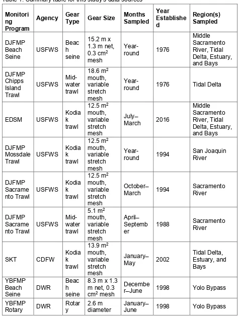
Table 1. Summary table for this study’s data sources 842 Monitori ng Program
Agency Gear Type Gear Size Months Sampled Year Establishe d
Region(s) Sampled
DJFMP Beach
Seine USFWS
Beac h seine
15.2 m x 1.3 m net, 0.3 cm2 mesh
Year-round 1976
Middle Sacramento River, Tidal Delta, Estuary, and Bays DJFMP Chipps Island Trawl
USFWS Mid-water trawl
18.6 m2 mouth, variable stretch mesh
Year-round 1976 Tidal Delta
EDSM USFWS Kodiak trawl
12.5 m2 mouth, variable stretch mesh
July ̶
March 2016
Middle Sacramento River, Tidal Delta, Estuary, and Bays DJFMP Mossdale
Trawl USFWS
Kodia k trawl
12.5 m2 mouth, variable stretch mesh
Year-round 1994 San Joaquin River
DJFMP Sacrame
nto Trawl USFWS
Kodia k trawl
12.5 m2 mouth, variable stretch mesh
October ̶
March 1994 Sacramento River
DJFMP Sacrame
nto Trawl USFWS
Mid-water trawl
5.1 m2 mouth, variable stretch mesh
April ̶ Septemb
er 1988
Sacramento River
SKT CDFW Kodiak trawl
13.9 m2 mouth, variable stretch mesh
January ̶
May 2002
Tidal Delta, Estuary, and Bays
YBFMP Beach
Seine DWR
Beac h seine
8.3 m x 1.3 m net, 0.3 cm2 mesh
Decembe
r ̶ June 1998 Yolo Bypass YBFMP
Screw
Trap screw trap rotary screw trap Knights
Landing Rotary Screw Trap
CDFW
Rotar y screw trap
2.4 m diameter rotary screw trap
October–
June 1995 Sacramento River
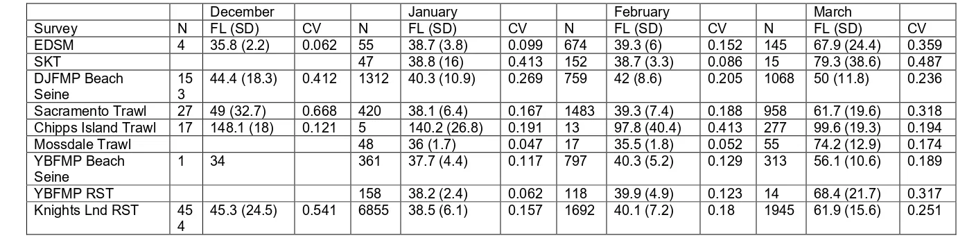
Table 2: Total number of Chinook Salmon captured (N), average fork length in mm (FL) and standard deviation (SD), and 844
coefficient of variation of fish fork length (CV) by each survey during our study period (December 2016 – March 2017, 845
December 2017 – March 2018). Surveys included EDSM, DJFMP, Spring Kodiak Trawl (SKT), Yolo Bypass Fish Monitoring 846
Program (YBFMP), and the Knights Landing (Knights Lnd) Rotary Screw Traps (RST). Note: Data exclude adipose-clipped 847
Chinook Salmon. 848
849
December January February March
Survey N FL (SD) CV N FL (SD) CV N FL (SD) CV N FL (SD) CV
EDSM 4 35.8 (2.2) 0.062 55 38.7 (3.8) 0.099 674 39.3 (6) 0.152 145 67.9 (24.4) 0.359
SKT 47 38.8 (16) 0.413 152 38.7 (3.3) 0.086 15 79.3 (38.6) 0.487
DJFMP Beach
Seine 153 44.4 (18.3) 0.412 1312 40.3 (10.9) 0.269 759 42 (8.6) 0.205 1068 50 (11.8) 0.236
Sacramento Trawl 27 49 (32.7) 0.668 420 38.1 (6.4) 0.167 1483 39.3 (7.4) 0.188 958 61.7 (19.6) 0.318
Chipps Island Trawl 17 148.1 (18) 0.121 5 140.2 (26.8) 0.191 13 97.8 (40.4) 0.413 277 99.6 (19.3) 0.194
Mossdale Trawl 48 36 (1.7) 0.047 17 35.5 (1.8) 0.052 55 74.2 (12.9) 0.174
YBFMP Beach
Seine 1 34 361 37.7 (4.4) 0.117 797 40.3 (5.2) 0.129 313 56.1 (10.6) 0.189
YBFMP RST 158 38.2 (2.4) 0.062 118 39.9 (4.9) 0.123 14 68.4 (21.7) 0.317
Knights Lnd RST 45
4 45.3 (24.5) 0.541 6855 38.5 (6.1) 0.157 1692 40.1 (7.2) 0.18 1945 61.9 (15.6) 0.251