1 Understanding UCEs: A comprehensive primer on using Ultraconserved Elements for 1
arthropod phylogenomics 2
3
Y. Miles Zhang*, Jason L. Williams, Andrea Lucky 4
University of Florida, Department of Entomology & Nematology, Gainesville, FL, 32608 5
* Corresponding author email: [email protected] 6
Abstract:
7
Targeted enrichment of ultraconserved elements (UCE) has emerged as a promising tool for
8
inferring evolutionary history in many taxa, with utility ranging from phylogenetic and
9
phylogeographic questions at deep time scales to population level studies at shallow time scales.
10
However, the methodology can be daunting for beginners. Our goal is to introduce UCE
11
phylogenomics to a wider audience by summarizing recent advances in arthropod research, and
12
to familiarize readers with background theory and steps involved. We define terminology used in
13
association with the UCE approach, evaluate current laboratory and bioinformatic methods and
14
limitations, and, finally, provide a roadmap of steps in the UCE pipeline to assist
15
phylogeneticists in making informed decisions as they employ this powerful tool. By facilitating
16
increased adoption of UCE in phylogenomics studies that deepen our comprehension of the
17
function of these markers across widely divergent taxa, we aim to ultimately improve
18
understanding of the arthropod tree of life.
19
Keywords: Arachnida, Insecta, Phylogenomics Methods, Target Enrichment, 20
Ultraconserved Elements 21
2 22
Introduction & Background
23
The advent of massively-parallel sequencing technology and the subsequent emergence
24
of the field of phylogenomics has invigorated evolutionary biology in a relatively short time span
25
(reviewed in Philippe et al. 2011, Jones and Good 2016). This molecular revolution has offered
26
unprecedented opportunities to generate large-scale datasets, and with the concurrent explosion
27
of analytic and bioinformatics tools, has made it possible to address previously intractable
28
challenges due to limited genetic markers. However, the rapidity with which new technologies
29
have emerged has made it difficult for scientists to stay up to date about useful new tools;
30
understanding the steps involved in using new methods presents a challenge for researchers.
31
Genome-scale studies are rapidly supplanting the Sanger sequencing-based, multi-locus
32
molecular phylogenetic methods that dominated from the mid-1990’s through the early 2000’s;
33
today, genomic-scale studies dwarf previous approaches in the sheer scale of data they generate
34
(Bravo et al. 2019). While the cost and scale of whole-genome sequencing are prohibitive for
35
many researchers, recent advances in sequencing technology and laboratory protocols have made
36
it possible to generate high quality genomic datasets using a combination of next-generation
37
sequencing, genomic reduction, and sample multiplexing (Lemmon and Lemmon 2013,
38
McCormack et al. 2013a). These so-called ‘genome reduction’ or ‘reduced representation’
39
approaches can rapidly generate datasets with thousands of loci, at relatively low cost, for model
40
and non-model taxa alike. Methods such as restriction enzyme-associated DNA sequencing
41
(RADseq; Miller et al. 2007, Baird et al. 2008, Peterson et al. 2012), transcriptomics (Bi et al.
42
2012), and target enrichment methods such as Anchored Hybrid Enrichment (AHE) (Lemmon et
3
al. 2012) or target capture of Ultraconserved Elements (UCE) (Faircloth 2017) are now widely
44
used for generating genomic-scale data for phylogenomic studies. These phylogenomics methods
45
are similar in some respects, but each has strengths and weaknesses which may not be easily
46
discerned by researchers new to this field. Because of the proliferation of new approaches and
47
tools in phylogenetics, selecting a method to use in the era of ‘big data’ can be daunting.
48
Potential users need guidance in choosing methods appropriate to their research questions, and in
49
navigating confusing terminologies, bioinformatics-heavy data processing, and computationally
50
intensive analyses.
51
UCE-based phylogenomics continues to develop rapidly, and the lack of comprehensive
52
review has been a significant challenge for potential users to overcome when exploring this
53
option. This paper summarizes recent advances in UCE phylogenomics in arthropod research;
54
we start by familiarizing readers with background theory and terminology, and describing the
55
steps involved in generating and analyzing UCE data, and then provide quality-control tips to
56
ensure that data collection and downstream analyses can be performed with confidence.
57
58
What are UCEs? 59
Ultraconserved Elements are highly-conserved regions within the genome that are shared
60
among evolutionarily distant taxa (Bejerano et al. 2004). The DNA adjacent to each ‘core’ UCE
61
region, known as flanking DNA, increases in variability with distance from the region (Faircloth
62
et al. 2012). UCEs and flanking regions can be selectively captured, and used to reconstruct the
63
evolutionary history of taxa at various time scales, from deep to shallow phylogenetic
64
divergences (Faircloth et al. 2012, McCormack et al. 2012).
4
The UCE approach belongs to the broad category of ‘target enrichment’ phylogenomic
66
techniques, which involve selective capture of genomic regions from DNA prior to sequencing
67
(Mamanova et al. 2010). Similar methods include AHE (Anchored Hybrid Enrichment),
68
BaitFisher (Mayer et al. 2016), and Hyb-Seq (Weitemier et al. 2014). AHE has been the most
69
widely used method for animal studies, to date, but all target enrichment methods have been
70
successfully used across a variety of taxa. These techniques universally involve identifying loci
71
of interest, then designing custom-made molecular probes (also known as baits) which are
72
hybridized to loci of interest, and ultimately sequencing selected genomic region on a
massively-73
parallel platform. The main difference between the AHE and UCE approaches is the nature of
74
the loci targeted; AHE focuses on fewer loci (300-600) that are exclusively exonic, while UCEs
75
target more loci (>1000) using fewer probes – these may include both exonic and intronic
76
regions, depending on the organism (Crawford et al. 2012, McCormack et al. 2012, Faircloth et
77
al. 2015). While AHE can cope with sequence variation at target loci by using a more diverse set
78
of probes per locus, the details of the methodology are not available for scrutiny as they are, in
79
part, proprietary (Lemmon et al. 2012). The UCE approach, in contrast, is fully open source,
80
which has contributed to recent interest in using these markers for arthropod phylogenomics.
81
82
Advantages of UCE Phylogenomics 83
The UCE approach has become an increasingly popular target enrichment method for
84
generating phylogenomic data, as it offers advantages over traditional Sanger sequencing
85
methods in terms of quantity of data generated. UCEs have successfully been used in studies
86
across a broad array of animal taxa including birds (McCormack et al. 2013b, Musher and
87
Cracraft 2018), mammals (McCormack et al. 2012, Mclean et al. 2018), fish (Faircloth et al.
5
2013, Alda et al. 2018), amphibians (Newman and Austin 2016, Zarza et al. 2018), reptiles
89
(Crawford et al. 2012, Streicher and Wiens 2017, Myers et al. 2019), sponges (Ryu et al. 2012),
90
cnidarians (Quattrini et al. 2018), echindoderms (Ryu et al. 2012), and arthropods (Faircloth et
91
al. 2015, Baca et al. 2017b, Branstetter et al. 2017c, Hedin et al. 2018b, Kieran et al. 2019).
92
These studies range widely in evolutionary scale, from phylogenetic and phylogeographic
93
questions at deep time scales (Faircloth et al. 2013, Smith et al. 2014, Branstetter et al. 2017c) to
94
population level studies at shallow time scales (Harvey et al. 2016, Manthey et al. 2016, Zarza et
95
al. 2018, Branstetter and Longino 2019, Myers et al. 2019).
96
Benefits of using UCE include openly shared resources such as probe sets
97
(https://www.ultraconserved.org/), lab protocols (https://baddna.uga.edu/protocols.html/), and
98
bioinformatics tools (https://phyluce.readthedocs.io/en/latest/), making it an easy method to learn
99
and use in comparison to more proprietary alternatives such as AHE. Complete library
100
preparation for around 100 samples can be completed in approximately two weeks by one
101
person, or a month if counting DNA extraction and possible troubleshooting. UCE datasets can
102
be easily standardized, even from multiple studies, by using the same probe set. In this way, data
103
from studies using the same probe set or with exon/transcriptome data (Bossert et al. 2019,
104
Kieran et al. 2019) can be combined and can incorporate legacy methods if the probe set includes
105
Sanger genes (Branstetter et al. 2017a). These are distinct advantages over restriction
enzyme-106
based methods such as traditional RADseq, which lacks repeatability due to the random nature of
107
the restriction enzyme digestion that generates random genomic fragments. An additional
108
advantage of target enrichment methods is the high success rate with degraded or low-quantity
109
samples; older, dried museum specimens may be unusable in traditional restriction
enzyme-110
based and transcriptomics studies as they require large quantities of high-quality DNA or RNA
6
from fresh or carefully-preserved tissues (Blaimer et al. 2016a, Lim and Braun 2016, Ruane and
112
Austin 2017). It is worth noting that newer RAD-based methods such as RADcap (Hoffberg et
113
al. 2016), Rapture (Ali et al. 2016), and hyRAD (Suchan et al. 2016) address these limitations by
114
using a combination of restriction enzyme digestion and hybridization capture probes to
115
overcome traditional RAD-based problems such as allele dropout, and can successfully capture
116
degraded DNA from older museum samples.
117
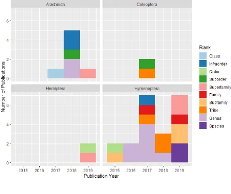
UCE and Arthropods 118
The UCE approach was first demonstrated outside of vertebrates in the insect order
119
Hymenoptera (See Table 1). To date, two published probe sets exist for Hymenoptera: hym-v2
120
(31,829 probes for 2,590 UCEs, Branstetter et al. 2017a) includes most of the original hym-v1
121
probe sets (2,749 probes for 1,510 UCEs, Faircloth et al. 2015), and excludes poorly performing
122
loci. Other arthropods groups for which published UCE data exist include Arachnida,
123
Coleoptera, and Hemiptera; as well as multiple upcoming studies for Diptera (E. Buenaventura,
124
C. Cohen, K. Noble, pers. comm.). Psocodea and Lepidoptera probe sets have been developed
125
but not yet tested in vitro (Table 1). The utility of UCEs extends beyond purely phylogenetic and
126
taxonomic research. For example, UCE-based community phylogenomics has been used to
127
reveal the importance of bee phylodiversity in agriculture (Grab et al. 2019); UCE-based
128
phylogeny and geometric morphometrics have been used in combination to explore the evolution
129
of parasitic wasp body shape (Santos et al. 2019); single nucleotide polymorphisms (SNPs)
130
generated from UCE data have been used to demonstrate the success of unsupervised machine
131
learning in species delimitation of harvestmen (Derkarabetian et al. 2019), and UCE phylogenies
132
have been integrated with environmental niche modeling to examine phylogeographic patterns of
133
ants across the Brazilian Atlantic Forest (Ströher et al. 2019).
7
This study compiles all currently available UCE-based literature related to arthropods as
135
of July 2019 (n = 32, Figure 1), but will undoubtedly increase exponentially in the future (Table
136
1). Our aim is to provide a step-by-step guide to make the UCE research pipeline more
137
approachable to researchers working across different arthropod groups.
138
139
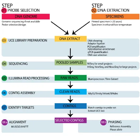
UCE Phylogenomics Pipeline
140
The steps in the UCE pipeline are 1) probe selection and design; 2) wet lab work and
141
sequencing; 3) bioinformatics; and 4) phylogenomic analyses. Below, we visualize the process in
142
a workflow diagram (Figure 2) and describe the choices a researcher must make at each stage. A
143
glossary of technical terms is provided as a supplementary document (S1).
144
145
Probe Selection & Design 146
Probe sets are a collection of oligonucleotides that will bind to specific, conserved
147
genome regions of interest, often called baits as they can ‘fish’ out the region of interest. These
148
probes are sometimes interchangeably called ‘baits’ as they are used to fish out target loci from a
149
‘pond’ of randomly sheared, adaptor-ligated DNA (Gnirke et al. 2009). However, to avoid
150
confusion we recommend reserving the term ‘baits’ for the intermediate stage in probe design;
151
by contrast, ‘probes’ refer to the final products that is synthesized for commercial use (Gustafson
152
et al. 2019). A probe set functions through a collection of biotinylated oligonucleotides that are
153
designed to bind with specific genome regions of interest. Probes are combined with denatured
154
and cooled DNA, allowing for ‘in solution’ hybridization to targets. Streptavidin-coated
8
magnetic beads, which have high affinity for biotin, are added into the solution. The beads then
156
bind to the probe-DNA hybrids through the biotin on the probe set. Any unwanted DNA
157
fragments are then washed away, leaving only the desired regions attached to the beads (Gnirke
158
et al. 2009).
159
Probes are designed based on UCE loci identified from published genomes for each
160
taxonomic group. Currently probe sets for Arachnida, Coleoptera, Diptera, Hemiptera, and
161
Hymenoptera are available for purchase through Arbor Biosciences
162
(https://arborbiosci.com/products/uces/). Other taxonomic groups either have no probe sets
163
available, or have not been tested in vitro. Designing new probe sets may prove challenging in
164
the absence of published genomes for a group of interest. Nevertheless, low coverage genome
165
sequencing (5x) may be an increasingly affordable appropriate first step (Zhang et al. 2019). The
166
sequenced genomes selected as the basis for probe design should ideally reflect diversity within
167
the group of interest. Ideally multiple genomes should be used for probe design, but minimally
168
probe sets designed based on only two genomes (hym-v1) were shown to be successful in
169
capturing UCEs across the diverse order Hymenoptera (Faircloth et al. 2015).
170
Whereas probe selection is straightforward (they are either available for the group of
171
interest or they are not), probe design for new taxonomic groups is a time-consuming process for
172
any target enrichment method, as the probe sets can differ in number and composition depending
173
on the target taxa and evolutionary scale. Currently published probe sets for arthropods target
174
1,100 – 2,700 UCEs loci, and have been made publicly available under public domain license
175
(CC-0), thus allowing for restriction-free commercial synthesis, testing, use and improvements
176
by other research groups (http://ultraconserved.org/#protocols) (Branstetter et al. 2017a,
177
Faircloth 2017, Gustafson et al. 2019). A generalized workflow for identifying conserved
9
sequences shared among divergent genomes and enrichment probes design is available (Faircloth
179
2017), and a new pipeline has been described using low-coverage genome sequencing that can
180
also be used to design UCE probes (Zhang et al. 2019). In brief, the probe design sequence is 1)
181
select base genome (s); 2) generate short reads as exemplars of the focal group’s diversity and
182
align to base genome(s); 3) merge approximate reads and find overlapping regions shared among
183
exemplar taxa and base genome (conserved regions); 4) design temporary bait set from base
184
genome against conserved regions and align to exemplar genome assemblies to remove
185
duplicates; 5) design exemplar-specific probes for each locus where temporary baits match
186
exemplar genome assemblies.
187
How to best optimize the probe design process is an area of active research. Both base
188
genome choice and initial bait design stringency parameters can greatly affect the number of
189
resultant probes and, subsequently, the number of loci detected and recovered in Adephagan
190
beetles (Gustafson et al. 2019). The optimal base genome can be selected by conducting a base
191
genome experiment by iteratively selecting each taxon as the base genome and finding candidate
192
loci shared among exemplar taxa, or selected from taxon with the smallest average genetic
193
distance to the other exemplar taxa through independently generated Sanger markers. Probe sets
194
can also be modified to incorporate additional loci. The Hymenoptera probe set hym-v1 was
195
improved by the publication of hym-v2, which included most of the original hym-v1 loci as well
196
as new loci and probes targeting 16 commonly-sequenced nuclear genes to allow for ‘back
197
compatibility’ with Sanger-era data (Branstetter et al. 2017a). The resulting capability of
198
combining new genomic data with older sequences obtained from ‘legacy’ markers is vital to
199
phylogenetic studies, as DNA quality tissue for many rare but vital taxa to phylogenetic studies
200
may be difficult or impossible to obtain repeatedly. In silico tests of existing probe sets
10
demonstrate moderate success with sister outgroups, such as using the Hemiptera probe set to
202
capture UCEs from thrips (Insecta, Order: Thysanoptera) (Faircloth 2017). Importantly, expense,
203
time, and computational resources needed should be taken into consideration when designing
204
new probe sets. The cost of development should be weighed against the potential future use of
205
the probe set beyond the initial study; UCE probes for larger clades, for example, may be more
206
likely to be adopted for multiple uses than those designed for species-poor groups.
207
Wet Lab Work & Sequencing 208
Specimen selection and DNA extraction. Selecting appropriate specimens for DNA
209
extraction is vital to any phylogenetic endeavor. The first major requirement for molecular
210
phylogenetics is to capture high-quality DNA. DNA capture success rates can be negatively
211
affected by specimen age and preservation method (Short et al. 2018); Arthropod studies are
212
often limited by DNA degradation, as most natural history collections have historically preserved
213
specimens dry (pinned) or stored in 70% ethanol at room temperature which can lead rapidly
214
deterioration of DNA (Short et al. 2018). Other complications include the number of freeze/thaw
215
cycles (as few as possible), and the number/frequency of alcohol changes (regular enough to
216
maintain 95% EtOH concentration and keep specimens submerged).
217
The degraded DNA of older specimens preserved by less-than-ideal methods can,
218
fortunately, be captured by massive-parallel methods successfully incorporate shorter, more
219
degraded DNA fragments than can be used for sanger sequencing. One illuminating study
220
generated nearly 1000 UCEs loci from pinned bee specimens up to 121 years old (Blaimer et al.
221
2016a). This study demonstrated that pinned specimens less than 20 years old had significantly
222
higher pre- and post-library concentrations, UCE contig lengths, and locus counts compared to
223
older specimens. The small size (<5mm), and often corresponding low DNA yield, of many
11
arthropod specimens is another challenge to successful capture of genomic data, and a problem
225
that may be exacerbated using non-destructive sampling to retain voucher specimens. Total yield
226
of genetic material can be increased with the use of DNA amplification kits, albeit at a higher
227
cost (Cruaud et al. 2018). UCE data has been successfully generated from minute,
non-228
destructively sampled chalcidoid wasps (average DNA input = 25ng, Cruaud et al. 2019). This
229
study used a modified protocol to maximize DNA yield from a commercially available
230
extraction kit (Qiagen DNeasy Blood and Tissue Kit, Valencia, CA), by using LoBind tubes
231
(Eppendorf) and heating the elution buffer for longer periods, while decreasing the number of
232
purification steps. While no correlation between input DNA quantity and number of UCE loci
233
captured in this dataset, a large amount of missing data ultimately resulted in a data matrix that
234
was only 25% complete. Ultimately, in order to ensure high quality DNA generation, using fresh,
235
well-preserved specimens preserved in 95% EtOH and stored in -80°C or -20°C, is
236
recommended. Pinned specimens collected within the past 20 years are also suitable. Destructive
237
sampling will likely generate higher DNA yield, but for rare specimens non-destructive soaking
238
within lysis buffer will suffice.
239
Careful selection of tissue types can significantly lower the potential of contamination by
240
non-target organisms. Precautions can be taken by decontaminating specimens using UV light, as
241
well as separating areas used for DNA extraction from amplification areas (Yeates et al. 2016).
242
Additional recommendations include removing appendages used by predators to capture prey
243
(Bossert and Danforth 2018), targeting life stages, such as adults, that are less likely to host
244
endoparasitoids. Contamination can also be reduced by using either strict bioinformatic
245
12
script in PHYLUCE which extracts the COI barcode region, which is used for validating the
247
presence of a single or multiple species (Bossert and Danforth 2018).
248
Library Preparation. Once DNA has been extracted from target organisms, wet lab
249
protocol for preparing the DNA libraries for sequencing varies little across taxa. Depending on
250
the quality of DNA or level of DNA degradation, the extracted and quantified genomic DNA
251
may need to be sheared using sonication or enzymatic digestion to reach the target size of 400–
252
600bp. The degree of DNA degradation will determine the duration of sonication needed; this
253
can be assessed using gel electrophoresis, or automated electrophoresis systems such as
254
TapeStation or Bioanalyzer.
255
At this stage, UCE sample preparation consists of seven main steps: 1) DNA
256
quantification; 2) adaptor ligation; 3) PCR amplification and initial pooling of specimens; 4)
257
hybrid enrichment; 5) amplification of enriched libraries; 6) Quantification and final pooling;
258
and 7) size selection and final quantification (detailed in (Branstetter et al. 2017a)).
259
260
Bioinformatics 261
Once sequencing is complete it is time to proceed to data analysis. Like other genomic
262
datasets, one of the advantages of UCEs is the volume of data returned; managing datasets at this
263
scale also presents a challenge to researchers new to genomics. Processing UCE data involves
264
three principal steps: 1) demultiplexing, filtering, and trimming the raw Illumina reads; 2) contig
265
assembly; and 3) UCE processing for phylogenomic analysis. Currently, the most widely-used
266
bioinformatics pipeline for UCE data processing is PHYLUCE (Faircloth 2015), which includes
267
a suite of Python wrapper scripts for these steps by calling other programs (detailed below) and
13
batch processing many samples at once. Additional bioinformatic programs not currently
269
included within PHYLUCE can also be used to process data, as data can easily be imported back
270
into the pipeline. Alternatively, the SECAPR (Andermann et al. 2018) pipeline also functions
271
similarly to PHYLUCE and can be used for batch processing of UCE data, while MitoFinder
272
(Allio et al. 2019) pipeline can be used to extract both UCE and mitogenomic data.
273
1) Demultiplexing, filtering and trimming of raw Illumina reads. Analyzing Illumina data always
274
begins with batch trimming of adapters and low-quality bases of de-multiplexed data. In the
275
PHYLUCE pipeline this is achieved using Illumiprocessor (Faircloth 2013), which is built
276
around the Trimmomatic program (Bolger et al. 2014). Alternatively, external trimming
277
programs such as Trim Galore! (https://github.com/FelixKrueger/TrimGalore) can be used
278
instead of Illumiprocessor.
279
2) Contig Assembly. Currently PHYLUCE supports multiple programs such as velvet (Zerbino
280
and Birney 2008), Trinity (Grabherr et al. 2011), ABySS (Simpson et al. 2009), and SPAdes
281
(Bankevich et al. 2012) for genome assembly. While Trinity has been the most widely used of
282
the assembly methods in published papers, updates to PHYLUCE are in the process of
283
eliminating compatibility with Trinity due to technical issues. Both ABySS and velvet require an
284
input for k-mer value, which is as part of the De Bruijn graph assembly algorithm. Smaller k
-285
mers result in the assembly of shorter contigs with more connections, while large k-mers can
286
result in longer but fewer contigs. However, it is difficult to determine the k-mer size for UCE
287
data as the depth of coverage for each locus is variable due to capture efficiency. Therefore,
288
testing multiple k-mer values is recommended, starting at the default of 35 and moving up to 55–
289
65 to find the best trade-off in terms of contig size vs. k-mer number. Automatic estimation of k
-290
mers is possible using SPAdes or the VelvetOptimiser wrapper script along with velvet.
14
Mitogenomic assemblers, such as MetaSPAdes (Nurk et al. 2017), are a promising alternative to
292
currently used genomic and transcriptomic de novo assemblers (Allio et al. 2019). These new
293
tools are designed to account for variance in sequencing coverage, and are thus capable of
294
generating larger and more complete supermatrices in a fraction of the time required by Trinity.
295
3) UCE processing for phylogenomics. Once assembled, contigs must be processed to determine
296
which ones represent enriched UCEs loci. Orthologs are identified by aligning the assembled
297
contigs to a FASTA file of target enrichment baits, and paralogs are subsequently removed
298
(Faircloth 2015). The output is then screened to identify 1) assembled contigs match by probes
299
targeting different loci, and 2) different contigs match by probes targeting the same loci. The
300
latter must be removed from downstream analysis because they will be identified as potentially
301
paralogous genes by PHYLUCE (Faircloth 2015), which can be problematic if the probes are not
302
well-designed (see Current and Future Challenges below). The resulting FASTA files are then
303
aligned using MUSCLE (Edgar 2004) or MAFFT (Katoh et al. 2002) within PHYLUCE,
304
followed by trimming for data matrix completeness using GBlocks (Castresana 2000) or TrimAl
305
(Capella-Gutiérrez et al. 2009). Finally, the completed data matrices can be exported in a variety
306
of commonly used formats (e.g. phylip, nexus, etc.) for downstream phylogenomic analyses.
307
Allelic phasing 308
Allelic phasing is an additional, optional data processing step that extracts SNPs from
309
UCE loci by separating (phasing) the heterozygous sites into two allele sequences; this approach
310
can be used to increase resolution for shallow-level phylogenetic or species delimitation studies
311
(Zarza et al. 2018, Andermann et al. 2019, Derkarabetian et al. 2019). Allelic phasing can be has
312
been shown to provide more accurate estimation of tree topology and divergence times than
313
using contig sequences, especially at shallow phylogenetic levels under multispecies coalescent
15
(MSC) models (Andermann et al. 2019), and can be performed in both PHYLUCE and
315
SECAPR. This is in part due to common assembler programs not originally designed for
316
heterozygous sequences or genomes, and as a result contig sequences generated by these
317
programs will mask information by eliminating one of the two variants at a heterozygous site
318
(Bodily et al. 2015). Another benefit of phasing the sequence doubles the sample size, as each
319
diploid individual will have two strands of DNA sequences (Andermann et al. 2019). While this
320
isn’t always necessary for deep level phylogenomic studies, we recommend performing allelic
321
phasing for UCE datasets intended for shallow-scale evolutionary studies, such as species
322
delimitation or population genomics. However, sufficient sequence coverage is needed to ensure
323
the quality of phased results, as contigs with lower coverage risk being phased inaccurately.
324
325
Phylogenomic Analyses
326
At this stage, data are nearly ready for use in phylogenetic reconstruction. Before
327
beginning, however, it is advisable to perform inspection of sequence alignments for each gene,
328
whether using programs such as GUIDANCE2 (Sela et al. 2015) or custom scripts , rather than
329
labor-intensive inspection by eye. Preparation of raw data for tree building has become highly
330
automated in response to the large volumes of data generated by high-throughput methods.
331
Standardized sequence inspection helps reduce errors and inconsistencies, but can also be
332
responsible for introducing errors in UCE datasets.
333
Data Filtering 334
Data filtering is a vital step in quality control of phylogenomic studies, as sequencing
335
thousands of genes across many samples can lead to missing data in certain taxa. We advise
16
using different filtering criteria to generate multiple datasets and thereby find a balance between
337
maintaining sequence quantity and quality. For example, GC bias has been demonstrated to be
338
negatively correlated with topological support in bees (Bossert et al. 2017), and incongruences
339
among analyses have been found to be exacerbated in studies of ants that used only “high signal”
340
loci with highest average bootstrap (Borowiec 2019). While there is no current consensus on the
341
best approach to filtering UCE data, multiple strategies exist. The program BaCoCa (Kuck and
342
Struck 2014) can be used to filter out genes based on statistical properties such as saturation of
343
nucleotides, compositional bias and heterogeneity, and proportion of shared missing data. The
344
program Phylo-MCOA (de Vienne et al. 2012) can be used to detect outlier genes or species that
345
cause topological incongruences; these can be subsequently filtered out for phylogenetic
346
reconstruction. Another approach to data filtering is to retain only protein-coding genes rather
347
than every UCE locus, some of which may include non-coding regions (see Current and Future
348
Challenges below for more details). Also promising is analysis of protein-coding genes, which
349
evolve under purifying selection and can be analyzed separately as amino acids; a custom script
350
is now available for extracting putative protein-coding genes from UCE data (Borowiec 2019).
351
352
Data Partitioning 353
Approaches to partitioning UCE data can be divided into three strategies: 1) assign all
354
UCE loci to a single partition; this assumes that every site in the alignment has evolved under a
355
common evolutionary process; 2) assign each UCE locus to a separate partition; this allows for
356
variation in rates and patterns of evolution between UCEs but assumes that all sites within each
357
UCE locus have evolved under the same Markov process; or 3) k-means clustering of sites based
358
on evolutionary rates (Frandsen et al. 2015), which subdivides data into partitions based on
17
evolutionary rates, thus avoiding a priori partitioning by the user. All three are used, however,
360
recent studies have shown the k-means algorithm could be unreliable for UCE data, as it
361
generates a partition comprised of all the invariant sites in the dataset, possibly misleading
362
phylogenetic inference methods (Baca et al. 2017a). A promising new method for partitioning
363
UCE data is the Sliding-Window Site Characteristics (SWSC, Tagliacollo and Lanfear 2018),
364
which divides each UCE locus into three data blocks (right flank, core, and left flank) as the
365
UCE core regions are conserved, while the two flanking regions become increasingly more
366
variable (Faircloth et al. 2012). Different methods can be used by SWSC to evaluate sites, but
367
the site entropies (EN), in particular, have been shown to most accurately account for
within-368
UCE heterogeneity (Tagliacollo and Lanfear 2018). Using the SWSC-EN partitioning schemes
369
account for within-UCE heterogeneity and leads to an increase in model fit (Tagliacollo and
370
Lanfear 2018, Branstetter and Longino 2019).
371
372
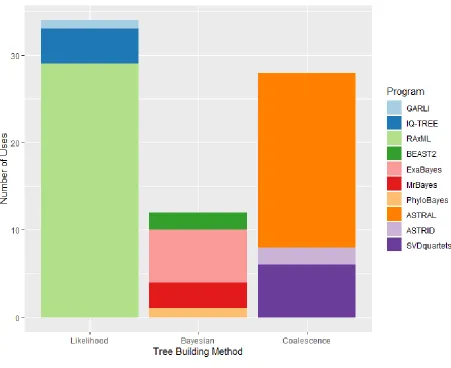
Tree Building 373
Once datasets have been generated, downstream analyses on UCE data are similar to
374
phylogenetic analyses performed on most other data types (e.g. Sanger sequencing, SNPs, etc.).
375
A variety of tree-building methods (Figure 3) can be used for reconstructing phylogeny from
376
UCE datasets, including Maximum Likelihood (ML), Bayesian Inference (BI), or Multispecies
377
Coalescent/Species Tree (MSC). While the intricacies of phylogenetic analyses are beyond the
378
scope of this paper, excellent and detailed overviews – both theoretical and practical – are
379
available (Yang and Rannala 2012, Liu et al. 2015, Bromham et al. 2018, Bravo et al. 2019).
380
18
Maximum likelihood (ML) is a statistical methodology for estimating unknown
382
parameters in a model. ML is widely used in phylogenetic studies due to its use of complex
383
substitution models and its robustness to many violations to the assumptions of these models
384
(Yang and Rannala 2012). The most widely used programs for phylogenetic reconstruction in the
385
ML framework includes RAxML (Stamatakis 2006, Kozlov et al. 2018) and IQ-TREE (Nguyen
386
et al. 2014). One advantage of these programs is their speed, with the former being the dominant
387
method within UCE literature despite having very limited evolutionary model choices. IQ-TREE
388
has gained momentum in recent years for its ability to produce accurate trees without sacrificing
389
speed (Zhou et al. 2018). It includes functions such as ModelFinder for finding appropriate
390
evolutionary models (Kalyaanamoorthy et al. 2017); approximation-based methods such as
391
ultrafast bootstrap (UFBoot) and Shimodaira-Hasegawa like approximate likelihood ratio test
392
(SH-aLRT), which greatly decreases computational time compared to traditional nonparametric
393
bootstrap methods (Guindon et al. 2010, Hoang et al. 2017); and gene/site concordance factors as
394
alternative support measures to illustrate disagreement among loci and sites (Minh et al. 2018).
395
Bayesian Inference and Divergence Dating 396
Like ML, Bayesian inference (BI) is also a general methodology of statistical inference
397
that has been widely adopted for phylogenetic analyses. Bayesian inference differs from ML in
398
that parameters in the models are considered to be random variables within statistical
399
distributions rather than unknown fixed constants (Yang and Rannala 2012). Today BI using the
400
Markov chain Monte Carlo (MCMC) sampling is a widely adopted method used for
401
phylogenetic analysis, as the incorporation of prior knowledge into the analysis offers an
402
appealing alternative to ML even at the cost of slower computational speed (Nascimento et al.
403
2017). The commonly used Bayesian programs for phylogenomics data include BEAST
19
(Drummond and Rambaut 2007), BEAST 2 (Bouckaert et al. 2014), and ExaBayes (Aberer et al.
405
2014). Bayesian analyses are extremely sensitive to prior probabilities set by users, and often
406
default priors may not be appropriate for the data being analyzed as they can affect resulting
407
topologies (Nascimento et al. 2017). Because setting priors can be daunting for beginners, we
408
advise users to resist the all-too-common tendency to employ default settings and instead urge
409
users to follow steps outlined in Bromham et al. (2018) to make informed choices when setting
410
up Bayesian analyses. Running an ‘empty’ analysis without data to allow MCMC algorithm
411
sampling from the prior is a good way of checking whether the data were informative enough to
412
return posterior distributions different from the marginal priors, and to assess for good
413
convergence and mixing of the MCMC chains (Nascimento et al. 2017, Blaimer et al. 2018b).
414
Divergence time estimation analyses can also be implemented for UCE phylogenies to
415
generate dated chronograms, using carefully selected fossils as calibration points. The commonly
416
used node-dating approach assigns the oldest fossil that can be confidently identified to the
417
youngest internal node, imposing the age of the fossil a minimum age constraint (Arcila et al.
418
2015). An alternative method called total-evidence, or tip-dating methods can include all
419
available paleontological information, ameliorating fossil-placement uncertainty while
420
simultaneously incorporating fossil ages into the analysis (Ronquist et al. 2012a). Both of these
421
methods can be implemented for divergence date estimation using Bayesian inference programs
422
such as MrBayes (Ronquist et al. 2012b), BEAST/BEAST2, and the MCMCTree package in
423
PAML (Yang 2007). While MCMCTree is faster computationally, the setup for prior
424
distributions on fossil calibrations is less intuitive. BEAST/BEAST2, by comparison, is easier to
425
understand and offers more analytical options such as the incorporation of fossils directly into
426
the phylogeny with the newly developed node-dating method using the fossilized birth-death
20
model (Heath et al. 2014). The fossilized birth-death model offers an advantage over other
428
methods by combining morphological and molecular data as well as stratigraphic range data
429
from the fossil record, and can be implemented directly in RevBayes (Höhna et al. 2016), or in
430
BEAST2 with add on package sampled-ancestor (Gavryushkina et al. 2014). In general, large
431
data volumes associated with UCEs makes most Bayesian analyses too computationally
432
intensive to be practical. To overcome this limitation, many studies reduce data size by removing
433
taxa or loci in order to reduce the analysis time (Blaimer et al. 2018b, Borowiec 2019). It is also
434
worth noting that tip-dating models have been shown to recover older ages than traditional
node-435
dating models, and might produce inaccurate date estimations (Arcila et al. 2015). Regardless of
436
the approach, the resulting dated chronogram can be then used as input for additional analyses
437
such as ancestral state reconstruction, historical biogeographic analysis, or diversification rates
438
estimation.
439
Multispecies Coalescent/Species Tree 440
One key advance in molecular phylogenetics has been the acknowledgement that high
441
levels of incomplete lineage sorting (ILS) or other stochastic errors can yield misleading results
442
for traditional methods concatenation methods (Liu et al. 2015, Bravo et al. 2019). Incorporation
443
of discordance between gene trees and species trees as a result of high incomplete lineage sorting
444
(ILS), under the MSC model (Heled and Drummond 2009) can alleviate this problem.
445
Commonly used MSC tree summary-based methods such as ASTRAL (Mirarab et al. 2014,
446
Mirarab and Warnow 2015, Zhang et al. 2018) and MP-EST (Liu et al. 2010) are performed in
447
two steps, wherein gene trees are estimated first and separately, then used as input to generate a
448
species tree based on various summaries of coalescent process (Bravo et al. 2019). Because the
449
accuracy of the individual input gene trees directly affects the resulting species tree, these
21
summary-based methods are especially suspectable to gene tree estimation errors (Molloy and
451
Warnow 2018). Therefore, checking individual gene trees for incongruences is advised to ensure
452
species tree accuracy in summary-based methods. Methods such as concordance factors (Ané et
453
al. 2006, Minh et al. 2018) should be used to provide insight into the influence of ILS versus
454
other factors such as introgression on the resulting topology. Alternatively, site-based coalescent
455
method such as SVDquartets (Chifman and Kubatko 2014) and SVDquest (Vachaspati and
456
Warnow 2018) bypass gene tree estimation, and is comparable or even more accurate than
457
summary methods in cases of high ILS (Chou et al. 2015, Molloy and Warnow 2018). Finally,
458
the newly developed StarBEAST2 (Ogilvie et al. 2017) package for BEAST2 is a promising
459
implementation of the full MSC model which can jointly infer gene trees and species trees, but
460
the current version is too computationally intensive to use on large UCE datasets.
461
462
Resources and Costs 463
Most steps of the wet lab protocol can be performed in standard molecular labs that have
464
access to equipment such as a centrifuge and thermocycler. More specialized equipment such as
465
a sonicator for shearing DNA, TapeStation/Bioanalyzer for quantifying DNA, and
466
BluePippin/PippinHT for size selection can all be substituted with cheaper, albeit less accurate
467
alternatives such as restriction enzymes, gel electrophoresis, and magnetic beads.
468
Illumina platforms (HiSeq, NextSeq, NovaSeq) are generally used for UCE studies due to
469
their high throughput and low cost per base pair. The current estimated cost per specimen is
470
approximately $30 – 40 USD, accounting for costs of all reagents in library preparation and
471
paired-end Illumina run (See Supp Table 1 for sample cost breakdown). Some commercial
22
laboratories (e.g. RAPiD Genomics, Gainesville, FL, USA) also offer UCE enrichment services,
473
handling all library preparation, enrichment, and sequencing; customers simply submit DNA
474
extracts and then receive sequence data. Costs associated with such ‘concierge service’ are
475
considerably higher (approximately ~$120 per specimen), but this may be an attractive option for
476
researchers lacking the infrastructure or personnel to undertake wet lab protocols.
477
Having access to high performance computing (HPC) greatly expedites bioinformatic and
478
phylogenomic analyses, especially when processing large batches of samples. While PHYLUCE
479
and many associated data-processing programs can be run in local Linux/Unix environment, the
480
parallelization using HPC will reduce execution time in computationally intensive steps such as
481
demultiplexing and assembly. Similarly, many phylogenomics programs discussed above can
482
also be expedited through this process.
483
484
Data Availability Recommendations 485
One hallmark feature of UCE data is its open source nature, probe sets, protocols, and
486
previously published data are made publicly available, ensuring repeatability – the foundation of
487
open scientific research. To this end, untrimmed raw Illumina reads should be uploaded to public
488
database such as Sequence Read Archive (SRA) once studies are published, giving interested
489
readers the full ability to download and process the data using different trimming settings. All
490
analytical methods such as software and code used to process data should also be made publicly
491
available on repositories such as Dryad or GitHub. UCE contigs can be uploaded to GenBank as
492
targeted locus studies, making the data available for BLAST. The voucher specimens from
493
which DNA was extracted should be deposited in recognized scientific collections and museums;
23
associated information such as collection locality, identification, etc., should be included as
495
metadata with all molecular sequence (Bravo et al. 2019).
496
497
Current and Future Challenges
498
UCE and similar methods offer the ability to generate massive amounts of data from
499
many loci, and yet, despite the increase in data volume, the same concerns that have long
500
plagued phylogenetic analyses remain as relevant as ever: taxon sampling, choice of alignment
501
methods, and composition bias (Bossert et al. 2017, Mclean et al. 2018). Recent research also
502
suggests phylogenomic results can be strongly affected by a tiny proportion of highly biased loci
503
or sites (Shen et al. 2017), and reduction of phylogenetic noise resulting from compositional
504
heterogeneity and saturation can increase congruence among different analytic methods
505
(Borowiec 2019). With that in mind, we strongly encourage performing sensitivity analyses to
506
test the robustness of results when interpreting phylogenomic data (Borowiec 2019, Camacho et
507
al. 2019). As these large datasets are less prone to uncertainty, and instead may give strongly
508
supported wrong results if model violations are not carefully evaluated (Borowiec et al. 2019).
509
The fact that the function of UCEs remains largely unknown is the basis of active
510
research and a current challenge for identifying and modeling UCEs in a phylogenomic context
511
(Bejerano et al. 2004). Vertebrate UCEs are characterized as predominantly non-coding
512
sequences, non-randomly distributed across chromosomes and acting as regulators and/or
513
enhancers of gene expression (Baira et al. 2008, Polychronopoulos et al. 2017). By contrast,
514
studies of invertebrate UCEs reveal that most flanking regions captured include exons
515
(Branstetter et al. 2017a), with the most widely shared loci being either exclusively conserved
24
exons or partially exonic regions in Hymenoptera and Arachnida (Bossert and Danforth 2018,
517
Hedin et al. 2019). This is an exciting discovery, as the exonic flanking regions captured by the
518
UCE process and transcriptome sequence data within these groups can be meaningfully
519
combined, without the need to design specific probe sets to target them, as demonstrated in
520
Apidae (Bossert et al. 2019). However, since the genomic landscapes of different animal taxa
521
can differ substantially, the wider application of combining transcriptomic data with UCEs in
522
other taxonomic groups still needs to be tested. Currently, it appears that the function of UCEs is
523
highly variable, with flanking regions containing exons and introns; whether this variability will
524
affect downstream analyses remains to be seen.
525
Continued refinement of existing probe sets is needed to increase capture success while
526
minimizing duplicates and paralogous loci. It has been shown in the arachnid probe set, different
527
UCE probes sometimes target regions of the same protein, or include non-orthologous sequences
528
(Hedin et al. 2019). This is unsurprising given the wide phylogenetic depth of the probe set,
529
which was designed to target all arachnids, but given that PHYLUCE cannot detect these
non-530
orthologous sequences as the program only removes different contigs hit by probes targeting the
531
same loci (Faircloth 2015), additional manual filtering is needed to ensure the exclusion of
532
misleading paralogous sequences into the final data matrix (Hedin et al. 2019).
533
534
Conclusion
535
Ultraconserved elements-based phylogenomic studies have been rapidly adopted by
536
researchers working on arthropod taxa since their introduction by Faircloth et al. (2012). This
537
review described the versatility of UCE data at both deep and shallow evolutionary scale, and
25
provided a step-by-step guide to generating and analyzing UCEs; we then summarized current
539
practices, challenges, and unresolved questions that surround this active field. Our hope is to
540
make UCE-based phylogenomic studies more accessible to users with diverse taxonomic
541
interests, and thereby deepen our collective understanding of the roles and functions of UCEs
542
across widely divergent taxa. As our understanding of UCEs develops through studies of
543
different organisms, identifying individual genes and incorporation of functional genomics will
544
yield interesting comparative studies across deeply divergent taxonomic groups and provide new
545
insights in the continued pursuit of building the tree of life.
546
547
548
Acknowledgements
549
We would like to thank Michael Branstetter and two anonymous reviewers for comments
550
that greatly improved the manuscript, Eliana Buenaventura, Chris Cohen, Shahan Derkarabetian,
551
Grey Gustafson, Katherine Noble, and Matthew van Dam for informative discussions on UCE
552
research in their perspective groups. We thank Rachel Atchison and Suzy Rodriguez for graphic
553
design assistance.
554
555
References
556
Aberer, A. J., K. Kobert, and A. Stamatakis. 2014. ExaBayes: massively parallel Bayesian
557
tree inference for the whole-genome era. Molecular Biology and Evolution 31: 2553-2556.
558
Alda, F., V. A. Tagliacollo, M. J. Bernt, B. T. Waltz, W. B. Ludt, B. C. Faircloth, M. E. 559
Alfaro, J. S. Albert, and P. Chakrabarty. 2018. Resolving deep nodes in an ancient radiation
26
of neotropical fishes in the presence of conflicting signals from incomplete lineage sorting.
561
Systematic Biology 68: 573-593.
562
Ali, O. A., S. M. O’Rourke, S. J. Amish, M. H. Meek, G. Luikart, C. Jeffres, and M. R. 563
Miller. 2016. RAD Capture (Rapture): Flexible and efficient sequence-based genotyping.
564
Genetics 202: 389-400.
565
Allio, R., A. Schomaker-Bastos, J. Romiguier, F. Prosdocimi, B. Nabholz, and F. Delsuc. 566
2019. MitoFinder: efficient automated large-scale extraction of mitogenomic data in target
567
enrichment phylogenomics. bioRxiv 685412.
568
Andermann, T., A. Cano, A. Zizka, C. Bacon, and A. Antonelli. 2018. SECAPR-a
569
bioinformatics pipeline for the rapid and user-friendly processing of targeted enriched Illumina
570
sequences, from raw reads to alignments. PeerJ 6: e5175.
571
Andermann, T., A. M. Fernandes, U. Olsson, M. Topel, B. Pfeil, B. Oxelman, A. Aleixo, B. 572
C. Faircloth, and A. Antonelli. 2019. Allele phasing greatly improves the phylogenetic utility
573
of ultraconserved elements. Systematic Biology 68: 32-46.
574
Ané, C., B. Larget, D. A. Baum, S. D. Smith, and A. Rokas. 2006. Bayesian Estimation of
575
Concordance among Gene Trees. Molecular Biology and Evolution 24: 412-426.
576
Arcila, D., R. Alexander Pyron, J. C. Tyler, G. Orti, and R. R. Betancur. 2015. An
577
evaluation of fossil tip-dating versus node-age calibrations in tetraodontiform fishes (Teleostei:
578
Percomorphaceae). Molecular Phylogenetics and Evolution 82 Pt A: 131-145.
579
Baca, S. M., E. F. A. Toussaint, K. B. Miller, and A. E. Z. Short. 2017a. Molecular
580
phylogeny of the aquatic beetle family Noteridae (Coleoptera: Adephaga) with an emphasis on
581
data partitioning strategies. Molecular Phylogenetics and Evolution 107: 282-292.
582
Baca, S. M., A. Alexander, G. T. Gustafson, and A. E. Z. Short. 2017b. Ultraconserved
583
elements show utility in phylogenetic inference of Adephaga (Coleoptera) and suggest paraphyly
584
of ‘Hydradephaga’. Systematic Entomology 42: 786-795.
585
Baira, E., J. Greshock, G. Coukos, and L. Zhang. 2008. Ultraconserved elements: genomics,
586
function and disease. RNA Biology 5: 132-134.
587
Baird, N. A., P. D. Etter, T. S. Atwood, M. C. Currey, A. L. Shiver, Z. A. Lewis, E. U. 588
Selker, W. A. Cresko, and E. A. Johnson. 2008. Rapid SNP discovery and genetic mapping
589
using sequenced RAD markers. PLoS One 3: e3376.
590
Bankevich, A., S. Nurk, D. Antipov, A. A. Gurevich, M. Dvorkin, A. S. Kulikov, V. M. 591
Lesin, S. I. Nikolenko, S. Pham, and A. D. Prjibelski. 2012. SPAdes: a new genome assembly
592
algorithm and its applications to single-cell sequencing. Journal of Computational Biology 19:
593
455-477.
594
Bejerano, G., M. Pheasant, I. Makunin, S. Stephen, W. J. Kent, J. S. Mattick, and D. 595
Haussler. 2004. Ultraconserved elements in the human genome. Science 304: 1321-1325.
596
Bi, K., D. Vanderpool, S. Singhal, T. Linderoth, C. Moritz, and J. M. Good. 2012. 597
Transcriptome-based exon capture enables highly cost-effective comparative genomic data
598
collection at moderate evolutionary scales. BMC Genomics 13: 403.
599
Blaimer, B. B., J. R. Mawdsley, and S. G. Brady. 2018a. Multiple origins of sexual
600
dichromatism and aposematism within large carpenter bees. Evolution 72: 1874-1889.
601
Blaimer, B. B., M. W. Lloyd, W. X. Guillory, and S. G. Brady. 2016a. Sequence capture and
602
phylogenetic utility of genomic ultraconserved elements obtained from pinned insect specimens.
603
PLoS One 11: e0161531.
27 Blaimer, B. B., J. S. LaPolla, M. G. Branstetter, M. W. Lloyd, and S. G. Brady. 2016b. 605
Phylogenomics, biogeography and diversification of obligate mealybug-tending ants in the genus
606
Acropyga. Molecular Phylogenetics and Evolution 102: 20-29.
607
Blaimer, B. B., P. S. Ward, T. R. Schultz, B. L. Fisher, and S. G. Brady. 2018b. 608
Paleotropical diversification dominates the evolution of the hyperdiverse ant tribe
609
Crematogastrini (Hymenoptera: Formicidae). Insect Systematics and Diversity 2: 3.
610
Blaimer, B. B., S. G. Brady, T. R. Schultz, M. W. Lloyd, B. L. Fisher, and P. S. Ward. 2015. 611
Phylogenomic methods outperform traditional multi-locus approaches in resolving deep
612
evolutionary history: a case study of formicine ants. BMC Evolutionary Biology 15: 271.
613
Bodily, P. M., M. S. Fujimoto, C. Ortega, N. Okuda, J. C. Price, M. J. Clement, and Q. 614
Snell. 2015. Heterozygous genome assembly via binary classification of homologous sequence.
615
BMC Bioinformatics 16: S5.
616
Bolger, A. M., M. Lohse, and B. Usadel. 2014. Trimmomatic: a flexible trimmer for Illumina
617
sequence data. Bioinformatics 30: 2114-2120.
618
Borowiec, M. L. 2019. Convergent evolution of the army ant syndrome and congruence in
big-619
data phylogenetics. Systematic Biology 68: 642–656.
620
Borowiec, M. L., C. Rabeling, S. G. Brady, B. L. Fisher, T. R. Schultz, and P. S. Ward. 621
2019. Compositional heterogeneity and outgroup choice influence the internal phylogeny of the
622
ants. Molecular Phylogenetics and Evolution 134: 111-121.
623
Bossert, S., and B. N. Danforth. 2018. On the universality of target-enrichment baits for
624
phylogenomic research. Methods in Ecology and Evolution 9: 1453-1460.
625
Bossert, S., E. A. Murray, B. B. Blaimer, and B. N. Danforth. 2017. The impact of GC bias
626
on phylogenetic accuracy using targeted enrichment phylogenomic data. Molecular
627
Phylogenetics and Evolution 111: 149-157.
628
Bossert, S., E. A. Murray, E. A. B. Almeida, S. G. Brady, B. B. Blaimer, and B. N. 629
Danforth. 2019. Combining transcriptomes and ultraconserved elements to illuminate the
630
phylogeny of Apidae. Molecular Phylogenetics and Evolution 130: 121-131.
631
Bouckaert, R., J. Heled, D. Kühnert, T. Vaughan, C.-H. Wu, D. Xie, M. A. Suchard, A. 632
Rambaut, and A. J. Drummond. 2014. BEAST 2: a software platform for Bayesian
633
evolutionary analysis. PLoS Computational Biology 10: e1003537.
634
Branstetter, M. G., and J. T. Longino. 2019. Ultra-conserved element phylogenomics of New
635
World Ponera (Hymenoptera: Formicidae) illuminates the origin and phylogeographic history of
636
the Endemic Exotic Ant Ponera exotica. Insect Systematics and Diversity 3: 1.
637
Branstetter, M. G., J. T. Longino, P. S. Ward, B. C. Faircloth, and S. Price. 2017a. 638
Enriching the ant tree of life: enhanced UCE bait set for genome-scale phylogenetics of ants and
639
other Hymenoptera. Methods in Ecology and Evolution 8: 768-776.
640
Branstetter, M. G., A. Jesovnik, J. Sosa-Calvo, M. W. Lloyd, B. C. Faircloth, S. G. Brady, 641
and T. R. Schultz. 2017b. Dry habitats were crucibles of domestication in the evolution of
642
agriculture in ants. Proceedings of the Royal Society of London B: Biological Sciences 284.
643
Branstetter, M. G., B. N. Danforth, J. P. Pitts, B. C. Faircloth, P. S. Ward, M. L. 644
Buffington, M. W. Gates, R. R. Kula, and S. G. Brady. 2017c. Phylogenomic Insights into the
645
Evolution of Stinging Wasps and the Origins of Ants and Bees. Current Biology 27: 1019-1025.
646
Bravo, G. A., A. Antonelli, C. D. Bacon, K. Bartoszek, M. P. K. Blom, S. Huynh, G. Jones, 647
L. L. Knowles, S. Lamichhaney, T. Marcussen, H. Morlon, L. K. Nakhleh, B. Oxelman, B. 648
28 V. Edwards. 2019. Embracing heterogeneity: coalescing the Tree of Life and the future of
650
phylogenomics. PeerJ 7: e6399.
651
Bromham, L., S. Duchene, X. Hua, A. M. Ritchie, D. A. Duchene, and S. Y. W. Ho. 2018. 652
Bayesian molecular dating: opening up the black box. Biological Reviews 93: 1165-1191.
653
Camacho, G. P., M. R. Pie, R. M. Feitosa, and M. S. Barbeitos. 2019. Exploring gene tree
654
incongruence at the origin of ants and bees (Hymenoptera). Zoologica Scripta 48: 215-225.
655
Capella-Gutiérrez, S., J. M. Silla-Martínez, and T. Gabaldón. 2009. trimAl: a tool for
656
automated alignment trimming in large-scale phylogenetic analyses. Bioinformatics 25:
1972-657
1973.
658
Castresana, J. 2000. Selection of conserved blocks from multiple alignments for their use in
659
phylogenetic analysis. Molecular Biology and Evolution 17: 540-552.
660
Chifman, J., and L. Kubatko. 2014. Quartet inference from SNP data under the coalescent
661
model. Bioinformatics 30: 3317-3324.
662
Chou, J., A. Gupta, S. Yaduvanshi, R. Davidson, M. Nute, S. Mirarab, and T. Warnow. 663
2015. A comparative study of SVDquartets and other coalescent-based species tree estimation
664
methods. BMC Genomics 16: S2.
665
Cooke, C. 2018. Forest Micro-Hymenoptera, including those attacking trees (Cynipidae: Oak
666
Gall Wasps) and those potentially defending them (Parasitic Pteromalidae). PhD, University of
667
Maryland, College Park, MD, USA.
668
Crawford, N. G., B. C. Faircloth, J. E. McCormack, R. T. Brumfield, K. Winker, and T. C. 669
Glenn. 2012. More than 1000 ultraconserved elements provide evidence that turtles are the sister
670
group of archosaurs. Biology Letters rsbl20120331.
671
Cruaud, A., G. Groussier, G. Genson, L. Saune, A. Polaszek, and J. Y. Rasplus. 2018. 672
Pushing the limits of whole genome amplification: successful sequencing of RADseq library
673
from a single microhymenopteran (Chalcidoidea, Trichogramma). PeerJ 6: e5640.
674
Cruaud, A., S. Nidelet, P. Arnal, A. Weber, L. Fusu, A. Gumovsky, J. Huber, A. Polaszek, 675
and J. Y. Rasplus. 2019. Optimized DNA extraction and library preparation for minute
676
arthropods: Application to target enrichment in chalcid wasps used for biocontrol. Molecular
677
Ecology Resources.
678
de Vienne, D. M., S. Ollier, and G. Aguileta. 2012. Phylo-MCOA: a fast and efficient method
679
to detect outlier genes and species in phylogenomics using multiple co-inertia analysis.
680
Molecular Biology and Evolution 29: 1587-1598.
681
Derkarabetian, S., S. Castillo, P. K. Koo, S. Ovchinnikov, and M. Hedin. 2019. A
682
demonstration of unsupervised machine learning in species delimitation. Molecular
683
Phylogenetics and Evolution 139.
684
Derkarabetian, S., J. Starrett, N. Tsurusaki, D. Ubick, S. Castillo, and M. Hedin. 2018. A
685
stable phylogenomic classification of Travunioidea (Arachnida, Opiliones, Laniatores) based on
686
sequence capture of ultraconserved elements. ZooKeys 1-36.
687
Drummond, A. J., and A. Rambaut. 2007. BEAST: Bayesian evolutionary analysis by
688
sampling trees. BMC Evolutionary Biology 7: 214.
689
Edgar, R. C. 2004. MUSCLE: multiple sequence alignment with high accuracy and high
690
throughput. Nucleic Acids Research 32: 1792-1797.
691
Faircloth, B. 2013. Illumiprocessor: a trimmomatic wrapper for parallel adapter and quality
692
trimming.
693
Faircloth, B. C. 2015. PHYLUCE is a software package for the analysis of conserved genomic
694
loci. Bioinformatics 32: 786-788.
29 Faircloth, B. C. 2017. Identifying conserved genomic elements and designing universal bait sets
696
to enrich them. Methods in Ecology and Evolution 8: 1103-1112.
697
Faircloth, B. C., L. Sorenson, F. Santini, and M. E. Alfaro. 2013. A phylogenomic
698
perspective on the radiation of ray-finned fishes based upon targeted sequencing of
699
ultraconserved elements (UCEs). PLoS One 8: e65923.
700
Faircloth, B. C., M. G. Branstetter, N. D. White, and S. G. Brady. 2015. Target enrichment
701
of ultraconserved elements from arthropods provides a genomic perspective on relationships
702
among Hymenoptera. Molecular Ecology Resources 15: 489-501.
703
Faircloth, B. C., J. E. McCormack, N. G. Crawford, M. G. Harvey, R. T. Brumfield, and T. 704
C. Glenn. 2012. Ultraconserved elements anchor thousands of genetic markers spanning
705
multiple evolutionary timescales. Systematic Biology 61: 717-726.
706
Forthman, M., C. W. Miller, and R. T. Kimball. 2019. Phylogenomic analysis suggests
707
Coreidae and Alydidae (Hemiptera: Heteroptera) are not monophyletic. Zoologica Scripta 48:
708
520-534.
709
Frandsen, P. B., B. Calcott, C. Mayer, and R. Lanfear. 2015. Automatic selection of
710
partitioning schemes for phylogenetic analyses using iterative k-means clustering of site rates.
711
BMC Evolutionary Biology 15: 13.
712
Gavryushkina, A., D. Welch, T. Stadler, and A. J. Drummond. 2014. Bayesian inference of
713
sampled ancestor trees for epidemiology and fossil calibration. PLoS Computational Biology 10:
714
e1003919.
715
Gnirke, A., A. Melnikov, J. Maguire, P. Rogov, E. M. LeProust, W. Brockman, T. Fennell, 716
G. Giannoukos, S. Fisher, and C. Russ. 2009. Solution hybrid selection with ultra-long
717
oligonucleotides for massively parallel targeted sequencing. Nature Biotechnology 27: 182.
718
Grab, H., M. G. Branstetter, N. Amon, K. R. Urban-Mead, M. G. Park, J. Gibbs, E. J. 719
Blitzer, K. Poveda, G. Loeb, and B. N. Danforth. 2019. Agriculturally dominated landscapes
720
reduce bee phylogenetic diversity and pollination services. Science 363: 282-284.
721
Grabherr, M. G., B. J. Haas, M. Yassour, J. Z. Levin, D. A. Thompson, I. Amit, X. 722
Adiconis, L. Fan, R. Raychowdhury, and Q. Zeng. 2011. Full-length transcriptome assembly
723
from RNA-Seq data without a reference genome. Nature Biotechnology 29: 644.
724
Guindon, S., J.-F. Dufayard, V. Lefort, M. Anisimova, W. Hordijk, and O. Gascuel. 2010. 725
New algorithms and methods to estimate maximum-likelihood phylogenies: assessing the
726
performance of PhyML 3.0. Systematic Biology 59: 307-321.
727
Gustafson, G. T., A. Alexander, J. S. Sproul, J. M. Pflug, D. R. Maddison, and A. E. Z. 728
Short. 2019. Ultraconserved element (UCE) probe set design: Base genome and initial design
729
parameters critical for optimization. Ecology and Evolution 9: 6933-6948.
730
Harvey, M. G., B. T. Smith, T. C. Glenn, B. C. Faircloth, and R. T. Brumfield. 2016. 731
Sequence capture versus restriction site associated DNA sequencing for shallow systematics.
732
Systematic Biology 65: 910-924.
733
Heath, T. A., J. P. Huelsenbeck, and T. Stadler. 2014. The fossilized birth-death process for
734
coherent calibration of divergence-time estimates. Proceedings of the National Academy of
735
Sciences of the United States of America 111: E2957-2966.
736
Hedin, M., S. Derkarabetian, J. Blair, and P. Paquin. 2018a. Sequence capture
737
phylogenomics of eyeless Cicurina spiders from Texas caves, with emphasis on US
federally-738
endangered species from Bexar County (Araneae, Hahniidae). ZooKeys 49-76.