The transmission effects of the subprime crisis to emerging markets: A global VAR analysis

427

The transmission effects of the subprime crisis to emerging markets

:

A global VAR

analysis

Olfa Manai Daboussi

Laboratory Centre for Macroeconomics, Conjuncture and Method Applied (MACMA)-Higher Institute of Management of Tunis, University of Tunis, Tunisia

Amira Majoul

Applied Quantitative Analysis Unit (UAQUAP)-Tunisia ISG and GATE (UMR 5824 CNRS), Higher Institute of Management of Tunis, University of Tunis, Tunisia

Abstract

The objective of this paper is to analyze the transmission cycle in the United States in emerging markets. In this work we present a quarterly global model (GVAR) that combines individual economies vector error-correcting models in which the domestic variables are related to the country-specific foreign variables. The global VAR (GVAR) model is estimated for 32 countries over the period 1980-2013. It has the advantage of studying the effect of shocks from the U.S to emerging markets in particular the interdependence between national and international cycles. In addition to generalized impulse responses, the current paper considers the use of the GVAR for structural impulse response analysis with focus on external shocks for the emerging economy, particularly in response to shocks to the U.S The results confirm that the U.S plays an important role in the transmission of business cycles and an economic recession affecting the U.S tends to affect emerging economies.

Keywords: Subprime crisis, GVAR, generalized impulse responses, emerging markets

Introduction

The process of globalization has been particularly significant acceleration in emerging from the 90s (Loots, 2002). An expected effect was observed an increase in the degree of synchronization of the cycle in these countries with the rest of the world (mainly the major developed countries).

Emerging countries would thus become sandstone globalization more vulnerable to the volatility of the international economy. However, as shown by the work of Kose et al. (2003), Akin and Kose (2008), Crucini et al. (2008) and Bildirici (2010) far from leading to the formation of a global cycle, globalization seems to have accompanied regional cycles increasingly marked.

The theory of decoupling economic conditions in emerging countries vis-à-vis that of the developed countries is only a manifestation of this result observed before the global financial crisis due to the collapse of the U.S market for subprime mortgages.

Name: Olfa Manai Daboussi Email address:[email protected]

Asian Journal of Empirical Research

428

Various factors have been put forward to explain this evolution. First, many developing countries have experienced rapid development since the 90s. This has contributed, on the one hand, to strengthen their resilience and, secondly, to intensify their mutual relations (through the growth of commercial exchange, called - South-South).

Second, these countries have adopted macroeconomic frameworks with the objectives of stabilizing inflation and control public debt levels.

The objective of this paper is to study the interdependence between the United States and emerging markets. We try to answer the question whether the global economic cycles are converging, or instead whether emerging markets have managed to decouple business cycle fluctuations in the U.S More specifically, we empirically quantify the contemporary impacts of external shocks and to predict future effects of shocks from the U.S to emerging markets.

Thus, we hope to achieve two goals in this work: one is to contribute to the economic literature on the topic; and the other is to have a more reliable yardstick available in order to explore the effects of the subprime crisis to emerging markets by using a Global VAR model during the last period.

The outline of the remainder of the paper is as follows. Section two presents overview of literature. Section three presents the model of the economy and gives the numerical methods used to explore the implications for empirical research. Section four summarizes the main empirical results and finally we present the discussion and conclusion. The paper has additional tables in the appendices.

Review of literature

Several empirical studies have tried to address this problem. These studies are based on simple methods that involve measuring the correlation between these countries and on more sophisticated models using VAR models and factor models.

The first works were based on cross-correlations of the growth rates of activity. Helbling and Bayoumi (2003) find that the correlation coefficients between the United States and the G-7 countries have decrease during the period 1973 to 2001. Similarly, Heathcote and Perri (2004) show that the correlations of output, consumption and investment between the United States and Europe, Canada and Japan are lower during 1986-2000 than in 1972-1985.

Other empirical studies by Frankel and Rose (1998), using panel data confirm the existence of a positive relationship between the intensification of bilateral trade and the correlation of the business cycle, which justifies the role of integration in the synchronization of the business cycle in developed countries. In this regard, Clark and Wincoop (2001), Otto et al. (2001), Calderon et al. (2002), Baxter and Kouparitsas (2004) argue that trade is the main factor that determines the degree of synchronization of the business cycle (see figure 1 and 2 in appendix).

429

growth is influenced by common shocks and in particular by the significant fluctuations in the price of oil.

In other studies the carried out by the IMF (2007), using panel regressions, the SVAR model and the dynamic factors in a sample of 130 developed and developing countries, shows that despite the synchronization between cycles decreased over time, the role of the United States in the transmission cycles of other countries is especially important for neighboring countries. It also shows the importance of regional shocks by comparing the domestic factors and external shocks in volatility cycles. Using the same model Kose et al. (2008) analyzes the evolution of the degree of cyclical inter-dependence; they show the decrease of the influence of common factors to regional factors.

In general, most recent studies based on the dynamic factor model and VAR models to examine the relationships between countries. But the inconvenience of these models is that the former does not allow us to study several transmission channels, while the latter face a problem of identifying factors level.

The model structure and estimations

Patterns for co-movements, for the study of economic cycles between countries, have become more pronounced over the past two decades owing to increased economic and financial integration, with important implications for macroeconomic policy spillovers across countries.

To investigate the mechanisms of transmission of shocks globally, we propose a relatively new approach based on global VAR (GVAR) proposed by Pesaran et al. (2004) and developed by Dees

et al. (2007). The originality of this model is that it takes account of global interdependence in a

transparent manner by integrating a large number of countries. It also takes into account of the international transmission mechanisms channels.

Structural of global VAR (GVAR) framework

In practice, it is assumed that there are N +1 countries (regions) in the global economy, indexed by i = 0, 1, 2…N. « Country 0 » is adopted as the reference country (the United States in this study. For each country (region), it is assumed that the country-specific variables are connected by the global economic variables by VARX*(pi, qi) model as follows:

………. (1)

With xit the vector of variables to model dimension ki × 1; dt vector common to all countries like

for example the international oil price variables; the vector of foreign variables specific to country i of dimension k*

i × 1; Φi (L, pi) and Λi (L, qi)are polynomial matrices of dimensions ki × ki and ki × k *i with the lag (L) and represent the coefficients of the variables in the domestic and foreign countries respectively; ai0 and ai1 are vectors of dimension ki × 1 coefficients of variables

trend. i (L, qi), dimension ki × kd , matrix polynomial coefficients of international variables dt; uit of dimension ki × 1, the vector of idiosyncratic shocks specific to the country. It is assumed that the idiosyncratic shocks uit are uncorrelated with mean 0 and matrix non-singular covariance:

are constructed from weighted Specific foreign country variables

averages of the corresponding relative to other countries variables. They measure the impact of trade partners on the economy in question. These variables are obtained as follows:

* it

x



* it

x

it it i i t i i i i it i

i L p x a a t  L q d  L q x u

 *

1

0 ( , ) ( , )

) ,

(



)

,

0

(

it

iid

430

when . represents the share of country j in the trade (Exports + Imports/ Total of trade) of country i.

After selecting the lag pi and qi in each country by the AIC (assuming 2 as maximum lag), we estimate the models VARX* separately for each country for the possibility of cointegration

between xit , and dt. Once the country-specific models estimated, all endogenous variables in

the global economy are collected together in a vector xt = (x’0t, x’1t, ..., x’N t) with:

that represents the number of variables in the endogenous global model. For this, the model VARX * can be rewritten as follows:

for (i= 0, 1, 2,…, N) ……….. (2)

Where , ,

Let p= max (p0, p1, ..., pN, q0, q1, ..., qN), and construct Ai (L, p) from Ai (L, pi, qi). Also note that:

, i=0, 1,2…, N ………. (3)

With Wi is a (ki + k*i ) × k matrix defined by the country specific weights Wij. With the above notations (2) can be written equivalently as:

i =0,1,…, N,

and then stacked to yield the VAR(p) model in xt: The GVAR is as follows:

... (4)

Specification and estimation of the country-specific models

Dataset

The proposed model takes into account 32 countries, including 28 countries, the US, China, Japan and the UK and 28 countries aggregated into regions covering the period 1980-2013 with quarterly data (see table A in appendix). The GVAR model includes the following variables: the real output2_{, the rate of inflation}3_{, the exchange rate in terms of US dollars}4_{, real equity prices}5_{, the} short interest rates6_{, the long interest rates}7 _{and oil prices.}

it = ln (GDPit/ CPIit) 3 _π

it = pit - pit-1 with pit = ln (CPI it) 4 _{Ln (e}

it)-pit 5 _q

it = Ln (EQit/CPI) 6 _ρS

it = 0.25*ln (1+RSit/100) 7 _ρL

it = 0.25*ln (1+RLit/100)

, 0 *





0







* it

x



( i i i i i i

i L p q L p L q

A    

        * it it it x x z it t i i i i

it a0 a1t (L,q )d u



t i it

W

x

z



,

p

(L,

Ai



W

x





t t

x p L

G( , ) 

it it i i

i

L

p

q

z

431

These data are all collected on the website of the International Monetary Fund and from International Financial Statistics. For countries where GDP is available only annually, we proceeded to the method of interpolation used by Dees et al. (2007), we estimated the GVAR model using the Gauss Program.

Estimation and GVAR model specification

To estimate the country specific models we have carried out preliminary tests such as tests of stationarity (ADF test and test WS) and the exogeneity test (Johansen, 1992 and Harbo et al.,

1998). We noticed that introduced endogenous and exogenous variables are integrated of order 1. The assumption of weak exogeneity is not rejected for most variables confirming the hypothesis of weak exogéinité. Indeed, we found only 7 cases out of 159 cases are significant at the 5% level8_.

As we said the key to our strategy is the weak exogeneity assumption of x*

it. This test involves testing the significance of estimating the error correction term in the auxiliary equation of variables specific of foreign countries, x*

it. In particular, each l th element of x*it the following regression is carried out:

…… (5)

Where ECMj

i,t−1, j = 1, 2, ..., ri are the estimated error correction terms corresponding to the ri cointegrating relations found for the ith _{country model and Δ = (Δx}’*

it, Δ(e*it − p*it), Δp0t)’. The test for weak exogeneity is an F-test of the joint hypothesis that γij, l = 0, j = 1, 2... ri in the above regression. The lag orders si and ni, need not be the same as the orders pi and qi of the underlying country-specific VARX* models. In our case, for this test, we imposed the order of 2 lag on all foreign variables and we assumed that si = pi.

The dynamic analysis of the GVAR model: impulse response functions

One of the important tools in the analysis of dynamical systems is the impulse response function that characterizes the possible reaction of the system to different future periods to the effect of shock variables in the model. To do so we used the general impulse response function developed by Koop et al. (1996) in their non-linear model. It allows studying the dynamics of transmission of shocks. It considers the impact associated with the error of a single variable on the variable lth _of ith _{model using their historical distributions observed. It is defined as follows:}

GIx,εil(n,√σii,ll, It−1) = E (xt+n/εilt=√σii,ll,It−1) − E(xt+n/It−1) ……….(6)

With it-1 shows all available information (t-1) and σii,ll designates the variance of the error

termεii,ll. This function allows studying the dynamics of the global model and estimating the

magnitude of the effects of shocks to foreign variables: negative shock in equity prices in the U.S, a positive shock to oil prices and negative demand shock to U.S. In our study we limit the simulations to 2008.

Empirical results

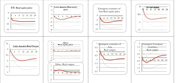
Figure 3 shows the response of macroeconomic variables following a negative shock to stock prices in the United States over a period of two years using the bootstrap technique. This shock is equivalent to a 5% decrease in share price. It is immediately sent to different markets. This

8_{Test results are available on request from the authors}

* , ~ m t i x 







 ri i i

j s k n m l i t m t i t i m k t i l i k j t i l i j i l l

i t ECM x x

x

1 1 1

432

confirms the important role of the market capitalization of the U.S in the global economy and the importance of the financial channel in the transmission of shocks. This effect is more pronounced in India, the region of emerging Asia and Latin America. The shock response of African financial markets is relatively low. This is an expected result if we take into account the low level of international financial integration in the region. Then, a decline in GDP of 0.8% U.S shows the dependence of the actual activity of these regions of U.S external funding. Indeed, sudden stops in these regions are the main cause of the decline in GDP. This can be explained by the withdrawal of foreign investors from their financial investments.

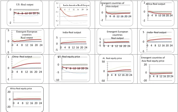
Shock associated with a decline in demand from the U.S (figure 4) show that this shock is equivalent to a decrease of 0.4 % of GDP in the US. This will negatively impact but slowly transmitted to the GDP of Latin America and emerging Asia. For Africa, we have seen a decline in GDP more important than the shock associated with the equity prices. This result suggests that the trade channel between this region and the United States is more important than the financial channel. The decrease in GDP in the U.S will affect demand for raw materials as well as their prices.

China and India are not affected by the shock. This can be explained by the fact that these economies have become more independent of the U.S, boosting intra-regional trade. This idea was confirmed by IMF (2007).

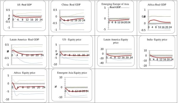
Figure 5 show the oil price shock. The 12 % increase in oil prices has a negative effect on the GDP of the U.S decreases by 0.08 % after one quarter before leveling quickly. The impact on oil prices negatively affects all emerging markets. This suggests that the dependence of these countries on oil is needed to manufacture all kinds of products. In our sample, Saudi Arabia and Mexico are the two largest exporters of oil, they recorded low growth, but the effect wears off quickly. Concerning equity prices, as expected, the reaction will be negative in all regions.

Discussion and conclusion

433

than the trade channel in the transmission of shocks to emerging markets. These countries remain until today heavily dependent on foreign capital flows in the form of foreign direct investment. The effect of real shock decreased since these countries were able to develop intra-regional trade and exploit other markets.

In this respect, our study was not limited to these two types of shocks. In this framework we have integrated our analysis the effect of the common stock through the variable oil prices. It negatively affects all emerging markets. This situation is exacerbated by inflationary pressures showing the dependence of these economies to oil prices.

Finally, our work has shown shortcomings. The choice of macroeconomic variables is limited. In our study, promising new tracks can be addressed in order to further expand the topics discussed in this work. We propose two possible extensions.

The first is to further research on fiscal and monetary policy in emerging markets during the effects of the subprime crisis. We can focus our research by studying the question of the effectiveness of these policies in major emerging markets. This allows us to draw the economic and financial characteristics relating to each emerging countries and compare them. Second is to develop the econometric method. Binder and Gross (2013) develop a Regime-Switching Global Vector Autoregressive (RS-GVAR) model. The RS-GVAR model allows for recurring or non-recurring structural changes in all or a subset of countries. It can be used to generate regime-dependent impulse response functions which are conditional upon a regime-constellation across countries.

References

Akin, C., & Kose, M. A. (2008). Changing nature of north-south linkages: Stylized facts and explanations. Journal of Asian Economics, 19, 1–28.

Altug, S., & Bildirici, M. (2010). Business cycles around the globe: a regime-switching approach.

TÜSİAD-KOÇ university economic research forum, working paper 100.

Baxter, M., & Kouparitsas, M. (2004). Determinants of business cycle comovement: a robust analysis. NBER Working paper number 10725.

Binder, M., & Gross, M. (2013). Regime-switching global vector autoregressive models. European central bank working paper series S, No 1569.

Calderón, C., Chong, A., & Stein, E. (2002). Trade intensity and business cycle synchronization:

are developing countries any different? Central bank of Chile working paper, No.195.

Canova, F. (2003). The transmission of US shocks to Latin America. Economics working papers 925, department of economics and business, Universitat Pompeu Fabra.

Clark, T. E., & Wincoop, E. V. (2001). Borders and business cycles. Journal of International

Economics, 55, 59-85.

Crucini, M. J., Kose, M. A. & Otrok, C. (2008). What are the driving forces of international

business cycles? NBER working papers number 14380.

Dees, S., Mauro, D. F., Pesaran, M., & Smith, L. (2007). Exploring the International Linkages of the euro area: A global VAR analysis. Journal of Applied Econometrics, 22(1), pp 1–38. Frankel, J. A., & Rose, A. K. (1998). The endogenity of the optimum currency area Criteria.

Economic Journal, July, pp 1009-1025.

Harbo, I., Johansen, S., Nielsen, B., & Rahbek, A., (1998). Asymptotic inference on cointegration rank in partiel systems. Journal of Business and Economic Statistics, 16, 388-399.

Heathcote, J., & Perri, F. (2004). Financial globalization and real regionalization. Journal of

434

Helbling, T. & Bayoumi, T. (2003). Are They All in the Same Boat? The 2000-2001 Growth Slowdown and the G-7 Business Cycle Linkages IMF Working Paper 03/46.

Gross, M., & Kok, C. (2013). Amixed-cross-section GVAR for countries and banks. ECB working paper No. 1570.

Johansen, S. (1992). Co integration in partial systems and the efficiency of single equation analysis. Journal of Econometrics, 52, 389–402.

Koop, G., Pesaran, M. H., Potter, S. M. (1996). Impulse response analysis in nonlinear multivariate models. Journal of Econometrics, 74, 119-147.

Kose, M. A., Otrok, C., & Prasad, E. (2008). Global business cycles: convergence or decoupling? IMF working papers 08/143.

Kose, A., Prasad, E., & Terrones, M. (2003). How does globalization affect the synchronization of business cycles? American Economic Review, 93, 57-62.

Loots, E. (2002). Globalisation, emerging markets and the South African economy. The South

African Journal for Economics, 70(2), 263-286.

International Monetary Fund (2007). Spillovers and cycles in the global economy. world economic outlook.

Otto, G., Voss, G., & Willard, L. (2001). Understanding OECD output correlations. Reserve bank of Australia research discussion paper, No. 2001-5.

Pesaran, M. H., Schuermann, T., & Weiner, S. C. (2004). Modeling regional interdependencies using a global error correcting macroeconomic model. Journal of Business and Economic

Statistics, 22, 129-162.

Stock, J. H., & Watson, M. W. (2005). Understanding changes in international business cycles dynamics. Journal of European Economic Association, 3(5), 968-1006.

Appendix

Table A: Countries and regions in the GVAR model

United States European area Latin America

China Japan

United Kingdom

Germany France

Italy Belgium

Finland Netherlands

Argentina Brazil

Chile Mexico

Peru Colombia Developed countries Emerging Asian countries Emerging Europe

Canada New Zealand Norway

Korea Singapore

Thailand Philippines

Indonesia

Poland Turkey

Africa Rest of the world

Tunisia Egypt Morocco South Africa

435

Figure 1: Export to china as a percentage of total exports

Intra-regional exports on % of total exports Export to USA on % of total exports

Figure 2: The share of exports across regions

Source: Autor's calculations based on Direction of Trade Statistics and IMF Source: Autor's calculations based on Coordinated Portfolio Investment Survey and IMF 0

5 10 15 20

1990 1995 2000 2005 2007 2010 2013

Emerging and Developing Asia

Emerging and Developing Countries

Emerging and Developing Europe

Latin America

0 5 10 15 20 25 30 35 40 45

19

90

19

95

20

00

20

05

20

07

20

10

20

13

Emerging and Developing Asia

Emerging and Developing Countries Emerging and Developing Europe Middle East and North Africa Latin America

0 10 20 30 40 50 60 70

19

90

19

95

20

00

20

05

20

07

20

10

20

13

Emerging and Developing Asia

436

Figure 3: Generalized impulse responses of a negative unit shock to U.S. real equity prices (bootstrap mean estimates with 90% bootstrap bounds)

-15 -10 -5 0

0 4 8 12 16 20 24

US-Real equity price

-15 -10 -5 0

0 4 8 12 16 20 24 Emergent countries of

Asia Real equity price

-2 -1 0 1

0 4 8 12 16 20 24 Africa -Real output

-2.5 -2 -1.5 -1 -0.5 0 0.5 1

0 4 8 12 16 20 24 Emergent countries of

Asia Real output

-2 -1.5 -1 -0.5 0 0.5 1 1.5 2

0 4 8 12 16 20 24 Emergent European

437

Figure 4: Generalized impulse responses of a negative shock of the demand in united state (bootstrap mean estimates) -2

0

0 4 8 12 16 20 24 US -Real output

-2 0 2

0 4 8 12 16 20 24

Emergent countries of Asia output

-2 0 2

0 4 8 12 16 20 24

Africa-Real output

-5 0 5

0 4 8 12 16 20 24

Emergent European countries Real output

-5 0 5

0 4 8 12 16 20 24

India-Real output

-5 0 5

0 4 8 12 16 20 24

Emergent European countries Real output

-5 0 5

0 4 8 12 16 20 24

India- Real output

-1 0 1

0 4 8 12 16 20 24

China- Real output

-10 -5 0 5

0 4 8 12 16 20 24

US- Real equity price

-50 0 50

0 4 8 12 16 20 24 AL Real equity price

-20 0 20

0 4 8 12 16 20 24

Emergent countries of Asia Real equity price

-20 0 20

0 4 8 12 16 20 24

438

Figure 5: Generalized impulse responses of a negative shock of oil prices in united state (bootstrap mean estimates) -1

-0.5 0 0.5

0 4 8 12 16 20 24

%

US -Real GDP

-1 -0.5 0 0.5

0 4 8 12 16 20 24 China- Real GDP

-5 0 5

0 4 8 12 16 20 24 Emerging Europe of Asia

Real GDP

-0.5 0 0.5 1

0 4 8 12 16 20 24

%

Africa-Real GDP

-1 -0.5 0 0.5

0 4 8 12 16 20 24

%

Latain America- Real GDP

-10 -5 0 5

0 4 8 12 16 20 24

%

US - Equity price

-40 -20 0 20

0 4 8 12 16 20 24 Latain America Equity

price

-20 -10 0 10

0 4 8 12 16 20 24 India- Equity price

-10 -5 0 5

0 4 8 12 16 20 24

Africa- Equity price

-10 0 10

0 4 8 12 16 20 24

%